


Abstract
We present a new, semi-analytical model describing the evolution of dark matter subhaloes. The model uses merger trees constructed using the method of Parkinson et al. to describe the masses and redshifts of subhaloes at accretion, which are subsequently evolved using a simple model for the orbit-averaged mass-loss rates. The model is extremely fast, treats subhaloes of all orders, accounts for scatter in orbital properties and halo concentrations, uses a simple recipe to convert subhalo mass to maximum circular velocity, and considers subhalo disruption. The model is calibrated to accurately reproduce the average subhalo mass and velocity functions in numerical simulations. We demonstrate that, on average, the mass fraction in subhaloes is tightly correlated with the ‘dynamical age’ of the host halo, defined as the number of halo dynamical times that have elapsed since its formation. Using this relation, we present universal fitting functions for the evolved and unevolved subhalo mass and velocity functions that are valid for a broad range in host halo mass, redshift and Λ cold dark matter cosmology.
1 INTRODUCTION
Numerical N-body simulations have shown that when two dark matter haloes merge, the less massive progenitor halo initially survives as a self-bound entity, called a subhalo, orbiting within the potential well of the more massive progenitor halo. These subhaloes are subjected to tidal forces and impulsive encounters with other subhaloes causing tidal heating and mass stripping, and to dynamical friction that causes them to lose orbital energy and angular momentum to the dark matter particles of the ‘host’ halo. Depending on its orbit, density profile and mass, a subhalo therefore either survives to the present day or is disrupted; the operational distinction being whether a self-bound entity remains or not.
Characterizing the statistics and properties of dark matter subhaloes is of paramount importance for various areas of astrophysics. First of all, subhaloes are believed to host satellite galaxies, and the abundance of satellite galaxies is therefore directly related to that of subhaloes. This basic idea underlies the popular technique of subhalo abundance matching (e.g. Vale & Ostriker 2004; Conroy, Wechsler & Kravtsov 2006, 2007; Guo et al. 2010; Hearin et al. 2013) and has given rise to two problems in our understanding of galaxy formation: the ‘missing satellite’ problem (Klypin et al. 1999a,b; Moore et al. 1999) and the ‘too big to fail’ (TBTF) problem (Boylan-Kolchin, Bullock & Kaplinghat 2011). Secondly, substructure is also important in the field of gravitational lensing, where it can cause time-delays (e.g. Keeton & Moustakas 2009) and flux-ratio anomalies (Metcalf & Madau 2001; Bradač et al. 2002; Dalal & Kochanek 2002), and for the detectability of dark matter annihilation, where the clumpiness due to substructure is responsible for a ‘boost factor’ (e.g. Diemand, Kuhlen & Madau 2007; Giocoli, Pieri & Tormen 2008b; Pieri, Bertone & Branchini 2008). Finally, the abundance and properties of dark matter substructure controls the survivability of fragile structures in dark matter haloes, such as tidal streams and/or galactic discs (Tóth & Ostriker 1992; Taylor & Babul 2001; Ibata et al. 2002; Carlberg 2009).
The most common statistics used to describe the substructure of dark matter haloes are the subhalo mass function (SHMF) and velocity function (SHVF), which express the abundance of subhaloes as function of their mass and maximum circular velocity. In this paper, we distinguish three different mass and velocity functions. The evolved SHMF/SHVF describe the abundance of subhaloes present at any given point in time, t0, as function of their mass and velocity at time t0. The unevolved SHMF/SHVF give the abundance of all subhaloes ever accreted into the main progenitor of the host halo, as function of their mass or velocity at the time of accretion. This includes subhaloes that have been disrupted since their accretion, and are no longer present at time t0. And finally, we consider the unevolved, surviving SHMF/SHVF, which is the same as its unevolved counterpart, but this time only counting the survived subhaloes that are still present at time t0.
SHMFs and SHVFs have been studied using two complementary techniques; N-body simulations (e.g. Tormen 1997; Ghigna et al. 1998, 2000; Moore et al. 1998, 1999; Tormen, Diaferio & Syer 1998; Klypin et al. 1999a,b; Stoehr et al. 2002; De Lucia et al. 2004; Diemand, Moore & Stadel 2004; Gao et al. 2004; Gill, Knebe & Gibson 2004a; Gill et al. 2004b; Kravtsov et al. 2004; Reed et al. 2005; Giocoli, Tormen & van den Bosch 2008a; Weinberg et al. 2008; Giocoli et al. 2010) and semi-analytical techniques based on the extended Press-Schechter (EPS; Bond et al. 1991) formalism (e.g. Taylor & Babul 2001, 2004, 2005a,b; Benson et al. 2002; Taffoni et al. 2003; Zentner & Bullock 2003; Oguri & Lee 2004; Peñarrubia & Benson 2005; van den Bosch, Tormen & Giocoli 2005; Zentner et al. 2005; Gan et al. 2010; Yang et al. 2011; Purcell & Zentner 2012). Both methods have their own pros and cons. Numerical simulations have the virtue of including all relevant, gravitational physics related to the assembly of dark matter haloes, and the evolution of the subhalo population. However, they are also extremely CPU intensive, and the results depend on the mass- and force-resolution adopted. In addition, there is some level of arbitrariness in how to identify haloes and subhaloes in the simulations. In particular, different (sub)halo finders applied to the same simulation output typically yield SHMFs that differ at the 10–20 per cent level (Knebe et al. 2011, 2013; Onions et al. 2012) or more (van den Bosch & Jiang 2016). Semi-analytical techniques, on the other hand, have the advantage that they do not require any subhalo finders, and are significantly faster, but their downsize is that the relevant physics is only treated approximately. In addition, they typically need to be calibrated against numerical simulations results, thereby inheriting all their potential shortcomings.
All semi-analytical methods require two separate ingredients: halo merger trees, which describe the hierarchical assembly of dark matter haloes, and a treatment of the various physical processes that cause the subhalo population to evolve (dynamical friction, tidal heating and stripping, impulsive encounters). To properly account for all these processes, which depend strongly on the orbital properties, requires a detailed integration over all individual subhalo orbits. This is complicated by the fact that the mass of the parent halo evolves with time. If the mass growth rate is sufficiently slow, the evolution may be considered adiabatic, thus allowing the orbits of subhaloes to be integrated analytically despite the non-static nature of the background potential. This principle is exploited in many of the semi-analytical-based models listed above. In reality, however, haloes grow hierarchically through (major) mergers, making the actual orbital evolution non-adiabatic; the merger causes violent relaxation, during which there are no isolating integrals of motion.
In order to sidestep these difficulties, van den Bosch et al. (2005, hereafter B05) considered the average mass-loss rate of dark matter subhaloes, where the average is taken over the entire distribution of orbital configurations (energies, angular momenta and orbital phases). This removes the requirement to actually integrate individual orbits, allowing for an extremely fast generation of large samples of subhaloes. B05 adopted a simple functional form for the average mass-loss rate, which had two free parameters which they calibrated by comparing the resulting SHMFs to those obtained using numerical simulations. In a subsequent paper, Giocoli et al. (2008a, hereafter G08), directly measured the average mass-loss rate of dark matter subhaloes in numerical simulations. They found that the functional form adopted by B05 adequately describes the average mass-loss rates in the simulations, but with best-fitting values for the free parameters that are substantially different. G08 argued that this discrepancy arises from the fact that B05 used the ‘N-branch method with accretion’ of Somerville & Kolatt (1999, hereafter SK99) to construct their halo merger trees, which results in an unevolved SHMF that is significantly different from what is found in the simulations. This was recently confirmed by the authors in a detailed comparison of merger tree algorithms (>Jiang & van den Bosch 2014a, hereafter JB14). Note that the SK99 method has also been used by most of the other semi-analytical models for dark matter substructure, including Taylor & Babul (2004, 2005a,b), Zentner & Bullock (2003), Zentner et al. (2005) and even the recent study by Purcell & Zentner (2012).
An important aspect of subhalo evolution that was overlooked by B05 is the complete destruction of subhaloes due to tidal heating and stripping. Wildly different findings exist regarding, first, whether disruption is physical or due to numerical artefacts, and secondly, the criteria for disruption to happen (e.g. Hayashi et al. 2003; Taylor & Babul 2004; Zentner et al. 2005; Diemand et al. 2007; Gan et al. 2010; Macciò et al. 2010; Wetzel & White 2010). We find that subhalo disruption is ubiquitous in numerical simulations, and thus must be considered in order to reproduce the subhalo populations from simulations.
In this series of papers, we use a significantly upgraded version of the semi-analytical method pioneered by B05 to study the statistics of dark matter subhaloes in unprecedented detail. In particular, we extent and improve B05 by (i) using halo merger trees constructed with the more reliable method of Parkinson, Cole & Helly (2008), (ii) evolving subhaloes using an improved mass-loss model that accounts for stochasticity in the mass-loss rates due to the scatter in orbital properties and halo concentrations, (iii) considering the entire hierarchy of dark matter subhaloes (including sub-subhaloes, sub-sub-subhaloes, etc.), (iv) predicting not only the masses of subhaloes, but also their maximum circular velocities and (v) including a simple treatment of subhalo disruption.
In this paper, the first in the series, we present the improved semi-analytical model, followed by a detailed study of the average subhalo mass and velocity functions. In van den Bosch & Jiang (2016, hereafter Paper II), we present a more detailed comparison of the model predictions with simulation results, paying special attention to the large discrepancies among different simulation results that arise from the use of different subhalo finders. In Paper III (Jiang & van den Bosch in preparation), we exploit our semi-analytical model to quantify the halo-to-halo variance of subhalo populations in unprecedented detail. Finally, in Jiang & van den Bosch (2015) we have applied our model to assess the severity of the ‘TBTF’ problem, by studying the halo-to-halo variance of the subhalo populations of thousands of Milky Way (MW) sized host haloes.
This paper is organized as follows. In Section 2, we describe our semi-analytical model, including the halo merger trees (Section 2.1), the evolution of subhalo mass (Section 2.2) and maximum circular velocity (Section 2.3), the treatment of subhalo disruption (Section 2.4), and how all the ingredients are combined to generate subhalo populations (Section 2.5). In Section 3, we demonstrate that the model can accurately reproduce both the subhalo mass and velocity functions obtained from numerical simulations. In Section 4, we discuss the scaling of the average SHMFs and SHVFs with host halo mass, redshift and cosmological parameters, and present a universal fitting formula applicable to a broad range of host halo mass, redshift and Λ cold dark matter (ΛCDM) cosmology. We summarize our results in Section 5.
2 MODEL DESCRIPTION
The goal of this series of papers is to present a study of unprecedented detail regarding the statistics of dark matter subhaloes. To that extent we use an improved and extended version of the semi-analytical model of B05 which computes the masses of subhaloes for a particular realization of a host halo mass. In what follows we present a detailed description of the model, including a discussion of how and where we make improvements, and add extensions, with respect to the B05 model.
2.1 Halo merger trees
The backbone of the B05 model, and of any other semi-analytical model for the substructure of dark matter haloes, is halo merger trees, which describe the hierarchical mass assembly of dark matter haloes, and therefore give the masses and redshifts at which dark matter subhaloes are accreted on to their hosts.
Before describing the construction of our merger trees, it is useful to introduce some terminology that is used throughout this paper. Fig. 1 shows a schematic representation of a merger tree. We refer to the halo at the base of the tree (i.e. the large purple halo at z = z0) as the host halo. For each individual branching point along the tree, the end product of the merger event is called the descendant halo, while the haloes that merge are called the progenitors. The main progenitor of a descendant halo is the progenitor that contributes the most mass. For example, for the branching point highlighted in Fig. 1, the purple halo at z = z2 is the main progenitor of its descendant at z = z1. The main branch of the merger tree is defined as the branch tracing the main progenitor of the main progenitor of the main progenitor, etc. (i.e. the branch connecting the purple haloes). Note that the main progenitor halo at redshift z is not necessarily the most massive progenitor at that redshift. Throughout we shall occasionally refer to the main progenitors of a host halo as its zeroth-order progenitors, while the mass history, M(z), along this branch is called the mass assembly history (MAH). Haloes that accrete directly on to the main branch are called first-order progenitors, or, after accretion, first-order subhaloes. Similarly, haloes that accrete directly on to first-order progenitors are called second-order progenitors, and they end up at z = z0 as second-order subhaloes (or sub-subhaloes). The same logic is used to define higher order progenitors and subhaloes, as illustrated in Fig. 1. An nth-order (sub)halo that hosts an (n + 1)th-order subhalo is called a parent halo of the (n + 1)th-order subhalo. Throughout, we define (sub)halo masses such that the mass of an nth-order parent halo includes the masses of its subhaloes of order n + 1; we refer to this as the inclusive definition of subhalo mass.
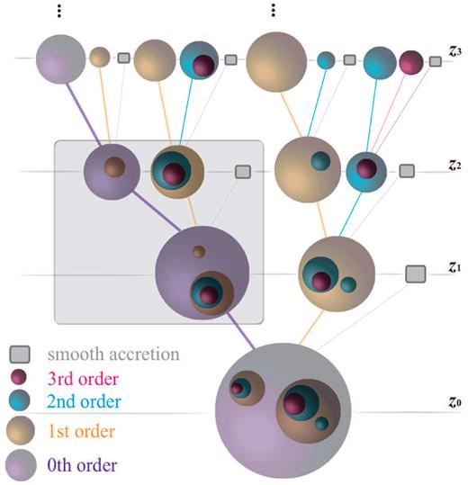
Anatomy of a merger tree for a host halo (purple sphere at the bottom) at redshift z = z0. The purple spheres indicate the assembly history of the main progenitor. We refer to these as ‘zeroth-order’ progenitors, and they accrete ‘first-order’ progenitors (orange), which end up as first-order subhaloes at z = z0. In turn, these first-order progenitors accrete second-order progenitors (blue) which end up as second-order subhaloes (sub-subhaloes) at z = z0, etc. The large, shaded box highlights a single branching point, which is the building block of a merger tree. The small shaded boxes present at each branching point reflect ‘smooth accretion’.
We construct our merger trees using the EPS formalism. EPS provides the progenitor mass function (PMF), nEPS(Mp, z1|M0, z0), describing the ensemble-average number, nEPS(Mp, z1|M0, z0)dMp, of progenitors of mass Mp ± dMp/2 that a descendant halo of mass M0 at redshift z0 has at redshift z1 > z0. Starting from some target host halo mass M0 at z0, one can sample the PMF to draw a set of progenitor masses Mp,1, Mp,2, …, Mp,N at some earlier time z1 = z0 + Δz, where |$\sum _{i=1}^{N} M_{{\rm p},i} = M_0$| in order to assure mass conservation.1 The time step Δz used sets the ‘temporal resolution’ of the merger tree, and may vary along the tree. This procedure is then repeated for each progenitor with mass Mp, i > Mres, thus advancing ‘upwards’ along the tree. The minimum mass, Mres, sets the ‘mass resolution’ of the merger tree and is typically expressed as a fraction of the final host mass M0. The small shaded boxes in Fig. 1, present at each branching, reflect the mass accreted by the descendant halo in the form of smooth accretion (i.e. not part of any halo) or in the form of progenitor haloes with masses Mp < Mres. Throughout we shall refer to this component as smooth accretion.
Haloes at the top of the tree that have no progenitors with mass Mp > Mres are called the leave haloes of the tree, and the mass evolution of a leave halo down to z = 0 is called the halo's trajectory. Only one trajectory per tree corresponds to a host halo (namely that of the main progenitor), while all other trajectories end up as subhaloes at z = 0 (of different orders). The moment a halo is for the first time accreted into a more massive halo (i.e. transits from being a host halo to a subhalo) is called the halo's accretion time, tacc, and its mass at that time is called the accretion mass, macc. Throughout we use the subscript ‘0’ to refer to halo properties at redshift z = z0 (typically we adopt z0 = 0); and we use the subscript ‘acc’ to refer to halo properties at the time of accretion.
B05 constructed EPS merger trees using the SK99 method, but only up to first-order subhaloes, and therefore did not require merger trees that resolve the assembly histories of first-order progenitors. We extend this by using full merger trees, thus allowing us to study the statistics of subhaloes of all orders. In addition, we also improve upon B05 by using another method to construct our merger trees. In JB14, we tested and compared multiple Monte Carlo algorithms for constructing EPS-based merger trees, including SK99. We showed that the SK99-method results in merger rates that are too high by up to a factor of three (see also Fakhouri & Ma 2008; Genel et al. 2009), and thus haloes of given present-day mass that assemble too late. As first pointed out by G08, and as discussed in more detail in JB14, this explains why B05 inferred an average subhalo mass-loss rate that is too high (see Section 2.2). It also implies that other models for dark matter substructure that are based on the SK99 algorithm (Zentner & Bullock 2003; Taylor & Babul 2004,2005; Zentner et al. 2005; Purcell & Zentner 2012), are likely to suffer from similar systematic errors.
Of all the methods tested by JB14, the one that clearly stood out as the most reliable is that of Parkinson et al. (2008, hereafter P08). The P08 algorithm is a modification of the binary algorithm of Cole et al. (2000), in which the PMF is modified with respect to the EPS prediction to match results from the Millennium simulation (see Cole et al. 2008). As shown in JB14, the P08 algorithm yields merger statistics indistinguishable from simulation results. Hence, in this paper we adopt the P08 algorithm. Throughout we always adopt a mass resolution of ψres ≡ Mres/M0 = 10−5 unless stated otherwise, and construct the merger trees using the time stepping advocated in appendix A of P08 (which roughly corresponds to Δz ∼ 10−3; somewhat finer/coarser at high/low redshift). In order to speed up the code, and to reduce memory requirements, we down-sample the time resolution of each merger tree by registering progenitor haloes every time step Δt = 0.1 tff(z). Here tff(z) ∝ (1 + z)−3/2 is the free-fall time for a halo with an overdensity of 200 at redshift z. Since the orbital time of a subhalo is of order the free-fall time, there is little added value in resolving merger trees at higher time resolution than this. We have verified that indeed our results do not change if we use merger trees with a smaller time step.
2.2 Subhalo mass evolution
Although the subhalo mass-loss rate in a static halo is a well-defined concept, in reality the parent mass M increases with time due to the accretion of matter and other subhaloes. Following B05, we utilize the discrete time stepping of the merger tree to evolve both m and M. At the beginning of each time step, the parent halo is assumed to instantaneously increase its mass as described by the merger tree (|$\skew4\dot{M} > 0, \dot{m}=0$|), while in between two time steps we set |$\skew4\dot{M}=0$| and evolve the subhalo mass, m, according to equation (3). In what follows we consider it understood that m and M depend on time, without having to write this time-dependence explicitly.
B05 adopted the subhalo mass-loss model given by equations (1) and (2) and tuned the parameters, |${\cal A}$| and ζ, such that their evolved SHMF matched that obtained from simulations. This resulted in |${\cal A}= 23.7$|, corresponding to a characteristic mass-loss time-scale at z = 0 equal to τ0 = 0.13 Gyr, and ζ = 0.36. Using high-resolution N-body simulations, G08 computed the average mass-loss rates of dark matter subhaloes as a function of both halo mass and redshift. They found that the functional forms of equations (1) and (2) adequately describes the simulation results, but with best-fitting values |${\cal A}= 1.54^{+0.52}_{-0.31}$| (corresponding to τ0 = (2.0 ± 0.5) Gyr) and ζ = 0.07 ± 0.03 that are very different from the B05 result. In particular, the much smaller value for |${\cal A}$| implies significantly lower mass-loss rates. As discussed in G08, this is a manifestation of the shortcomings of the SK99 algorithm used by B05 to construct their merger trees: in order to match the evolved SHMF in the simulations, B05 had to adopt higher mass-loss rates to compensate for the overabundance of accreted subhaloes.
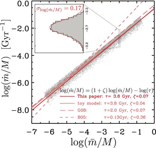
Orbit-averaged mass-loss rate, |$\dot{m}$|, as a function of the orbit-averaged subhalo mass, |$\bar{m}$|, both normalized by the mass of the host halo, M. Grey dots indicate the 10 000 individual Monte Carlo realizations of the toy model (see Appendix B) for a host halo mass of M = 1013 h− 1M⊙. Red lines of different styles represent equation (1) with parameters advocated by B05 (thin, short-dashed), G08 (thin, long-dashed), our toy model (thin, solid) and our final, tuned model (thick, solid). Inset: the distribution of orbit-averaged mass-loss rates at |$\log (\bar{m}/M)=-2$|, which is well represented by a lognormal distribution with dispersion |$\sigma _{\log (\dot{m}/M)} = 0.17$| (red curve).
The thin, long-dashed, red line in Fig. 2 shows the best-fitting relation of G08. Although in fairly good agreement with our toy model, it has a slightly steeper slope (ζ = 0.07), and a higher normalization (|${\cal A}= 1.54$|).2 In addition, G08 also measured a somewhat larger scatter of |$\:\sigma _{\log {\cal A}}\simeq 0.25$|. It is important to realize, though, that G08 measured the subhalo mass-loss rates over a time interval of ∼0.1 Gyr, which is much shorter than the typical radial period of (infalling) subhaloes (5 Gyr ≲ Tr ≲ 9 Gyr). Hence, the G08 results do not properly reflect the orbit-averaged mass-loss rates. In fact, since the mass-loss rate can vary dramatically along any individual orbit, their scatter is expected to be larger than for our toy model, and this may also impact the average normalization. As for the slope, the (small) discrepancy with respect to our toy model might be a manifestation of dynamical friction, which causes enhanced mass-loss rates for the more massive subhaloes. Hence, since our toy model does not include a treatment of dynamical friction, it is likely to underestimate ζ. Indeed, as we show in Section 3.2, when tuning our model, we find that ζ = 0.07 is a better match to the simulation data than ζ = 0.04.
2.3 The structural evolution of subhaloes
In addition to subhalo mass, we also want the semi-analytical model to predict the maximum circular velocity, Vmax, for each of its subhaloes.
Both relations are obtained using idealized simulations, and it is worth checking whether they are accurate in a cosmological setting. Fig. 3 compares both fitting functions against results from the Bolshoi, Rhapsody and ELVIS simulations (see Section 3 for descriptions), all of which have been analysed using the rockstar (Behroozi, Wechsler & Wu 2013a; Behroozi et al. 2013b) halo finder.3 Whereas the simple Vmax ∝ m1/3 relation advocated by Hayashi et al. (2003) is clearly incompatible with the cosmological simulations, the P10 relation is an excellent fit. There is some indication that it overpredicts Vmax/Vacc at small m/macc, but this is most likely a manifestation of limited force resolution in the cosmological simulations. In what follows, we therefore model the Vmax/Vacc − m/macc relation using equation (9) with (η, μ) = (0.3, 0.4).
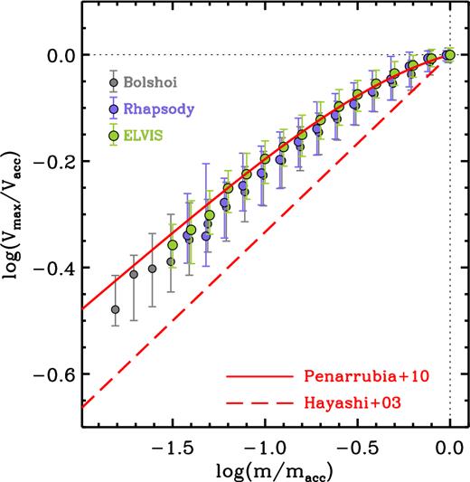
The ratio Vmax/Vacc as function of retained mass fraction m/macc. The solid, red line is the relation of Peñarrubia et al. (2010) that we use to compute the maximum circular velocities of dark matter subhaloes in our semi-analytical model. Circles represent the median relations obtained from various simulations, as indicated, with error bars indicating the 16 and 84 percentiles. The dashed, red line indicates the Vmax ∝ m1/3 relation advocated by Hayashi et al. (2003).
Note that the simulation results reveal a significant amount of scatter in Vmax/Vacc at given m/macc. This is contrary to the P10 results, which find the relation to be virtually scatter free. However, P10 did not account for scatter in the concentrations of host and subhaloes. We have checked whether the Vmax/Vacc–m/macc scatter in the cosmological simulations is correlated with halo concentrations, but did not find any (see also Emberson, Kobayashi & Alvarez 2015). Instead, as shown in Paper II, we find that the same simulation when processed with different halo finders, can yield very different median Vmax/Vacc–m/macc relations. We therefore expect that the scatter in the cosmological simulations is mainly a manifestation of noise in the mass estimates of dark matter subhaloes, and we use the P10 relation with zero scatter to compute the maximum circular velocities of subhaloes in our model. We have verified that explicitly adding scatter in the Vmax/Vacc–m/macc relation similar to that seen in Fig. 3 does not have a significant impact on any of our results.
2.4 Subhalo disruption
During each pericentric passage, a subhalo experiences a tidal shock (e.g. Spitzer 1987; Gnedin & Ostriker 1997) which impulsively heats the subhalo, and eventually may lead to its complete disruption. Unfortunately, whether subhaloes ever get completely disrupted, and under what circumstances, is still a matter of debate. For example, Hayashi et al. (2003) find that subhaloes disrupt once their tidal radius, rt, becomes smaller than ∼2rs,acc, while Diemand et al. (2007) argue that even subhaloes with rt < 0.2rs,acc survive in the Via Lactea simulation. Here rs,acc = rvir/cacc is the NFW scale radius at accretion. Other studies argue that, in a pure dark matter universe, without any dense baryonic components, the central NFW-like cusp of subhaloes will actually resist disruption indefinitely (e.g. Goerdt et al. 2007; Peñarrubia et al. 2010). The main reason for this lack of consensus is that the numerical simulations and halo finders used to study subhalo disruption suffer from limiting mass and force resolution. Consequently, as a subhalo loses mass, it becomes more and more sensitive to numerical artefacts.
Rather than treating fdis as a free parameter, we instead use the Bolshoi simulation for guidance. Using the publicly available Bolshoi halo catalogues, it is straightforward to identify subhaloes that are to be disrupted (hereafter TBD) as the subhaloes that have no descendants in all subsequent time steps.4 At each of the outputs examined, the fraction of subhaloes that are identified as TBD is only ∼0.1 per cent. Although this may seem insignificant, the total fraction of subhaloes that experience disruption accumulates over time and can become very substantial. Indeed, as we demonstrate in Section 3.2, including a treatment of subhalo disruption is essential, at least if one aims to reproduce the subhalo populations in numerical simulations.
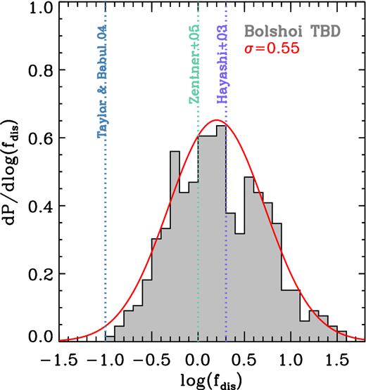
The distribution of fdis, a measure of the effective disruption radius, of the to-be-dirupted subhaloes in the Bolshoi simulation (dark grey), which can be approximated by a lognormal distribution with standard deviation |$\:\sigma _{\log (f_{\rm dis})}=0.55$| and median |$\bar{f}_{\rm dis}=1.6$| (red curve). The vertical, dotted lines mark the fixed values of fdis used in previous studies, as indicated.
In our model, we treat tidal disruption by drawing, for each individual subhalo, a value of fdis from the lognormal of equation (11), and disrupting the subhalo once its mass drops below the critical mass given by equation (10). We emphasize that this disruption model is entirely guided by results from the Bolshoi simulation, and that the model is therefore subject to the same shortcomings as the simulation. In particular, as mentioned above, disruption in numerical simulations may largely be a numerical artefact. We leave the discussion as to whether tidal disruption is physical or not to a future paper, in which we focus on how tidal disruption, or the lack thereof, impacts a number of astrophysical topics. Here, we focus on modelling the evolution of dark matter substructure such that the model is able to reproduce the simulation results.
2.5 Computing subhalo mass and velocity functions
Having described all the ingredients, we now outline how these are combined to compute the subhalo mass and velocity functions for a target host halo of mass M0 at redshift z0. We first construct a merger tree, with a mass resolution of ψres = 10−5, as described in Section 2.1. Next, we follow each trajectory forward in time, starting from the redshift zacc at which the trajectory's halo first becomes a subhalo, evolving the subhalo mass in between merger-tree time steps, using the subhalo mass-loss rate given by equations (1)–(3) for which the normalization |${\cal A}$| is a trajectory-specific random variable drawn from the lognormal distribution of equation (5) with median |$\bar{{\cal A}}$|. For each trajectory, we also draw a value for fdis from the lognormal distribution of equation (11). This sets the trajectory-specific threshold mass mdis. When the subhalo's mass m(t) drops below mdis, it is removed from the inventory, and all its sub-subhaloes are released to the parent halo.
For each subhalo, we compute the maximum circular velocity at accretion, Vacc, using the following approach. We first use the merger tree to compute t0.04, the time at which the subhalo's most massive progenitor first reaches a mass equal to 4 per cent of its mass at accretion. If the mass of the subhalo at the leave point of its trajectory is larger than 0.04 macc, we use the P08 algorithm to extent the trajectory's MAH further back in time until the main progenitor mass drops below 0.04 macc. Once t0.04 has been obtained, we compute Vacc using equations (6)–(8). Once the subhalo is accreted, the evolution of its maximum circular velocity is computed using equation (9) with (η, μ) = (0.3, 0.4).
Note that we loop over trajectories sorted by increasing order, which assures that each subhalo is evolved in its properly evolved, direct parent halo. In particular, if a first-order subhalo of mass m1 is orbiting within a zeroth-order parent halo of mass m0, and hosts a second-order subhalo (i.e. a sub-subhalo) of mass m2, the latter is evolved using equation (3) with M = m1 and m = m2, while m1 is evolved using the same equation but with M = m0 and m = m1. We ignore both subhalo–subhalo mergers, as well as the possibility that a higher order subhalo is stripped from its direct parent. As discussed in Paper II and van den Bosch et al. (in preparation), these oversimplified assumptions have a negligible impact on the accuracy of our model.
Our model is characterized by a total of five parameters: |$\bar{{\cal A}}$|, |$\:\sigma _{\log {\cal A}}$| and ζ describe the average mass-loss rate of subhaloes, while |$\bar{f}_{\rm dis}$| and |$\:\sigma _{\log (f_{\rm dis})}$| characterize tidal disruption. Each of these parameters has a well-motivated value. For the mass-loss model, these come from the toy model described in Section 2.2, according to which |$\bar{{\cal A}} = 0.81$|, |$\:\sigma _{\log {\cal A}}= 0.17$| and ζ = 0.04. For the tidal disruption model, we are guided by the results from the Bolshoi simulation, according to which |$\bar{f}_{\rm dis}= 1.6$| and |$\:\sigma _{\log (f_{\rm dis})}= 0.55$|. These are the values we adopt for our ‘primary model’. As we show in Section 3.2 below, only a small amount of fine tuning of some of these parameters is required in order to accurately reproduce the subhalo mass and SHVFs in the Bolshoi simulation.
3 RESULTS
Our model as described above yields, at each redshift, the evolved mass and Vmax for all orders of subhaloes. In this section, we compare the predictions from our primary model with simulation results, and slightly tune some of the parameters in order to accurately match the SHMF in the Bolshoi simulation for host haloes with M0 ≃ 1014.2 h− 1M⊙. Next we show that the same model accurately reproduces the subhalo mass and velocity functions for other host halo masses, and discuss how the abundance of subhaloes scales with halo mass and redshift. However, we start with a brief description of the numerical N-body simulations used for comparison with our model predictions.
3.1 N-body simulations
The main simulation that we use to calibrate and test our model is the Bolshoi simulation (Klypin, Trujillo-Gomez & Primack 2011), which follows the evolution of 20483 dark matter particles in a box of size 250 h−1Mpc using the Adaptive Refinement Tree (art) code (Kravtsov, Klypin & Khokhlov 1997). The simulation adopts a flat ΛCDM cosmology with parameters |$(\Omega _{\rm m},\Omega _\Lambda , \Omega _{\rm b},h,\sigma _8, n_{\rm s})=(0.27,0.73,0.047,0.7,0.82,0.95)$| (hereafter ‘Bolshoi cosmology’), and has a particle mass of mp = 1.35 × 10⁸ h− 1M⊙. We use the publicly available halo catalogues5 obtained using the phase-space halo finder rockstar (Behroozi et al. 2013a,b). rockstar haloes are defined as spheres with an average density of Δvirρcrit.
In addition to the Bolshoi simulation, we also use the ELVIS suite6 of 48 MW-size dark matter haloes (Garrison-Kimmel et al. 2014a), and the Rhapsody suite7 of 96 cluster-sized dark matter haloes (Wu et al. 2013a,b). Both are sets of high-resolution, zoom-in simulations, with a particle mass of mp = 1.35 × 10⁵ and 1.3 × 10⁸ h− 1M⊙, respectively, and have been analysed using the same rockstar halo finder. More details regarding these simulations can be found in Paper II and in the references given.
3.2 Model calibration
3.2.1 Primary model
In order to test and calibrate our model, we start by comparing the results predicted by our primary model, for which |$(\bar{{\cal A}}, \:\sigma _{\log {\cal A}}, \zeta , \bar{f}_{\rm dis}, \:\sigma _{\log (f_{\rm dis})}) = (0.81, 0.17, 0.04, 1.6, 0.55)$|, with results from the Bolshoi simulation. For the comparison, we use all 281 Bolshoi haloes with M0 = 1014.25 ± 0.25 h− 1M⊙ and 2000 model realizations for a halo mass of M0 = 1014.2 h− 1M⊙ in the Bolshoi cosmology. This mass range is chosen as a compromise between sample size and dynamic range: for smaller M0 the number of host haloes in the Bolshoi simulation is larger, but due to the limiting mass resolution, the dynamic range in subhalo mass is smaller.
Results are shown in Fig. 5, where the filled circles indicate the evolved, cumulative SHMF, N(> m/M0), in the Bolshoi simulation. The solid, blue line is the corresponding prediction from our primary model, which is in good agreement with the simulation results at the low-mass end, but somewhat overpredicts the number of massive subhaloes. The open circles and the long-dashed blue lines are the simulation and model results for what we call the unevolved, surviving SHMF, which indicates the abundance of surviving subhaloes as function of their mass at accretion. Note that this is different from the unevolved SHMF, which indicates the abundance of all subhaloes, irrespective of whether they survive to the present or not. For comparison, the latter is indicated as the red, short-dashed line, and is very different from the unevolved, surviving SHMF. As we will see below, the difference marks the impact of tidal disruption.
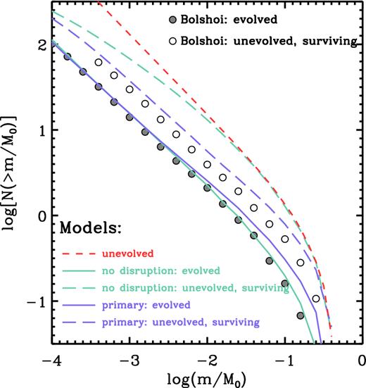
The average, cumulative SHMFs from the primary model (blue) and the model with no disruption (cyan). Model predictions (lines), averaged over 2000 realizations of halo mass M0 = 1014.2 h− 1M⊙, are compared with the Bolshoi results (symbols) averaged for all 281 host haloes in the mass bin M0 = 1014.25 ± 0.25 h− 1M⊙. The solid lines and filled symbols represent the evolved SHMFs; the long dashed lines and open circles represent the unevolved, surviving SHMFs; and the short dashed, red line represents the unevolved SHMF, which is the same for the primary and the ‘no disruption’ models as it reflects only the merger trees rather than the subhalo mass evolution.
Similar as for the evolved SHMF, the primary model also overpredicts the evolved, surviving SHMF. Hence, we need to modify the model by either increasing the amount of stripping, or by increasing the likelihood of disruption. Fortunately, there is no degeneracy between these options; as it turns out, there is only one combination of stripping and disruption that can simultaneously reproduce the evolved and the unevolved, surviving SHMFs. To illustrate this, we have constructed a model without tidal disruption that we tuned to reproduce the evolved SHMF. The result is shown as the green lines, and has |$(\bar{{\cal A}}, \:\sigma _{\log {\cal A}}, \zeta , \bar{f}_{\rm dis}, \:\sigma _{\log (f_{\rm dis})}) = (1.55, 0.17, 0.09, 0.0, 0.0)$|. Although this model accurately reproduces the evolved SHMF, it dramatically overpredicts the unevolved, surviving SHMF. In fact, in a model without disruption, the unevolved, surviving SHMF is identical to the unevolved SHMF of all subhaloes (red, short-dashed line), except for the difference at the low-mass end which is due to incompleteness (we only include subhaloes with present-day mass m ≥ 10−4M0). This demonstrates the importance of treating tidal disruption. The magnitude of tidal disruption is consistent with that found by Han et al. (2016), using the Aquarius simulations.
Fig. 6 shows three more diagnostics. The shaded histogram in the left-hand panel shows the distribution of the retained mass fraction, m/macc, for present-day subhaloes in the Bolshoi simulation.8 The fraction of subhaloes with m/macc < 0.1 is only ∼5 per cent, while there are basically no subhaloes for which m/macc < 0.01. On average, a surviving subhalo retains ∼60 per cent of its mass at accretion. The m/macc distribution predicted by the primary model is in reasonable agreement with the simulation results, although it slightly overpredicts the abundance of subhaloes with small retaining mass fractions. The ‘no-disruption’ model predicts a pronounced tail that extends well below m/macc = 0.01, in clear disagreement with the simulation results, and it also has a deficit of subhaloes with m/macc > 0.3. This once more highlights the necessity of modelling subhalo disruption. Tests show that the median of the m/macc distribution is sensitive to the parameter |$\bar{f}_{\rm dis}$|, while a scatter of |$\:\sigma _{\log (f_{\rm dis})}\simeq 0.55$| is essential for reproducing the low-m/macc tail.
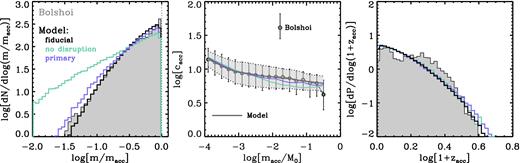
Key diagnostics for model calibration: the distribution of the retained mass fraction (left), the concentration at accretion as a function of mass at accretion (middle), and the distribution of accretion redshifts (right), for present-day, surviving subhaloes. These results are based on all the 281 host haloes of masses M0 = 1014.25 ± 0.25 h− 1M⊙ in the Bolshoi simulation, or 2000 model realizations of halo mass M0 = 1014.2 h− 1M⊙. Overplotted in cyan are the predictions from a model without disrupting subhaloes but with enhanced mass-loss such that it can reproduce the evolved SHMF almost equally well compared to the fiducial model (black). In the middle panel, the filled circles (solid line) represent the median, with the error bars (shaded band) indicating the 16 and 84 percentile of the Bolshoi (model) result.
The middle panel of Fig. 6 plots the concentration at accretion, cacc, for present-day subhaloes, as a function of the mass at accretion normalized by the present-day host halo mass, macc/M0. The primary model slightly underpredicts the concentrations for subhaloes with macc/M0 ≳ 0.003, but otherwise is in good agreement with the simulation results. Reproducing these accretion concentrations is essential for accurately reproducing the SHVFs. After all, cacc sets the maximum circular velocity at accretion, Vacc, which in turn determines Vmax of the surviving subhaloes via equation (9). Note that the discrepancy between model and simulation results becomes significantly larger for the no-disruption model. This is because less concentrated subhaloes are more easily disrupted than their more concentrated counterparts: disruption boosts the median cacc of the surviving subhaloes.
Finally, the right-hand panel of Fig. 6 plots the distribution of accretion redshifts for the present-day subhaloes, which shows that the vast majority of the surviving subhaloes were accreted at zacc ≲ 2. The model predictions are overall in good agreement with the Bolshoi result, both for the primary model as well as for the model without disruption. As we demonstrate in Appendix C, the zacc distribution is fairly sensitive to |$\:\sigma _{\log {\cal A}}$|, with larger scatter resulting in zacc-distributions with more extended tails to high zacc. Using the zacc-distribution of subhaloes in the Bolshoi simulation, we infer that |$\:\sigma _{\log {\cal A}}\lesssim 0.25$|, which comfortably includes the fiducial value, |$\:\sigma _{\log {\cal A}}=0.17$|, suggested by our toy model.
Note that the zacc-distribution in the Bolshoi simulation reveals a dip around zacc ∼ 0.25 that is not reproduced by our models. As shown in van den Bosch et al. (2014), this dip is an artefact arising from the fact that subhaloes in the simulation have to be located within the virial radius, rvir, of their host. Subhaloes that were accreted around zacc ∼ 0.25 are at the present close to their first apocentric passage, which for a large fraction of subhaloes falls outside of rvir. Hence, the dip reflects the temporary ‘ejection’ (or ‘splashback’) of subhaloes that are actually bound to the host halo (see e.g. Gill, Knebe & Gibson 2005; Sales et al. 2007; Ludlow et al. 2009).
3.2.2 Fiducial model
It is clear that tidal disruption is an essential ingredient of our model, and that the primary model does a very reasonable job in reproducing a wide range of diagnostics regarding the statistics of subhaloes. However, there is room for improvement, and we now proceed by tuning some of the model parameters to achieve a better fit to the evolved and unevolved, surviving SHMFs. We find that keeping |$\:\sigma _{\log {\cal A}}=0.17$| while changing |$\bar{{\cal A}}$| from 0.81 to 0.86 and ζ from 0.04 to 0.07 yields an evolved SHMF in excellent agreement with the Bolshoi results. This only represents a change of 6 per cent in the normalization, while the change in the slope ζ is more or less expected from the fact that our toy model ignores dynamical friction (see discussion in Section 2.2). Interestingly, ζ = 0.07 is in excellent agreement with the value inferred by G08 from directly measuring the mass-loss rates in numerical simulations. As we demonstrate in Appendix C, there is a substantial degeneracy between the values of |$\bar{{\cal A}}$| and |$\:\sigma _{\log {\cal A}}$|: we can increase the normalization |$\bar{{\cal A}}$| and simultaneously increase the scatter |$\:\sigma _{\log {\cal A}}$| and yield subhalo mass and velocity functions that are indistinguishable. This means that the specific values adopted for our fiducial model, |$(\bar{{\cal A}},\:\sigma _{\log {\cal A}}) = (0.86,0.17)$|, have some freedom.
The resulting model predictions for the retained mass fractions, the halo concentrations at accretion and the accretion redshifts are shown as grey lines in Fig. 6. Note that this tuned model (hereafter ‘fiducial model’) clearly improves upon the primary model, and accurately reproduces each of these three key statistics.
Fig. 7 compares the predictions of our fiducial model (grey lines) to the average, cumulative SHMFs, N(>m/M0) and SHVFs, N(>Vmax/Vvir, 0), in the Bolshoi simulation, for three different bins in host halo mass (symbols). Here Vvir, 0 is the host halo's virial velocity at z0 = 0. From left to right, the panels show the simulation results for host haloes with M0 = 1012.7±0.01 (571 haloes), 1013.5±0.05 (441 haloes) and 1014.25 ± 0.25 h− 1M⊙ (281 haloes), respectively. These are compared to model predictions that are obtained by averaging the results from 2000 Monte Carlo realizations for host haloes with M0 = 1012.7, 1013.5 and 1014.2 h− 1M⊙. We have verified that the halo mass bins are narrow enough, and do not introduce noticeable systematics in the mass and Vmax functions.
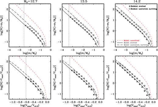
The average, cumulative SHMFs, N(>m/M0) (upper) and SHVFs, N(>Vmax/Vvir, 0) (lower). Model predictions (lines), averaged over 2000 realizations of halo masses M0 = 1012.7 (left), 1013.5 (middle) and 1014.2 h− 1M⊙ are compared with the Bolshoi results (symbols) averaged for all the 571, 441 and 281 host haloes in the corresponding mass bin M0 = 1012.7±0.01, M0 = 1013.5±0.05 and M0 = 1014.25 ± 0.25 h− 1M⊙. The solid lines and filled symbols represent the evolved SHMFs (SHVFs). The long-dashed lines and open symbols represent the unevolved, surviving SHMFs (SHVFs), i.e. the abundance of surviving subhaloes as function of their mass (Vmax) at accretion. The short-dashed lines are the model predictions of the unevolved SHMFs (SHVFs), i.e. the abundance of all subhaloes ever accreted to the host halo's main progenitor, as function of mass (Vmax) at accretion. Overplotted in cyan lines only for halo mass M0 = 1014.2 h− 1M⊙ are the predictions from the model without subhalo disruption, but with enhanced mass-loss relative to the fiducial model so that it can also roughly reproduce the Bolshoi evolved SHMF.
The agreement between model and simulation results is very good, for all the different mass and velocity functions shown. We emphasize that our fiducial model is calibrated using only the SHMFs from the 281 host haloes in the Bolshoi simulation with M0 = 1014.25 ± 0.25 h− 1M⊙. Yet, it nicely reproduces the mass and velocity functions for all mass bins shown. In particular, it performs equally well for the evolved SHMFs and SHVFs (solid dots plus solid lines) as for the unevolved, surviving SHMFs and SHVFs (open dots plus long-dashed curves). As demonstrated above, this indicates that our model accurately reproduces the tidal disruption in the Bolshoi simulation. The fact that the unevolved SHMF and SHVF for the surviving subhaloes are so different from those for all subhaloes (red, short-dashed curves) once again indicates that tidal disruption is extremely important, at least in the Bolshoi simulation. The model slightly overpredicts the velocity functions in the regime where N(>Vmax/Vvir, 0) < 1. However, we refrain from overinterpreting this discrepancy, because simulation results are limited by the uncertainty of halo finders in dealing with major mergers (Behroozi et al. 2015), and different simulation results easily differ by a factor of a few in this regime (see Paper II).
Thus far we have demonstrated that the fiducial model accurately captures the mass dependence of the subhalo mass and velocity functions. We now turn our attention to the redshift dependence. We first obtain the average, evolved SHMFs of Bolshoi haloes with mass M0(z0) = 1012.75±0.25 and 1013.75 ± 0.25 h− 1M⊙, at z0 = 0, 0.2, 0.5, 1.0, and compare these to our model predictions for haloes with mass M0(z0) = 1012.7 and 1013.7 h− 1M⊙. All these SHMFs have the same shape, but different normalizations (see also Angulo et al. 2009; Giocoli et al. 2010, and Section 4 below). This normalization-redshift dependence is shown in Fig. 8, which plots the SHMF, dN/dlog [m/M0(z0)], at fixed log [m/M0] = −2 as a function of redshift z0. For both mass scales, the model predictions (lines) are in good agreement with the simulation results (filled circles). We find a similar degree of agreement for the redshift dependence of the unevolved, surviving SHMFs as well as the SHVFs (not shown for brevity). We therefore conclude that our fiducial model yields subhalo mass and velocity functions that accurately match the Bolshoi results as function of both halo mass and redshift.
![Comparison of the redshift dependence of the evolved SHMFs of the model and that of the Bolshoi simulation: dN/dlog [m/M0(z0)] at log [m/M0] = −2 for Bolshoi haloes with mass M0(z0) = 1012.75±0.25 and 1013.75 ± 0.25 h− 1M⊙, compared with the model predictions for haloes with mass M0(z0) = 1012.7 and 1013.7 h− 1M⊙. The fixed halo masses used for the model predictions correspond to the average masses of the haloes in the mass bins used for the simulation results, and we have verified that a bin width of 0.5 dex has negligible effect on the average SHMF.](https://oup.silverchair-cdn.com/oup/backfile/Content_public/Journal/mnras/458/3/10.1093_mnras_stw439/2/m_stw439fig8.jpeg?Expires=1749849740&Signature=KRPa6IeZbYeFFs1mroO~1N-OveSaAg5BUyxUFvgJDQ4h3Oi0ivEWDXJPNJrFwWFVh1rjWCS0QFd5v1Iu5HU0R7L1ITRepysWmlXFMCIUqvwxiKtAkQwLvubc~XObfEYVcbUa6ie-lDBefpLHyNCXVT68RKKFs87SrLpZue4kfwotUyfZEMFYXRMZqSh9JegHqMEiX0KOp87aVohiD9x-D7QWlFffT8gfBR5guGJRVOUjl04afGZb3FuReWwKwvnmnfdf5iAS6HfdK~gxQnFnl4Pu1WISIyRz6pXNgbf3jmZke8mBJCDBfXhaQV2fC7HXozkPWBvs5wDc-ZLpOn9uQg__&Key-Pair-Id=APKAIE5G5CRDK6RD3PGA)
Comparison of the redshift dependence of the evolved SHMFs of the model and that of the Bolshoi simulation: dN/dlog [m/M0(z0)] at log [m/M0] = −2 for Bolshoi haloes with mass M0(z0) = 1012.75±0.25 and 1013.75 ± 0.25 h− 1M⊙, compared with the model predictions for haloes with mass M0(z0) = 1012.7 and 1013.7 h− 1M⊙. The fixed halo masses used for the model predictions correspond to the average masses of the haloes in the mass bins used for the simulation results, and we have verified that a bin width of 0.5 dex has negligible effect on the average SHMF.
3.3 Mass, order and redshift dependence
Having calibrated and tested our model, we now explore in more detail how the subhalo mass and velocity functions depend on host halo mass, redshift and subhalo order. To this end, we compute the average, differential SHMFs, dN/dlog (m/M0), and SHVFs, dN/dlog (Vmax/Vvir, 0), averaged over 10 000 Monte Carlo realizations, for host haloes of masses log [M0/(h−1 M⊙)] = 11, 12, …, 15, and redshifts z0 = 0, 1, 3 and 5 in the Bolshoi cosmology.
The upper left-hand panel of Fig. 9 plots the z0 = 0 SHMFs for the five different host halo masses. Solid and dashed curves correspond to the evolved and unevolved SHMFs. It is well known that the unevolved SHMF is universal, i.e. independent of host halo mass, redshift or cosmology (see e.g. Lacey & Cole 1993; B05; Li & Mo 2009; Yang et al. 2011). The evolved SHMFs on the other hand, are mass dependent with the normalization increasing with increasing host halo mass. This halo mass dependence, first noticed in numerical simulations by Gao et al. (2004) and in semi-analytical models by B05, simply reflects the fact that more massive haloes assemble later. Haloes that assemble later accrete their subhaloes later, which in turn are subjected to tidal stripping and tidal disruption for a shorter period of time. Note that the universality of the unevolved SHMF indicates that, on average, all haloes accrete subhaloes of the same, normalized mass.
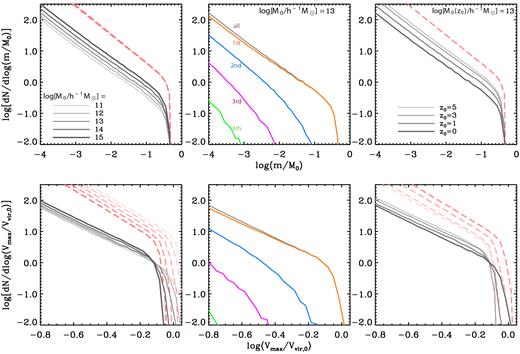
Average SHMFs (upper) and SHVFs (lower) obtained by averaging over 10 000 merger trees each. Left-hand panel: the unevolved (dashed) and evolved (solid) subhalo mass and velocity functions of different host halo masses. Middle: the evolved mass and velocity functions of subhaloes of different orders, for host halo mass M0 = 1013 h− 1M⊙. Right-hand panel: the unevolved (dashed) and evolved (solid) subhalo mass and velocity functions for halo mass M0 = 1013 h− 1M⊙ at different redshifts as indicated.
The upper-middle panel of Fig. 9 plots the z0 = 0 SHMFs for subhaloes of different orders, for host haloes of mass M0 = 1013 h− 1M⊙. Note that as the order increases by one, the normalization reduces by roughly an order of magnitude, while the slope steepens. The grey line shows the SHMF of all orders, which is clearly completely dominated by first-order subhaloes. Note though that the slope of the SHMF of all orders is slightly steeper than that of first-order subhaloes (see Section 4).
The upper right-hand panel of Fig. 9 plots the SHMFs of all orders for host haloes of mass M0 = M0(z0) = 1013 h− 1M⊙ at different redshifts z0. Host haloes at higher redshifts have a larger abundance of subhaloes than host haloes of the same mass at lower redshifts. As mentioned before, the unevolved SHMF is universal and therefore also independent of redshift.
The lower panels of Fig. 9 are the same as the upper ones, but for the SHVFs. Overall the trends are very similar except for one important difference: the unevolved SHVFs are not universal. As is evident from the lower left-hand and lower right-hand panels, the overall normalization of the unevolved SHVF increases with decreasing host halo mass and decreasing redshift. As discussed in Section 4 below, this is a consequence of the concentration–mass–redshift relation of dark matter haloes, which causes a cross-over in the mass and redshift dependence of the evolved SHVFs at the massive end. Not shown in Fig. 9 are the unevolved, surviving subhalo mass/velocity functions, which exhibit qualitatively the same mass, order and redshift dependence as their evolved counterparts, but with a somewhat higher normalization.
All together it is easy to understand the mass, redshift and even cosmology dependence by considering the following. As discussed in B05, the subhalo mass fraction of a given halo at redshift z is a trade-off between the time-scale, τacc, on which new subhaloes are being ‘accreted’ by the host halo, and the time-scale, |$\tau =\tau _{\rm dyn}/{\cal A}\simeq \tau _{\rm dyn}$|, of subhalo mass-loss. The latter evolves with redshift as described by equation (2), and therefore was shorter in the past. The former depends on the MAH of the host halo, and is thus a function of both redshift and halo mass. In the limit where τacc ≪ τdyn, subhalo mass-loss is negligible and the normalization of the SHMF will increase with time, asymptoting towards the unevolved SHMF. The opposite limit, in which τacc > τdyn, is equivalent to that of subhalo mass-loss in a static parent halo. In this case, the normalization of the SHMF will decrease with time. Since τacc is of the order of the Hubble time, which is always larger than the dynamical time of a halo, we are typically in the latter regime, in which the normalization of the SHMF decreases with decreasing redshift, and in which more massive haloes have more substructure. The latter simply follows from the fact that more massive haloes assemble later, and therefore have a larger τacc. The only exception to this rule of thumb are the very early stages of halo formation, when halo growth is extremely fast and τacc ≃ τdyn.
4 UNIVERSAL MODELS FOR THE SUBHALO MASS AND VELOCITY FUNCTIONS
Fig. 9 suggests that the evolved SHMFs have a universal shape, with a normalization that depends on halo formation time. This universality has its origin in the universal shape of the unevolved SHMF, and suggests that it should be straightforward to obtain a fitting function for the evolved SHMF, dN/dln (m/M0), that is valid for different M0, z0 and cosmologies. In fact, similar universal fitting functions may also be found for the evolved and unevolved velocity functions, as well as the unevolved, surviving subhalo mass and velocity functions.
In order to have a sufficient dynamic range to probe the mass and cosmology dependence, we construct the average SHMFs and SHVFs for host haloes spanning the mass range |$10^{11} \:h^{-1}\rm M_{\odot }\le M_0 \le 10^{15} \:h^{-1}\rm M_{\odot }$| in cosmologies that span the range 0.1 ≤ Ωm ≤ 0.5, 0.5 ≤ σ8 ≤ 1.0 and 0.5 ≤ h ≤ 1.0. Our ‘standard’ model is for a host halo of mass M0 = 1013 h− 1M⊙ in the Bolshoi cosmology with (Ωm, h, σ8) = (0.27, 0.7, 0.82), which falls roughly mid-way of the ranges considered. When varying cosmology, we only vary one of these three parameters at a time, relative to the standard model, and compute the average SHMF and SHVF for host haloes with M0 = 1011 and 1015 h− 1M⊙ averaging over 20 000 Monte Carlo realizations at redshift z0 = 0.
Before presenting the results, we caution that the ‘universal model’ presented below is based on the ansatz that our fiducial model, which we only thoroughly tested against the Bolshoi simulation, remains valid for cosmologies other than that used for Bolshoi. This implies that we assume that the effective model parameters, that describe the mass stripping and tidal disruption (equations 1 and 12), are independent of cosmology. In our model, the SHMFs and SHVFs are the outcome of a competition between accretion (as described by the halo merger trees) and the dynamical evolution of subhaloes (e.g. mass stripping and tidal disruption). The cosmology dependence of halo merger trees is accounted for via the EPS-based formalism used. The dynamical evolution of subhaloes is taken to scale with the dynamical time, τdyn, which itself is cosmology and redshift dependent (see equation 2). Since the evolution of subhaloes is a purely gravitational process, which is scale-free, there is no obvious reason why any of the effective parameters should depend on cosmology. However, until this is explicitly tested using large numerical simulations, similar to Bolshoi, but for a broad range of cosmologies, we caution that the universal model presented below may be less accurate for cosmologies that differ substantially from the ΛCDM cosmology adopted for the Bolshoi simulation. In fact, we only advocate using the ‘universal model’ to describe subhalo mass and velocity functions in ΛCDM cosmologies with parameters that are roughly consistent (within a factor of ∼2) with current constraints. The reason is that our merger trees rely on the P08 correction to the EPS PMF, which was originally calibrated using the Millennium simulations ((Ωm, h, σ8, n) = (0.25, 0.73, 0.8, 1)). Although JB14 have shown that the P08 correction is also valid for slightly different ΛCDM cosmologies, it has not been tested yet for more deviant cosmologies.
4.1 Unevolved SHMF (ψ = macc/M0)
As shown in Li & Mo (2009) and JB14, one can use the universality of the unevolved SHMF of first-order subhaloes to compute that of nth order subhaloes. Since first-order subhaloes can themselves be considered as host haloes at the time of accretion, their subhaloes, which are of second order, are also expected to follow the universal, unevolved SHMF. Consequently, the unevolved SHMF for second-order subhaloes can simply be obtained by convolving that of first-order subhaloes with itself, and the same logic applies for higher orders (see JB14 for details). For the unevolved SHMF of all orders, one can sum up the unevolved SHMFs of all different orders n = 1, 2, …. In practice, the sum of the first three orders is sufficient, as the contribution from even higher orders is negligible, at least for subhaloes with m > 10−5M0. We find that this ‘all-order’ unevolved SHMF is well fitted by equation (13) with parameters (γ, α, β, ω) = (0.22, −0.91, 6, 3).
4.2 Evolved SHMF (ψ = m/M0)
The upper panels of Fig. 10 plot the SHMFs for host haloes of mass M0 = 1011 and 1015 h− 1M⊙ for the six most extreme cosmologies considered here. The left, middle and right-hand columns show the results for first-order subhaloes, second-order subhaloes, and subhaloes of all-orders, respectively. The dashed, red curves are the corresponding universal unevolved SHMFs. Note that the evolved SHMFs have similar shapes, but with normalizations that differ by up to ∼1 dex.
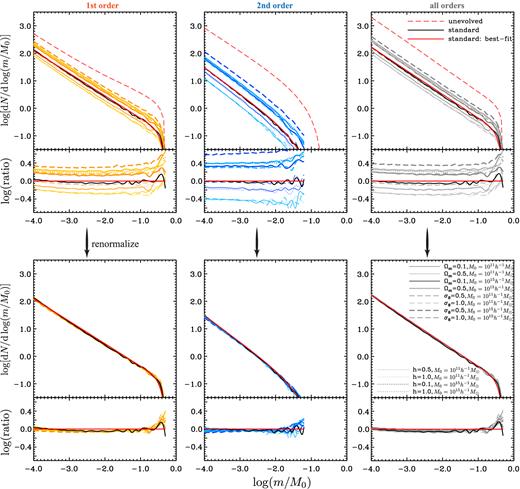
Upper row: the average SHMFs, for subhaloes of the first order (left), second order (middle), and all orders (right), at redshift z = 0 for different cosmologies and host halo masses, as indicated. The dashed, light-red curves represent the universal unevolved SHMFs. The solid black curves represent the standard model for a host halo of mass M0 = 1013 h− 1M⊙ in the Bolshoi cosmology. The solid, red curves are the fitting functions of the form of equation (13) that best fits the standard model. The small panels show the ratios with respect to this best fit to the standard model. Lower row: same as the upper row, but this time the SHMFs have been renormalized by their subhalo mass fraction, fs (see text for details).
The halo mass dependence of the evolved SHMF has already been discussed in Section 3.3, where we have shown that the normalization of the mass function increases with the mass of the host halo. Here we focus on the cosmology dependence. Upon inspection of the upper row of Fig. 10, one can discern that lower Ωm yields stronger M0 dependence: for host haloes of mass M0 = 1015 h− 1M⊙ (thicker lines), lowering Ωm causes an increase in the normalization of the SHMF; while for host haloes of mass M0 = 1011 h− 1M⊙ (thinner lines), the effect flips sign. The Ωm dependence enters via its effect on the assembly history of the host halo. Decreasing Ωm makes the formation time earlier (later) for more massive (less massive) host haloes, with the pivot point around M0 ∼ 1013 h− 1M⊙ (see van den Bosch 2002; Giocoli, Tormen & Sheth 2012). As discussed in relation to the halo mass dependence, an earlier (later) assembly of the host halo results in present-day subhalo populations that are more (less) depleted due to tidal stripping. Similarly, higher σ8 implies earlier assembly, and therefore lower normalization of the evolved SHMFs. The Hubble constant, h, has negligible effect on the assembly history over the range probed here (see Giocoli et al. 2012), and therefore does not have a significant impact on the evolved SHMFs.
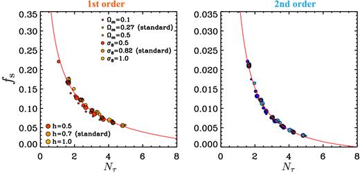
The relation between subhalo mass fraction, fs, and the host halo's ‘dynamical age’, Nτ, defined as the number of dynamical time-scales elapsed since the formation of the (average) host halo (see equation 17). The left- and right-hand panels correspond to first- and second-order subhaloes, respectively. Symbols of different size and shades indicate different cosmologies. For each cosmology, there are five points, corresponding to the five halo masses, log (M0/ h− 1M⊙) = 11, 12, …, 15. The red lines are the best-fitting relations given by equations (19) and (20).
The above relations between fs and Nτ allow one to compute the average, evolved SHMF for a halo of any mass, at any redshift and for a wide range of ΛCDM cosmologies. Direct comparison with numerical simulations is hampered by the fact that the differences in simulations are dominated by differences in the (sub)halo finders used (see Paper II). In a recent paper, however, Dooley et al. (2014) studied how varying cosmological parameters impacts the abundance of subhaloes using a series of simulations that were all analysed with the same rockstar halo finder. They find that changing σ8, ns and Ωm over the ranges [0.7, 0.9], [0.9, 1.0] and [0.19, 0.35], respectively, results in changes of the SHMFs of MW-sized host haloes that are small compared to the halo-to-halo variance, and argue that cosmology dependence can therefore be ignored. According to our universal fitting function, the normalization of the SHMF for σ8 = 0.7 is 24 per cent higher than for σ8 = 0.9, that for ns = 0.9 is 10 per cent higher than for ns = 0.9, and that for Ωm = 0.19 is 17 per cent higher than for Ωm = 0.35 for host haloes of mass M0 = 1012 h− 1M⊙. In an era of precision cosmology, we do not consider differences of such a magnitude insignificant. We emphasize that our results are consistent with those presented in Dooley et al. (2014), to the extent we can judge. Unfortunately, the authors do not quote any errors on the average SHMFs. Since they used simulations with a tiny box size of only 25 h−1 Mpc, we expect this error to be about as large as the differences predicted by our model. In addition, Dooley et al. overestimated the halo-to-halo variance by stacking results for host haloes that span a large range in host halo mass; a significant component of their halo-to-halo variance is simply due to the host-halo mass dependence of the SHMF.
4.3 The unevolved subhalo velocity function (ψ = Vacc/Vvir, 0)
Having shown that universal fitting functions exist for both the evolved and unevolved SHMFs, we now examine whether similar, universal functions exist to describe the evolved and unevolved SHVFs. The convenient universality present in the case of the unevolved mass function does not hold for the velocity function. This is easy to understand from the fact that the relation between macc and Vacc = Vmax(zacc) depends on the concentration–mass–redshift relation. The ‘mapping’ of macc/M0 into Vacc/Vvir, 0 therefore depends on mass, redshift and cosmology.
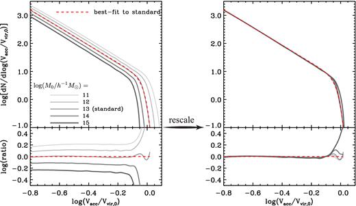
Left-hand panel: the average, unevolved SHVFs, dN/dlog (Vacc/Vvir, 0), for different host halo masses in the Bolshoi cosmology. The red curve represents the fitting function of the form of equation (21) that best fits the standard model (i.e. M0 = 1013 h− 1M⊙). The bottom panel plots the ratios relative to this fitting function. Right-hand panel: same as for the left-hand panel, except that here the SHVFs have been rescaled using the scale parameter a given by equation (23).
We have experimented with different values for f, and obtain the best results for f = 0.25, for which C = 1.536. The right-hand panels of Fig. 12 plot dN/dlog (Vacc/Vvir, 0) versus a Vacc/Vvir, 0, where a is computed using equation (23) with these values. This simple rescaling almost completely captures the halo mass dependence in the unevolved SHVF, making the rescaled functions almost indistinguishable from each other and well fitted by equation (21) with α = −3.2, β = 2.2, γ = 2.05, ω = 13 and a = 1 (red curve). Some discrepancies that go beyond statistical noise are evident at the high-velocity end, but only for the most massive host haloes. Although the discrepancies are within a factor of 2, we caution that the ‘universal’ unevolved SHVF presented here is less reliable for the most massive subhaloes in the most massive (cluster-sized) host haloes.
We have verified that the same scale parameter a (with f = 0.25) also captures the cosmology and redshift dependences. There is a weak dependence of the power-law slope α on cosmology, but this only becomes cumbersome when the cosmological parameters deviate substantially (i.e. by about a factor of 2 or more) from the Bolshoi cosmology with (Ωm, h, σ8) = (0.27, 0.7, 0.82). Overall the rescaling proposed here allows one to compute reliable, unevolved SHVFs for host haloes of different mass, at different redshifts, and for a broad range of ΛCDM cosmologies.
4.4 The evolved SHVF (ψ = Vmax/Vvir, 0)
The left-hand panels of Fig. 13 plot the evolved SHVFs corresponding to the unevolved SHVFs shown in Fig. 12. As with the evolved mass functions, the slope of the evolved SHVFs is independent of host halo mass, and the normalization increases with increasing M0. However, at the high-Vmax end, the halo mass dependence flips over, with the transition to the exponential decay occurring at smaller Vmax/Vvir, 0 for more massive host haloes. As we demonstrate in Paper II, these trends are consistent with the results from N-body simulations.
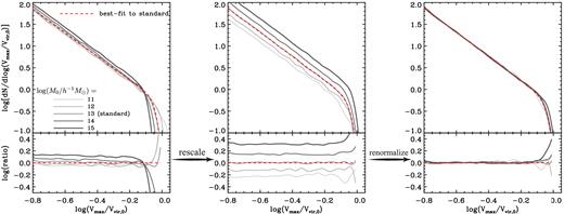
Left: the average, evolved SHVFs, dN/dlog (Vmax/Vvir, 0) for different halo masses in the Bolshoi cosmology. Middle: after rescaling with the parameter a, the flip-over in the halo mass dependence at the high-Vmax end is gone, and the evolved SHVFs have a universal shape, but different normalizations. Right: further renormalizing the rescaled, evolved SHVFs by |$f_{\rm s}^{1.25}$| collapses them together, bringing them in good agreement with the best fit (red line, see text) to the standard model.
In an attempt to construct a universal fitting function for the evolved SHVF, we first apply the rescaling that successfully captures the mass dependence of the unevolved SHVF. This results in the rescaled, evolved SHVFs shown in the middle panels of Fig. 13. The exponential decay now occurs at roughly the same scale, i.e. the ‘cross-over’ present in the left-hand panels is removed. The dependence of the normalization on host halo mass now resembles that of the evolved SHMF, which reflects the effect of subhalo mass evolution. Hence, we expect that this normalizations scales with the halo's dynamical age, Nτ. Recall that, in the case of the evolved SHMF, the normalization constant is simply proportional to the subhalo mass fraction fs. In the case of the evolved SHVF, we find, by trial and error, that the normalization scales with |$f_{\rm s}^{1.25}$|. This is demonstrated in the right-hand panels of Fig. 13, which indicates that renormalization by |$f_{\rm s}^{1.25}$| yields SHVFs that are almost indistinguishable. This universal, evolved SHVF is well described by equation (21) with (γ, α, β, ω) = (0.195, −2.77, 4.6, 17.8). As with the unevolved SHVF, small discrepancies are evident at the high-Vmax end, but overall, this two-stage process of rescaling and renormalization nicely captures the mass dependence of the evolved SHVF. We have verified that this process also captures the cosmology and redshift dependences.
4.5 Unevolved, surviving SHMF (ψ = macc/M0)
For completeness, we also provide fitting functions for the unevolved, surviving subhalo mass and velocity functions, which are defined as the mass and velocity functions of the surviving (i.e. not-disrupted) subhaloes at their epoch of accretion. We emphasize that these functions are of particular interest, as they provide the basis for the popular technique of subhalo abundance matching, in which galaxy properties such as luminosity or stellar mass get assigned to dark matter subhaloes in numerical simulations based on their mass or maximum circular velocity at infall (e.g. Conroy et al. 2006; Vale & Ostriker 2006; Conroy & Wechsler 2009; Behroozi, Conroy & Wechsler 2010; Hearin et al. 2013).
We find that the unevolved, surviving SHMF can be well fitted by equation (13) with a universal (α, β, ω) = (−0.87, 40, 5). As discussed in Section 3.2, the difference between the unevolved SHMF and the unevolved, surviving SHMF reflects subhalo disruption, which in our model occurs whenever the subhalo mass drops below some critical value (see Section 2.4). Hence, in an ensemble-averaged sense, disruption is simply a manifestation of mass stripping, and we therefore expect that the normalization of the unevolved, surviving SHMF scales with the subhalo mass fraction fs. By trial and error we find that this dependence is accurately captured by |$\gamma \propto f_{\rm s}^{0.7}$| (see Appendix A for details).
4.6 The unevolved, surviving SHVF (ψ = Vacc/Vvir, 0)
Finally, the universal fitting function for the unevolved, surviving SHVF, can be based on that for the evolved SHVF. In analogy, consider the case of the unevolved, surviving mass function relative to the evolved mass function: their fitting functions are similar, except that the normalization constant γ of the former has a weaker dependence on the mass fraction fs. Therefore, the same two-stage fitting process for the evolved SHVF should also be applicable to the unevolved, surviving SHVF, except that in the second stage, the renormalization factor should be a weaker function of fs. Indeed, we find that using |$\gamma \propto f_{\rm s}^{0.95}$| as the renormalization factor accurately describes the normalization dependence of the unevolved, surviving SHVFs. For more details, see Appendix A.
5 SUMMARY
We have presented a new semi-analytical model that uses EPS merger trees to generate evolved subhalo populations. The model is based on the method pioneered by B05, and evolves the mass of dark matter haloes using a simple model for the orbit-averaged subhalo mass-loss rate. This avoids having to integrate individual subhalo orbits, as done in other semi-analytical models for dark matter substructure (e.g. Benson et al. 2002; Taffoni et al. 2003; Zentner & Bullock 2003; Oguri & Lee 2004; Taylor & Babul 2004, 2005a,b; Peñarrubia & Benson 2005; Zentner et al. 2005; Gan et al. 2010). We have made a number of improvements and extensions to the original B05 model. In particular, we
use Monte Carlo merger trees constructed using the method of P08, which, as demonstrated in JB14, yields results in much better agreement with numerical simulations than the SK99 method used by B05;
construct and use complete merger trees, rather than just the mass assembly histories of the main progenitor. This allows us to investigate the statistics of subhaloes of different orders;
adopt a new mass-loss model that accounts for the scatter in subhalo mass-loss rates arising from scatter in orbital properties (energy and angular momentum) and (sub)halo concentrations;
include a method for converting halo mass to maximum circular velocity, thus allowing the model to predict SHVFs as well as SHMFs;
add a treatment of subhalo disruption that is carefully calibrated against numerical simulations.
Our model has five parameters, each of which has a well-motivated value; either from a simple toy model, in the case of tidal stripping, or from numerical simulations, in the case of tidal disruption. The ‘primary’ model based on these parameters already yields subhalo statistics that are in fairly good agreement with simulation results. We have tuned some of the parameters to more accurately reproduce the SHMFs for host haloes with M0 ≃ 1014.2 h− 1M⊙ in the Bolshoi simulation. The resulting ‘fiducial’ model accurately reproduces SHMFs and SHVFs for other host halo masses, yields mass and velocity functions for subhaloes of any order, and is applicable to any viable ΛCDM cosmology.
The unevolved SHMF is (almost) independent of host halo mass, redshift and cosmology (see also Lacey & Cole 1993; B05; Li & Mo 2009; Yang et al. 2011). We emphasize, though, that although the functional form of equation (24) can adequately describe this universal unevolved SHMF, it is more accurately described by the double-Schechter-like function presented in JB14.
The evolved SHMF has a universal shape accurately described by equation (24), with a normalization, γ, that depends on host halo mass, redshift and cosmology. We have demonstrated that γ is tightly correlated with the ‘dynamical age’ of the host halo, defined as the number of halo dynamical times that have elapsed since its formation. Using this relation we have presented a universal fitting function for the average, evolved SHMF that is valid for any host halo mass, at any redshift, and for any ΛCDM cosmology. A similar fitting formula exists for the unevolved, surviving SHMF, except that its normalization has a weaker dependence on the dynamical age than the evolved SHMF.
Unlike the unevolved SHMF, the unevolved SHVF is not universal, in that the parameter β depends on host mass, redshift and cosmology. This has its origin in the concentration–mass–redshift relation of dark matter haloes, and can be accounted for by replacing ψ in equation (24) with aψ, where a is a (universal) scale factor given by a ∝ Vvir(M0/40, z0)/Vmax(M0/40, z0.25). Using this simple rescaling, one obtains a universal fitting function for the unevolved SHVF for which the parameters α, β, γ and ω are all independent of host mass, redshift and cosmology.
Taking into account both the ‘dynamical age’ dependence of the normalization of the evolved SHMF and the ‘a’ scaling of the unevolved SHVF, also yields universal fitting functions for the evolved and the unevolved, surviving SHVFs, whereby the latter has a weaker dependence on the dynamical age.
The various, universal fitting functions for the subhalo mass and velocity functions presented here, and summarized in Appendix A, can be used to quickly compute the average abundance of subhaloes of given mass or maximum circular velocity, at any redshift, and for any (reasonable) ΛCDM cosmology, without having to run and analyse high-resolution numerical simulations. They can be used, among others, to rescale simulation results, to predict or rescale conditional stellar mass or luminosity functions, or to compute the occupation statistics of dark matter subhaloes.
In the second paper in this series (Paper II), we compare subhalo mass and velocity functions obtained from different simulations and with different subhalo finders, among each other, and with predictions from our semi-analytical model. We demonstrate that our model is in excellent agreement with simulation results that analyse their data with halo finders that use phase-space information and temporal information. Results obtained using subhalo finders that only rely on the densities in configuration space are shown to dramatically overpredict the slope of subhalo mass/velocity functions. In Paper III (Jiang & van den Bosch in preparation), we use our model to quantify the halo-to-halo variance of dark matter substructure at unprecedented precision. In particular, we characterize the scatter in subhalo mass fraction and subhalo occupation numbers.
The model presented here can be used in a number of astrophysical applications. As an example, in Jiang & van den Bosch (2015), we have used it for a comprehensive assessment of the TBTF problem. Using thousands of realizations of MW size host haloes, we investigated the statistics used to characterize the TBTF problem in unprecedented detail. We also demonstrated in that paper that the halo-to-halo variance predicted by our model is in excellent agreement with that found in numerical simulations.
We are grateful to Peter Behroozi, for updating the Bolshoi halo catalogue upon our request, to Hao-Yi Wu for sharing data from the Rhapsody simulation project, and to the anonymous referee for an insightful report that greatly helped to improve the presentation. We also thank the organizers of the programme ‘First Galaxies and Faint Dwarfs: Clues to the Small Scale Structure of Cold Dark Matter’ held at the Kavli Institute for Theoretical Physics (KITP) in Santa Barbara, for creating a stimulating, interactive environment that started the research presented in this paper, and the KITP staff for all their help and hospitality. This research was supported in part by the National Science Foundation under Grant No. PHY11-25915.
These simulations cover host haloes with masses ranging from M0 ∼ 1012.1 to 1014.8 h− 1M⊙. We have verified that the Vmax/Vacc–m/macc relation has no halo mass dependence. Since gravity is scale-free, and haloes are self-similar structures, this is expected.
At each simulation output, TBD subhaloes are identified in the halo catalogue as having an ‘mmp’ flag equal to 0.
The halo catalogues of the ELVIS suite are publicly available at http://localgroup.ps.uci.edu/elvis/data.html.
The Rhapsody halo catalogue is kindly provided by Hao-Yi Wu.
We find the corresponding distributions in the ELVIS and Rhapsody simulation suites to be statistically indistinguishable.
Actually, we sample the circularities from the modified distribution, |${\cal P}(\eta )\, {\rm d}\eta = {\pi \over 2}\, \sin (\pi \eta ) \, {\rm d}\eta$|, which accurately fits equation (B10) and has the advantage that it allows values of η to be drawn by direct inversion.
We have verified that drawing subhalo mass from the unevolved SHMF instead does not alter any of the results.
REFERENCES
APPENDIX A: UNIVERSAL FITTING FUNCTIONS FOR THE SUBHALO MASS AND VELOCITY FUNCTIONS
Fitting function parameters.
| Type | ψ | γ | α | β | ω | a |
|---|---|---|---|---|---|---|
| Unevolved SHMF | macc/M0 | 0.22 | −0.91 | 6 | 3 | 1 |
| Evolved SHMF | m/M0 | 0.280fs | −0.86 | 50 | 4 | 1 |
| Unevolved, surviving SHMF | macc/M0 | |$0.286f_{\rm s}^{0.7}$| | −0.87 | 40 | 5 | 1 |
| Unevolved SHVF | Vacc/Vvir, 0 | 2.05 | −3.2 | 2.2 | 13 | equation (A3) |
| Evolved SHVF | Vmax/Vvir, 0 | |$3.717 f_{\rm s}^{1.25}$| | −2.77 | 4.6 | 17.8 | equation (A3) |
| Unevolved, surviving SHVF | Vacc/Vvir, 0 | |$3.095 f_{\rm s}^{0.95}$| | −2.87 | 2 | 15 | equation (A3) |
Note. Parameters for the universal fitting functions of the form equation (A1) for different ‘types’ of subhalo mass and velocity functions for subhaloes of all orders. The parameter fs is defined as the fraction of the host halo mass that is locked up in subhaloes with mass m > 10−4M0. (see equation 15).
In what follows, we outline the steps required to compute the values of fs and a for a host halo of mass M0 at redshift z0 in a given ΛCDM cosmology.
- Obtain the redshift zf, by which the main progenitor has assembled a fraction f of its final mass M0 at redshift z0. In particular, compute zf for f = 0.5, 0.25 and 0.04 using the G12 model for formation redshift, by solving for the root ofwhere |$\tilde{w}_f = \sqrt{2\ln (\alpha _f + 1)}$| and |$\alpha _f = 0.815\,e^{-2f^3}\!/\!f^{0.707}$|.(A2)\begin{equation} \delta _{\rm c}(z_f) = \delta _{\rm c}(z_0) + \tilde{w}_f \sqrt{\sigma ^2(fM_0)-\sigma ^2(M_0)}, \end{equation}
Compute the ‘dynamical age’, Nτ, of the host halo using equation (17) with zform = z0.5. Use this to infer the subhalo mass fraction, fs, from equation (19).
- Compute the parameter, a, given bywith Vvir and Vmax given by equations (7) and (6), respectively, and with z0.25 obtained in step (i). Note that the computation of Vmax requires the halo concentration parameter, c, which can be computed from the z0.04 obtained under step (i) using the concentration–mass–redshift relation of Zhao et al. (2009), given by equation (8).(A3)\begin{equation} a = 1.536 \, {V_{\rm vir}(M_0/40,z_0) \over V_{\rm max}(M_0/40,z_{0.25})}, \end{equation}
Although we believe these fitting functions to be accurate for host haloes that cover a wide range in halo masses and redshifts, and for a wide range of cosmologies, we caution that we have only been able to test them against numerical simulations over the mass range |$10^{12} \:h^{-1}\rm M_{\odot }\lesssim M_0 \lesssim 10^{15}\:h^{-1}\rm M_{\odot }$| at relatively low redshifts, and for a range of cosmologies that are all similar to the best-fitting cosmologies advocated by the recent CMB experiments (see Paper II for details). We therefore caution against using this method blindly for cosmologies and/or halo masses that are very different from those mentioned above.
APPENDIX B: SUBHALO MASS-LOSS RATES: A TOY MODEL
An important goal of this work is to assess the halo-to-halo variance of subhalo statistics (discussed in more detail in Paper III and Jiang & van den Bosch 2015). The main source of this variance is the scatter in mass accretion histories, which is accounted for via our merger trees. However, another potentially important source of scatter is that due to the variance in the orbital properties; orbits with more negative orbital energy, or with smaller angular momentum, will have a smaller pericentre and therefore experience more tidal stripping. In addition, since the tidal radius of a subhalo depends on the density profiles of host halo and subhalo, a third source of scatter is the variance in halo concentrations, of both the host halo and the subhalo.
Using numerical simulations, G08 indeed found a substantial scatter in the subhalo mass-loss rates, which is well represented by a lognormal with a standard deviation of |$\sigma _{\log (\dot{m}/M)} \sim 0.25$|. However, G08 measured the mass-loss rates averaged over a time step of ∼0.1 Gyr, which is much shorter than an orbital period. Hence, their mass-loss rates are not truly orbit-averaged, and their scatter contains a contribution due to variations in |$\dot{m}/M$| along individual orbits. In order to gauge the scatter in orbit-averaged subhalo mass-loss rates due to the variance in orbital properties and halo concentrations we consider a simple, but insightful, toy model.
Consider a subhalo of mass m on an orbit of energy E and angular momentum L (both per unit mass) inside a host halo of mass M. In what follows we use r and R to refer to subhalo-centric and host halo-centric radii, respectively. As the subhalo orbits within the potential of the host halo, it experiences dynamical friction, tidal heating and tidal stripping, all contributing to the mass-loss indirectly or directly. Assuming most of the mass-loss occurs close to the orbit's pericentre, Rp, where the tidal field of the host is strongest, we may approximate the orbit-averaged mass-loss rate with equation (4), which assumes that all the mass beyond the tidal radius of the subhalo at the orbit's pericentre is stripped from the subhalo in one radial period. As we have shown in Section 2.2, this simplified model yields results in close agreement with numerical simulations.
Using this toy model, we compute orbit-averaged mass-loss rates for large ensembles of subhaloes as follows. For a given host halo mass, we first draw a subhalo mass, m, from a uniform distribution10 on the interval log (m/M) ∈ [ − 6.0, −0.5]. Next, we draw concentrations for both the host halo and subhalo from the lognormal distribution described above, and draw orbital circularity and energy from the distributions given by equations (B10) and (B11). These are used to compute the radial orbital period, Tr, and the subhalo's tidal radius, rt, from which we ultimately compute the mass-loss rate using equation (4). Results are described in Section 2.2.
APPENDIX C: DEGENERACY BETWEEN |$\bar{{\cal A}}$| AND |$\:\sigma _{\log {\cal A}}$|
Our model for the subhalo mass-loss rate has three free parameters: a normalization |$\bar{{\cal A}}$|, a scatter |$\:\sigma _{\log {\cal A}}$| and a slope ζ. The simple toy model of Section 2.2 suggests that |$\bar{{\cal A}} = 0.81$|, |$\:\sigma _{\log {\cal A}}=0.17$| and ζ = 0.04. After tuning our model to the Bolshoi simulation results, we adjust the parameters to |$\bar{{\cal A}} = 0.86$|, |$\:\sigma _{\log {\cal A}}=0.17$| and ζ = 0.07. Here we explore potential degeneracy among these parameters.
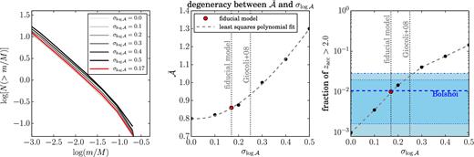
Degeneracy between the normalization of the average mass-loss rate, |$\bar{{\cal A}}$| and the scatter |$\:\sigma _{\log {\cal A}}$|. Left-hand panel: the evolved SHMFs with different |$\:\sigma _{\log {\cal A}}$| (grey lines). The red line corresponds to our fiducial model (|$\:\sigma _{\log {\cal A}}=0.17$|) and is shown for comparison. Middle panel: the best-fitting |$\bar{{\cal A}}$| as a function of |$\:\sigma _{\log {\cal A}}$|, for models with |$\:\sigma _{\log {\cal A}}$| indicated in the left-hand panel, and |$\bar{{\cal A}}$| adjusted to reproduce the fiducial, evolved SHMF. The dashed line indicates the least-squares polynomial fit to the degenerate sets of |$(\bar{{\cal A}}, \:\sigma _{\log {\cal A}})$|, given by equation (C1), while vertical, dotted lines mark the scatter of our fiducial model, and that measured from numerical simulations by G08. Right-hand panel: fraction of subhaloes (in host haloes with M0 ∼ 1014.2 h− 1M⊙) that have an accretion redshift zacc > 2.0 as a function of |$\:\sigma _{\log {\cal A}}$|. The horizontal, blue dashed line indicates the fraction of such subhaloes in the Bolshoi simulation, with the shaded regions indicating the 68 and 95 confidence intervals (computing assuming Poisson statistics). Symbols correspond to our model predictions, and are consistent with the Bolshoi results (at 95 per cent CL) as long as |$\:\sigma _{\log {\cal A}}\lesssim 0.25$|.
This degeneracy freedom in the model implies that there is some room for the interpretation of the parameters |$\bar{{\cal A}}$| and |$\:\sigma _{\log {\cal A}}$|. This is important, given that our model makes the oversimplified assumption that subhaloes lose mass at a constant rate. Although this is a fair description of what happens to subhaloes on circular orbits, subhaloes on more radial orbits will have mass histories, m(t), that are more reminiscent of a step function, with virtually all mass-loss occurring close to pericentre (see e.g. Taylor & Babul 2004; Peñarrubia et al. 2010). Our model does not account for this subperiod variation in subhalo mass-loss rates, and therefore underestimates the variance in subhalo masses at any given epoch. In order to estimate how this might impact our results, we consider the extreme case in which each subhalo has a m(t) that, each radial period, evolves as a step function: if in our fiducial model the subhalo mass decreases continuously from m0 to m1 over a period T, then now we have m(t) = m0 for t ≤ T/2 and m(t) = m1 for t > T/2. With the same mass-loss parameters as for our fiducial model, this modified model yields an evolved SHMF with a higher normalization. However, we can offset this by increasing either |$\bar{{\cal A}}$| or |$\:\sigma _{\log {\cal A}}$|. In particular, we find that this extreme mass-loss model yields results that are indistinguishable from our standard model if we increase |$\bar{{\cal A}}$| from 0.86 to 1.0, or, equivalently, we increase |$\:\sigma _{\log {\cal A}}$| from 0.17 to 0.3. Since the typical orbit of a subhalo is neither circular nor radial, the typical subhalo will have a mass-loss history, m(t), that falls somewhere in between the two extremes discussed above. The upshot is that our subhalo mass-loss model is to be considered an ‘effective’ model that accounts for the subperiod variations in subhalo mass-loss rates, even though we do not explicitly model those variations.
