


Abstract
We study the distribution and evolution of the stellar mass and the star formation rate (SFR) of the brightest group galaxies (BGGs) over 0.04 < z < 1.3 using a large sample of 407 X-ray galaxy groups selected from the COSMOS, AEGIS, and XMM–LSS fields. We compare our results with predictions from the semi-analytic models based on the Millennium simulation. In contrast to model predictions, we find that, as the Universe evolves, the stellar mass distribution evolves towards a normal distribution. This distribution tends to skew to low-mass BGGs at all redshifts implying the presence of a star-forming population of the BGGs with MS ∼ 1010.5 M⊙ which results in the shape of the stellar mass distribution deviating from a normal distribution. In agreement with the models and previous studies, we find that the mean stellar mass of BGGs grows with time by a factor of ∼2 between z = 1.3 and z = 0.1, however, the significant growth occurs above z = 0.4. The BGGs are not entirely a dormant population of galaxies, as low-mass BGGs in low-mass haloes are more active in forming stars than the BGGs in more massive haloes, over the same redshift range. We find that the average SFR of the BGGs evolves steeply with redshift and fraction of the passive BGGs increases as a function of increasing stellar mass and halo mass. Finally, we show that the specific SFR of the BGGs within haloes with M200 ≤ 1013.4 M⊙ decreases with increasing halo mass at z < 0.4.
1 INTRODUCTION
Brightest groups/cluster galaxies (here after BGGs) are generally located at the core of the hosting haloes and close to the centre of the extended X-ray emitting hot intragroup/cluster medium. Their privileged location within the group/cluster and their stellar luminosity makes them ideal targets for constraining cosmological models and studying the assembly histories of massive galaxies (Sandage 1972, 1976; Gunn & Oke 1975; Bhavsar & Barrow 1985; Hoessel & Schneider 1985; Oegerle & Hoessel 1991; Postman & Lauer 1995; Bernstein & Bhavsar 2001; Bernardi et al. 2007; De Lucia & Blaizot 2007; von der Linden et al. 2007; Liu et al. 2009; Stott et al. 2010).
BGGs are generally early-type galaxies with no significant ongoing star formation. They differ from other massive galaxies in surface brightness profiles and scaling relations (e.g. Graham et al. 1996; Bernardi et al. 2007; von der Linden et al. 2007; Liu et al. 2008). These findings suggest that formation of the BGGs could be different from that of other normal elliptical galaxies (e.g. Collins & Mann 1998; Burke, Collins & Mann 2000; Stott et al. 2008, 2010; Wen & Han 2011; Méndez-Abreu et al. 2012; Shen et al. 2014).
Understanding the stellar mass assembly of galaxies, particularly BGGs, is highly important for galaxy formation and evolution scenarios and thus has been the focus of a number of studies based on the hierarchical assembly of the dark matter haloes in the Λ cold dark matter (ΛCDM) cosmology (e.g. White & Rees 1978; Voit 2005; Tutukov, Dryomov & Dryomova 2007); halo abundance matching simulations (e.g. Moster, Naab & White 2013); the semi-analytic model (SAM) of galaxy formation (e.g. Bower et al. 2006; Croton et al. 2006; De Lucia & Blaizot 2007; Guo et al. 2011; Tonini et al. 2012; Gonzalez-Perez et al. 2014; Cousin et al. 2015; Merson et al. 2016); and the observational studies as well (e.g. Stott et al. 2010; Lin et al. 2013; Oliva-Altamirano et al. 2014).
Previous studies indicate that the evolutionary history of galaxies in terms of the mass growth can be divided into two main epochs. A very early epoch, above z ∼ 2, in which the star formation rate (SFR) is peaked and the majority of stars (∼80 per cent) in the BGGs form due to the rapid cooling from their hot and dense haloes (e.g. Hopkins & Beacom 2006; De Lucia & Blaizot 2007). A later epoch, SFR declines possibly because the cold stream is suppressed by shock heating (Dekel et al. 2009). The stellar and AGN feedback may have played a role as well. Furthermore, strong ram-pressure stripping of the interstellar medium and the tidal fields of groups and clusters contributed to the quenching. By this stage, the BGGs have considerably grown in mass and they generally follow a passive evolution (e.g. Croton et al. 2006; Conroy, Wechsler & Kravtsov 2007; Liu et al. 2010; Stott et al. 2010).
Using near-infrared luminosity as a proxy for stellar mass, some studies determined the growth of the stellar mass in BGGs, claiming that these systems exhibit little/no changes in mass below z ∼ 1 (Collins & Mann 1998; Whiley et al. 2008; Collins et al. 2009; Stott et al. 2010). In contrast, some recent studies have argued that the stellar mass of the BGGs have grown due to galaxy mergers by a factor of ∼2 between z ∼ 1 and z ∼ 0.2 (De Lucia & Blaizot 2007; Lidman et al. 2012; Lin et al. 2013; Bai et al. 2014). These contradicting results demonstrate that the details of the stellar mass assembly of BGGs still remain elusive. The main purpose of this paper is to take advantage of a large sample of X-ray detected groups and their BGGs to study the stellar mass evolution over the last ∼9 billions years of the age of the Universe.
SAMs have become a standard tool to help us interpret observations and place constraints on the formation and evolution of galaxies. Using a SAM based on the Millennium simulation (Springel et al. 2005), De Lucia & Blaizot (2007) traced back the formation history of the central cluster galaxies within dark matter haloes and pictured their full merger trees. They found that significant fraction of stars (50 per cent and 80 per cent) in the central luminous galaxy form at high redshifts (above z ∼ 3 and z ∼ 2) and half of their final mass is carried by a single galaxy below z ∼ 0.5. Since then, they grow through major mergers and a significant number of the minor mergers. Furthermore, Lin et al. (2013), using a sample of the BGGs selected from the Spitzer IRAC Shallow Cluster Survey with halo mass range of (2.4–4.5) × 1014, found that these galaxies have grown by a factor of 2.3 between z = 1.5 and z = 0.5. While the predictions from Guo et al. (2011) SAM agrees well with these observations, below z < 0.5 the model fails to reproduce the observed growth.
Moreover, Liu et al. (2010) studied the stellar mass of central and satellite galaxies selected from the galaxy group catalogues in the Sloan Digital Sky Survey and the three SAMs, and found that all models fail to reproduce the sharp decrease in the stellar mass with decreasing halo mass at the low-mass end while models also overpredict the number of satellites by roughly a factor of 2. Furthermore, we have shown that SAMs fail to match the observed evolution of the relation between the magnitude gap between the first the second BGGs, and their intrinsic luminosity (Smith et al. 2010; Gozaliasl et al. 2014). Thus, the SAMs still requires further improvement and more sophisticated treatment of the physical processes, which is often performed via tuning a large number of parameters (Benson 2010). However, they still serve as a reasonable guide, we compare three SAMs based on the Millennium simulation presented in Bower et al. (2006, hereafter B06), De Lucia & Blaizot (2007, hereafter DLB07), and Guo et al. (2011, hereafter G11) with the observations.
In this paper, we analyse a large sample of the X-ray galaxy groups and clusters selected from the XMM–LSS (Gozaliasl et al. 2014), COSMOS (Finoguenov et al. 2007; George et al. 2011), and AEGIS (Erfanianfar et al. 2013) fields in a wide redshift range 0.04 < z < 1.3. Most of the previous studies have focused on the evolution of the brightest galaxies within massive clusters with masses above M200 ∼ 1014 M⊙. Our sample covers a lower mass range between M200 ∼ 1012.8 and 1014 M⊙. This allows us to study the galaxy assembly in more common environments in the universes.
This paper is structured as follows. We define data and describe how we infer galaxy stellar mass in Section 2. In Section 3, we present the distribution and evolution of the stellar mass of the BGGs. Section 4, presents an analysis of the distribution of the SFR in the BGGs and its dependence on stellar/halo mass. Section 5 is a summary of our results.
Unless stated otherwise, we adopt a cosmological model, with (ΩΛ, ΩM, h) = (0.75, 0.25, 0.71), where the Hubble constant is characterized as 100 h km s−1 Mpc−1 and quote uncertainties on 68 per cent confidence level.
2 GROUP SAMPLE
2.1 Subsample definition
We use the combined data of the X-ray galaxy groups and clusters from three surveys, XMM–LSS, COSMOS, and AEGIS, which have been presented in details in Gozaliasl et al. (2014), Finoguenov et al. (2007), George et al. (2011), and Erfanianfar et al. (2013). These catalogues include 456 galaxy groups/clusters with halo masses ranging from M200 ∼ 5 × 10¹² to 1014.5( M⊙) over a redshift range of 0.04 < z < 1.9.
Over 70 per cent of all galaxy groups in our data have spectroscopic redshifts. For the purpose of our study and to ensure a high accuracy photometric redshift measurement, we limit the sample to the redshift range of 0.04 ≤ z ≤ 1.3 and halo mass range of M200 ≃ 7.25 × 10¹² to 1.04 × 10¹⁴( M⊙), namely galaxy groups. This selection provides us with a sample of 407 X-ray groups. The left upper panel of Fig. 1 illustrates the halo mass (M200) as a function of the group redshift. This plane allows us to define five subsamples as follows:
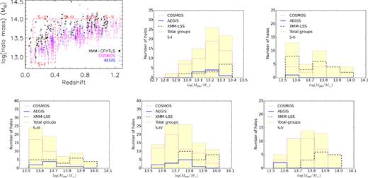
Left upper panel: M200 as a function of the redshift for the X-ray galaxy groups selected from the COSMOS (open magenta diamonds), XMM–LSS (filled black circles), and AEGIS (open blue triangles) fields. The dashed red boxes present our five defined subsamples as described in Section 2.1. All panels except the left upper panel: the halo mass distribution of the total number of galaxy groups within each subsample (filled yellow histogram) and those selected from the COSMOS (dashed magenta histogram), XMM–LSS (solid black histogram), and AEGIS (dotted blue histogram) fields.
(S-I) 0.04 < z < 0.40 and |$12.85 {<} {\rm log}(\frac{M_{200}}{\,\mathrm{M}_{{\odot }}}) \le 13.40$|
(S-II) 0.10 < z ≤ 0.4 and |$13.50 {<} {\rm log}(\frac{M_{200}}{\,\mathrm{M}_{{\odot }}}) \le 14.02$|
(S-III) 0.4 < z ≤ 0.70 and |$13.50 {<} {\rm log}(\frac{M_{200}}{\,\mathrm{M}_{{\odot }}}) \le 14.02$|
(S-IV) 0.70 < z ≤ 1.0 and |$13.50 {<} {\rm log}(\frac{M_{200}}{\,\mathrm{M}_{{\odot }}}) \le 14.02$|
(S-V) 1.0 < z ≤ 1.3 and |$13.50 {<} {\rm log}(\frac{M_{200}}{\,\mathrm{M}_{{\odot }}}) \le 14.02$|
The defined subsamples (hereafter, S-I to S-V) include 74, 36, 63, 92, and 48 galaxy groups, respectively. The M200–z plane enables us to adopt a similar halo mass range for the last four subsamples (S-II to S-V). The halo mass range for these subsamples is narrow (<0.5 dex). The average uncertainty associated with the mass estimate of our sample of galaxy groups is about 0.17 ± 0.1 dex. In Fig. 1, we separately show the halo mass distribution for all subsamples of galaxy groups and those selected from the COSMOS (dashed magenta histogram), XMM–LSS (solid black histogram), and AEGIS (dotted blue histogram) fields. The halo mass distribution for the total number of the galaxy groups within S-II to S-V peaks around log(M200/M⊙) ∼ 13.7 ± 0.2. For S-II and S-III, the peak of distribution tends to skew lower masses. However, we repeat our analysis several times with considering different halo mass ranges for the last four subsamples and find that the small bias towards high halo masses at high redshifts falls within errors and does not affect our results. Thus, this also makes it possible to investigate the evolutionary properties of the BGGs over 0.1 < z < 1.3.
In this paper, we compare observations with predictions from three SAMs (G11, DLB07, and B06) based on the Millennium simulation. For detailed information on these models, we refer reader to G11, DLB07, and B06. We note that some important properties of these models have been summarized in Gozaliasl et al. (2014). We randomly select our subsamples of galaxy groups from the SAM catalogues according to the redshift and halo mass limits which defined for the sample of the galaxy groups in observations.
2.2 BGG selection
We first identify member galaxies with spectroscopic redshift and then include likely member galaxies with red sequences with a help of multiband photo-z's. The galaxy photometric redshift catalogues are from Ilbert et al. (2013), McCracken et al. (2012), Capak et al. (2007, COSMOS), Brimioulle et al. (2008, 2013, XMM–LSS), and (Wuyts et al. 2011, AEGIS), and the red sequences finder can be found in Mirkazemi et al. (2015). From the member catalogues, we define the brightest galaxy as BGG. Note that more than 50 per cent of the BGGs have spectroscopic redshift. Fig. 2 shows a sample BGG at z = 0.322.
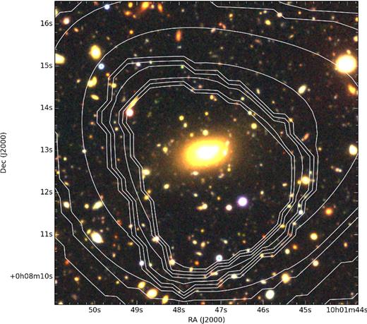
The X-ray emission contours overlaid on the optical RGB image of a galaxy group at z = 0.322 in the COSMOS field. The BGG is located in the X-ray centre of the hosting group.
Furthermore, we visually inspect all the BGGs in the optical red giant branch (RGB) image of hosting haloes (e.g. Fig. 2).
2.3 Stellar mass of the BGGs
The stellar mass and SFR are computed using le phare code (Arnouts et al. 2002; Ilbert et al. 2006). To start with, the redshift of BGG is fixed to the redshift of the hosting group. Then, similar to Ilbert et al. (2010), SED templates of galaxies generated by Bruzual & Charlot (2003) are fitted to the photometric measurements in u, g, r, i, and z bands using a χ2 minimization method. For consistency between data of different fields, we apply the same method as Ilbert et al. (2010) applied for the COSMOS sample.
The SED templates are generated assuming 0.02 and 0.008 metallicities, corresponding to 1 Z⊙ and 0.4 Z⊙, respectively, and exponentially declining SFR ∼ ∝e−t/τ where t is the age of a galaxy and τ have nine values between 0.1 and 30 Gyr. The Calzetti et al. (2000) extinction law is applied to the SEDs with six E(B − V) values of 0.0, 0.1, 0.2, 0.3, 0.4, and 0.5. Similar to Ilbert et al. (2010), Fontana et al. (2006), and Pozzetti et al. (2007), we force the prior E(B − V) < 0.15 if age/τ > 4 (a high extinction value is only allowed for galaxies with a high SFR).
In order to estimate the uncertainties in computing the stellar mass, we take into account the following sources of errors: (1) uncertainties in redshift determination, (2) lack of near-infrared bands; (3) photometric errors, and (4) an intrinsic error caused by SED fitting method. For the first source of error, similar to Ilbert et al. (2010), we compute the stellar mass for a galaxy sample with spectroscopic redshifts. Then we repeat the procedure by fixing their redshift to the one obtained photometrically. To measure the error in stellar mass induced by redshift uncertainty, we compare the stellar mass estimated using spectroscopic versus photometric redshifts. Since the photometric redshift error depends on photometric accuracy (generally brighter galaxies have more precise photometric redshift), the error induced by this uncertainty is also a function of galaxy luminosity. The error due to the lack of the near-infrared bands and photometric errors is derived by comparing the results of the stellar mass in the CFHTLS deep fields (in overlap with wide fields and with additional J, H, and K bands). This uncertainty is characterized as a function of the magnitude and redshift of galaxies. Similar to Giodini et al. (2012), we assumed 0.14 dex error induced by SED fitting method. In order to derive the total errors in the stellar mass estimation for XMM–LSS galaxies, we assume no correlation between aforementioned errors and thus add them in quadrature. Details of error analysis are presented in Mirkazemi et al. (in preparation).
For the BGGs in the COSMOS field, we use the information on the properties of galaxies provided by Ilbert et al. (2013), Capak et al. (2007), and McCracken et al. (2012). We note that the stellar mass and SFR of galaxies in the AEGIS field have been estimated using fast code (Kriek et al. 2009, which has been taken from Wuyts et al. 2011).
3 EVOLUTION OF THE STELLAR MASS
3.1 Distribution of the stellar mass of the BGGs
There are statistical studies of abundance matching, stacked lensing analysis, and clustering of galaxies that determine the mean occupation as a function of galaxy mass. These studies cannot probe the distribution of galaxy properties, e.g. stellar mass of galaxies for a given halo mass. The main advantage of our study is in the direct detection of galaxy groups which provides a unique opportunity to study the diversity of the BGG properties for a well-defined sample in terms of the mass and the redshift of objects.
Four, out of five, subsamples (S-II to S-V) of galaxy groups cover a similar halo mass range. These groups are rich galaxy groups and allow us to follow the evolutionary properties of their BGGs: the stellar mass distribution and the mass growth of the BGGs since z = 1.3 to z = 0.1. For each subsample, we construct the stellar mass distribution and quantify, in details, the shape of this distribution with respect to the normal distribution by fitting a single Gaussian distribution and measuring the skewness and the Kurtosis. We compare the best-fitting Gaussian parameter, namely the centre of the peak (Mcen), its height and the Gaussian width (σ), between the observations and SAMs predictions. We also quantify the stellar mass bin, MGd (Gd: Gaussian deviate), where the maximum deviation (e.g. secondary peak) is occurred between the observed stellar mass distribution and the best-fitting Gaussian distribution. The results are summarized in Table 1.
The best-fitting Gaussian distribution's parameters.
| Sample ID | Peak value | Peak centroid (log(Mcen/M⊙)) | Gaussian width (σ) |
|---|---|---|---|
| S-I: | |||
| Obs | 0.24 ± 0.02 | 10.9 ± 0.01 | 0.35 ± 0.01 |
| G11 | 0.19 ± 0.01 | 10.94 ± 0.01 | 0.19 ± 0.01 |
| DLB07 | 0.21 ± 0.01 | 11.01 ± 0.01 | 0.18 ± 0.01 |
| B06 | 0.11 ± 0.01 | 10.71 ± 0.01 | 0.32 ± 0.01 |
| S-II: | |||
| Obs | 0.18 ± 0.03 | 11.10 ± 0.03 | 0.33 ± 0.03 |
| G11 | 0.20 ± 0.01 | 11.17 ± 0.01 | 0.18 ± 0.01 |
| DLB07 | 0.22 ± 0.01 | 11.25 ± 0.01 | 0.16 ± 0.01 |
| B06 | 0.12 ± 0.01 | 10.97 ± 0.01 | 0.260 ± 0.01 |
| S-III: | |||
| Obs | 0.20 ± 0.02 | 11.25 ± 0.03 | 0.27 ± 0.03 |
| G11 | 0.22 ± 0.01 | 11.14 ± 0.01 | 0.17 ± 0.01 |
| DLB07 | 0.21 ± 0.02 | 11.18 ± 0.01 | 0.19 ± 0.01 |
| B06 | 0.13 ± 0.01 | 10.98 ± 0.01 | 0.32 ± 0.03 |
| S-IV: | |||
| Obs | 0.26 ± 0.02 | 11.15 ± 0.02 | 0.37 ± 0.02 |
| G11 | 0.20 ± 0.01 | 11.10 ± 0.01 | 0.21 ± 0.01 |
| DLB07 | 0.20 ± 0.01 | 11.14 ± 0.01 | 0.21 ± 0.01 |
| B06 | 0.13 ± 0.01 | 10.88 ± 0.01 | 0.30 ± 0.01 |
| S-V: | |||
| Obs | 0.25 ± 0.03 | 11.02 ± 0.02 | 0.35 ± 0.04 |
| G11 | 0.27 ± 0.01 | 11.05 ± 0.01 | 0.20 ± 0.01 |
| DLB07 | 0.31 ± 0.02 | 11.09 ± 0.01 | 0.19 ± 0.01 |
| B06 | 0.19 ± 0.01 | 10.76 ± 0.01 | 0.27 ± 0.01 |
In Fig. 3, we show the stellar mass distribution and the best-fitting Gaussian function to the observed data of BGGs (solid black histogram and curve) and that of the SAM of G11 (dotted red histogram and curve), DLB07 (dashed green histogram and curve), and B06 (dash–dotted blue histogram and curve), respectively.
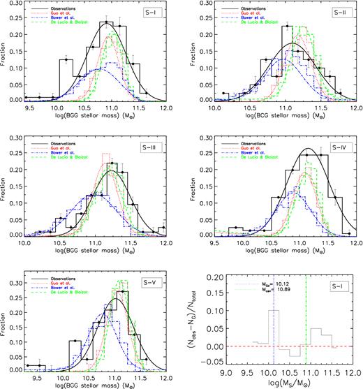
The stellar mass distribution of the BGGs and Gaussian approximations are shown as solid black histogram and curve, respectively. The predictions from the SAMs of G11, B06, and DLB07 are shown as the dotted red, dash–dotted blue, and dashed green histograms and curves, respectively. The lower-right panel shows the residual between the observed and the fitted fraction of the BGGs in similar stellar mass bins for S-I, the blue dotted and green dash-dotted lines correspond to the position of the maximum deviation (<log(MGd) >) of the observed distribution from the Gaussian distribution and the position of the centre of the peak in the Gaussian distribution (log(Mcen)).
The main findings are as follows.
(I) The subsample S-V shows a secondary peak at log(MGd/M⊙) ≈ 10.2. This peak is also seen in subsample S-III and S-II, however, the peak is slightly shifted towards higher mass bins. These galaxies with log(MGd/M⊙) ≈ 10.5 are a young population of BGGs. In a separate study we investigate the stellar age and SFR of this population.
(II) The subsample S-I also shows a strong deviation from the single Gaussian fit as there appears to be a secondary peak at the low-mass end. The peak is located in log(MGd/M⊙) ≈ 10.2. We note that this subsample covers a lower halo mass compared to other subsamples. We show the difference between the fraction of BGGs in the observed distribution (Nobs) and the best-fitting Gaussian distribution (NG) in each stellar mass bin for S-I in the lower-right panel in Fig. 3. The appearance of this secondary peak can also be suggestive of a newly forming BGGs.
(III) The observed distribution of the stellar mass covers a wide range. This appears to be only recovered by the B06 model which shows a similar Gaussian dispersion to the observational distribution of the stellar mass.
(IV) With a given similar stellar mass binsize, the peak value of stellar mass distribution is overpredicted by G11 and DLB07 in all subsamples.
(V) The location of the peak centroid is successfully reproduced by the G11 and the DLB07.
We find that both G11 and DLB07 models perform similarly in predicting the stellar mass distribution of the BGGs at all redshift and halo masses considered. However, the G11 prediction is closer to observations than the DLB07 model. This model is an updated and modified version of the SAM which was presented in DLB07, and both models share a number of prescription for the physical processes which were used in their implementations. However, the comparison between our findings in observations and the G11 predictions indicates that this model still needs further development.
Moreover, the discrepancies between observations and the three SAMs in particular at low masses can possibly be linked to the star-forming (SF) activities and the mass assembly history of the BGGs. For example, SAMs generally overestimate the number of the low-mass satellite galaxies, thus BGGs in models can possibly experience more minor mergers than the BGGs in observations. Recently, Cousin et al. (2015), constructed four SAMs, which three of them are classical SAMs and the 4th SAM is a model which is constructed based on a ΛCDM model with a correct number of the low-mass haloes and adopting two-phases gaseous disc: the first with the SF gas and the second with no-SF gas. They showed that even when a strong SN-feedback and photoionization are applied on the implementation of three classical SAMs, these models again form too many stars and overpredict the low-mass end of the stellar mass function. However, the 4th SAM is matched to the observations very well. They argue that at any given redshift, only a fraction of the total gas in a galaxy is used for the star formation activity.
3.2 Evolution of the shape of the stellar mass distribution
In Section 3.1, we find a secondary peak in the stellar mass distribution at low-mass tail, a feature that are not predicted by SAMs. The observed Gaussian parameters also seem to vary with redshift. In order to quantify the redshift evolution of the shape of the stellar mass distribution, we measure the Kurtosis and skewness values of the stellar mass distribution in each subsample as presented in Tables 2 and 3.
The kurtosis parameter of the stellar mass distribution of the BGGs in observations and SAMs, which are determined with respect to the normal distribution.
| Subsample ID | mean z | observations | G11 | DLB07 | B06 |
|---|---|---|---|---|---|
| S-I | 0.22 | −0.12 ± 0.53 | 0.02 ± 0.15 | −0.19 ± 0.15 | 1.00 ± 0.08 |
| S-II | 0.25 | −0.07 ± 0.63 | −0.34 ± 0.22 | −0.05 ± 0.24 | 0.05 ± 0.17 |
| S-III | 0.55 | 1.11 ± 0.56 | 0.63 ± 0.20 | −0.20 ± 0.20 | 0.20 ± 0.12 |
| S-IV | 0.84 | 1.69 ± 0.46 | 0.07 ± 0.20 | −0.01 ± 0.14 | 0.19 ± 0.12 |
| S-V | 1.15 | 1.74 ± 0.67 | 0.48 ±0.25 | −0.25 ± 0.26 | 0.08 ± 0.20 |
The skewness value of the stellar mass distribution of the BGGs in observations and SAMs which are computed with the normal distribution.
| Subsample ID | mean z | observations | G11 | DLB07 | B06 |
|---|---|---|---|---|---|
| S-I | 0.22 | −0.64 ± 0.27 | −0.37 ± 0.07 | −0.18 ± 0.07 | −0.64 ± 0.04 |
| S-II | 0.25 | −0.35 ± 0.32 | −0.31 ± 0.12 | −0.11 ± 0.12 | −0.58 ± 0.09 |
| S-III | 0.55 | −0.77 ± 0.26 | −0.28 ± 0.09 | −0.28 ± 0.10 | −0.58 ± 0.06 |
| S-IV | 0.84 | −1.07 ± 0.23 | −0.31 ± 0.10 | −0.40 ± 0.07 | −0.55 ± 0.06 |
| S-V | 1.15 | −1.24 ± 0.34 | −0.44 ± 0.13 | −0.15 ± 0.13 | −0.53 ± 0.10 |
The upper and middle panels of Fig. 4 shows the Kurtosis and skewness values of the stellar mass distribution of the BGGs versus the mean redshift of each subsample and linear fit. The observed trend is shown with the solid black line and the predicted trends have been shown with dotted red line (G11), dashed green line (DLB07), and dot–dashed blue line (B06), respectively. The non-connected symbols present results for S-I. The skewness of the stellar mass distribution tends to decrease with redshift. The negative values of this parameter indicates that the stellar mass distribution tends to skew more towards low masses. The Kurtosis value considerably increases with redshift indicating that the stellar mass distribution becomes progressively peaked. The predicted Kurtosis and skewness values by SAMs shows no or a little evolution. The B06 model has a best consistency with the data below z ∼ 0.5, but above this redshift all models fail to predict the observed stellar mass distribution of the BGGs.
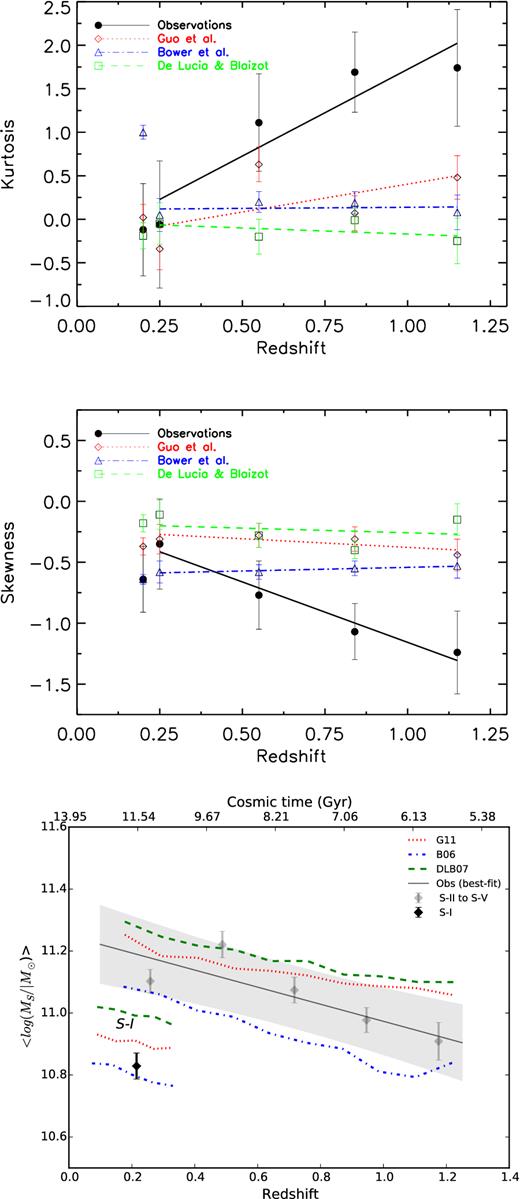
The Kurtosis of the stellar mass distribution of the BGGs versus redshift (upper panel). The skewness of the stellar mass distribution of the BGGs versus redshift (middle panel). The observed trend (solid black line) for the Kurtosis and skewness suggest that the shape of the stellar mass distribution evolves towards the normal distribution with decreasing redshift. The mean stellar mass of the BGGs versus redshift (lower panel). The grey highlighted area represents the 68 per cent confidence interval of the best fit to the data. The mean stellar mass of BGGs grows by a factor of ∼2 since z = 1.3 to present day.
Fig. 4 clearly demonstrates that the shape of the stellar mass distribution in observations significantly evolves towards a normal distribution with decreasing redshift. The shape of the stellar mass distribution in model predictions shows no evolution and this distribution approximately follows a normal distribution at all redshifts.
3.3 Evolution of the mean stellar mass of BGGs
The lower panel of Fig. 4 shows the evolution of the mean stellar mass of the BGGs in observations (filled dimonds) over the redshift range of 0.1 < z < 1.3. To quantify the growth of the mean mass of BGGs we re-sample BGGs within massive haloes (M200 = 1013.5 to 1014 M⊙) into 5 redshift bins. This helps to model the mean mass evolution more accurately. The solid grey line and the highlighted area indicate the best-fitting linear relation (< log(MS) > = (−0.27 ± 0.1)z + (11.24 ± 0.08)) to the observed data and its (68 per cent) confidence intervals, respectively. Using the best-fitting function, we find that the mean stellar mass of BGGs grows gradually by a factor of ∼2.07 since z = 1.3 to z = 0.1.
On the lowest panel of Fig. 4, we also show the evolution of the mean stellar mass of BGGs in the SAM predictions (G11, DLB07, and B06). The modelled trends are approximated by the best-fitting linear relations as follows (since models predict roughly linear trends, thus we ignore to plot these relations):
B06 : 〈log(MS)〉 = (−0.28 ± 0.02)z + (11.13 ± 0.02)
DLB07 : 〈log(MS)〉 = (−0.18 ± 0.01)z + (11.3 ± 0.01)
G11 : 〈log(MS)〉 = (−0.17 ± 0.01)z + (11.25 ± 0.01).
The mean stellar mass of BGGs in the SAM evolves by a factor of 2.09 (B06), 1.63 (DLB07), and 1.55 (G11) since z = 1.3 to z = 0.1, respectively. Evolution of the mean stellar mass of BGGs in all models is consistent with that of observations within the errors. Among models, the rate of stellar mass evolution in B06 is the closest to observations.
We note that there is some tension between model predictions and observations at z < 0.4, as the modelled slope of the stellar mass growth is steeper than that in the observations. In addition, the observed growth of the BGG mass mainly occurs at 0.4 < z < 1.3. Within observational errors, our findings are consistent with that of early studies e.g. Lidman et al. (2012) and Shankar et al. (2015). However, Lidman et al. (2012) have studied the brightest cluster galaxies assemblies within massive haloes and found that these object can grow in mass by a factor of 1.8 ± 0.3 at 0.1 < z < 0.9. In addition, the lack of the mass growth at low redshifts (z < 0.5) has also been argued by Oliva-Altamirano et al. (2014) and Lin et al. (2013).
In lower panel in Fig. 4, we separately show the mean mass of the BGGs in observations (filled black diamond) and models for S-I. DLB07 overpredicts the mean stellar mass of the BGGs for S-I, while B06 and G11 agree with observations.
3.4 The stellar mass and halo mass relation
We study the correlation between the stellar mass of the BGGs and the total mass (M200) of their host groups in observations and SAMs. We show the results in Fig. 5. The median value of the stellar mass of BGGs with the associated error (median absolute deviation) in each halo mass bin is also presented in this figure. Furthermore, we apply a robust linear regression and estimate the best-fitting relation (log(MS) = β × log(M200) + α) over the whole data in both observations and SAMs, presented in Table 4.
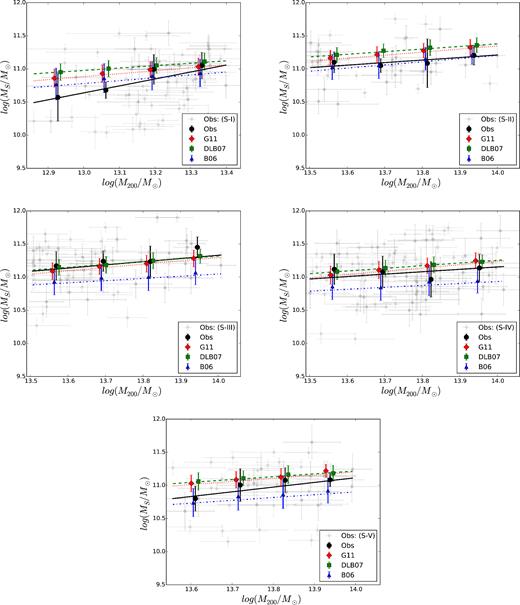
The stellar mass of BGGs against the group mass (M200) in observations (grey points) for S-I (top-left panel), S-II (top-right panel), S-III (middle-left panel) and S-IV (middle-right panel), and S-V (bottom panel), respectively. The dark circles and line, red diamonds and dotted line, green squares and dashed line, and blue triangles and dash–dotted line show the median trends and the best-fitting relation in observations and the SAMs of G11, DLB07, and B06, respectively. In agreement with model predictions the BGG mass is positively correlates with the host group mass.
The best-fitting relation (log(MS) = β × log(M200) + α) on the stellar mass and halo mass plane in observations and SAMs.
| Subsamples | β | α |
|---|---|---|
| S-I: | ||
| Obs | 1.05 ± 0.3 | −3.01 ± 3.9 |
| G11 | 0.45 ± 0.02 | 5.08 ± 0.23 |
| B06 | 0.43 ± 0.03 | 5.18 ± 0.38 |
| DLB07 | 0.36 ± 0.02 | 6.26 ± 0.21 |
| S-II: | ||
| Obs | 0.38 ± 0.24 | 5.85 ± 3.26 |
| G11 | 0.46 ± 0.04 | 4.88 ± 0.56 |
| B06 | 0.47 ± 0.07 | 4.56 ± 0.92 |
| DLB07 | 0.39 ± 0.04 | 5.87 ± 0.52 |
| S-III: | ||
| Obs | 0.48 ± 0.21 | 4.56 ± 2.89 |
| G11 | 0.5 ± 0.02 | 4.3 ± 0.27 |
| B06 | 0.33 ± 0.03 | 6.4 ± 0.43 |
| DLB07 | 0.43 ± 0.02 | 5.35 ± 0.26 |
| S-IV: | ||
| Obs | 0.36 ± 0.23 | 6.06 ± 3.12 |
| G11 | 0.49 ± 0.03 | 4.36 ± 0.42 |
| B06 | 0.29 ± 0.05 | 6.87 ± 0.65 |
| DLB07 | 0.4 ± 0.03 | 5.63 ± 0.37 |
| S-V: | ||
| Obs | 0.71 ± 0.37 | 1.2 ± 5.11 |
| G11 | 0.48 ± 0.05 | 4.5 ± 0.72 |
| B06 | 0.43 ± 0.08 | 4.94 ± 1.15 |
| DLB07 | 0.43 ± 0.05 | 5.2 ± 0.66 |
Our major findings are as follows: in accordance with model predictions, the trends show that the stellar mass of BGGs positively correlates with their host group mass at all redshifts, indicating that the massive haloes host massive BGGs. The observed median trend of the MS–M200 relation is consistent with model predictions within errors in all subsamples. We point out that the best-fitting relation in observations for S-I is steeper than that of the model predictions and the observed trend for S-II. This indicates that the stellar mass of BGGs within low-mass groups correlates more strongly with the halo mass compared to that of BGGs within massive groups at similar redshift range (0.04 < z < 0.4).
We find that the observed best-fitting relations for high-z subsamples (S-II to S-V) are almost similar and consistent with model predictions within uncertainties.
Previous studies have also shown that the stellar mass of the BGGs positively correlates with the hosting halo masses. For example, Stott et al. (2010) have shown that the stellar mass of the BGGs within their sample of 20 massive clusters at 0.8 < z < 1.5 is correlated with cluster mass. Recently, Oliva-Altamirano et al. (2014) also examined the MS–M200 relationship for both centrally and non-centrally located BGGs selected from the Galaxy And Mass Assembly survey at z = 0.09–0.27 and found that for both subsamples the MS–M200 relation follows a power law (∼0.32 ± 0.2).
4 STAR FORMATION ACTIVITY
4.1 Distribution and evolution of the specific star formation rate
A number of previous studies have shown that BGGs are generally passive galaxies and a large fraction of these systems exhibiting AGN activity, radio emission and no significant star formation at z < 1. The newly formed stars in these galaxies contribute ∼1 per cent of the total stellar mass of galaxy at late epochs z < 2 (Kauffmann et al. 2003; Edwards et al. 2007; Bildfell et al. 2008; O'Dea et al. 2008, 2010; Liu, Mao & Meng 2012; Thom et al. 2012).
In this study, the SFR of the BGGs in the AEGIS filed has been estimated using the fast code (Kriek et al. 2009) taken from Wuyts et al. (2011) and the SFR of the BGGs in the COSMOS and XMM–LSS fields have been obtained based on SED fitting (Ilbert et al. 2010). Both G11 and DLB07 similarly assume stars from gas cooling in the disc according to the empirical relation taken from Kennicutt (1998). However, G11 model refined the SAM used in construction of DLB07 model and the new modifications of physical processes (e.g. the treatments of the gas cooling and disc size) in this model lead the SFR to evolve significantly smoother than that in DLB07, with less star formation activity driven from ‘starburst’ in the bulk of the galaxies. For further information on the SFR estimate in models we refer to Section 3 in G11.
We present the distribution of the specific star formation rate (sSFR) of the BGGs in Fig. 6 and find the following.
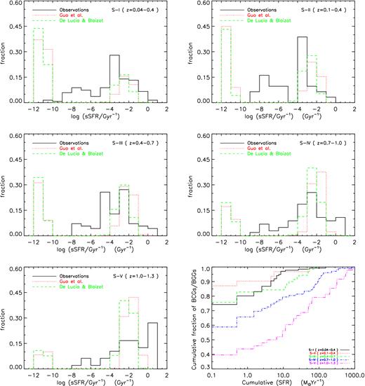
The sSFR distribution of the BGGs in observations and models(G11 and DLB07) for S-I (top-left), S-II (top-right), S-III (middle-left), S-IV (middle-right), and S-V(bottom-left). To adopt and illustrate the BGGs with SFR = 0, the SFR in both models and observations are shifted by dSFR = +1−9 M⊙ yr−1. (Bottom- right) The cumulative distribution of the SFR ( M⊙ yr−1) of BGGs in observations. We find that at least ∼20 ± 3 per cent of the BGGs are SF system with rates above >1 M⊙ yr−1.
For S-I, the log(sSFR/Gyr−1) spans a wide range between ∼−11 and 1 with a peak around log(sSFR/Gyr−1) ∼ −3 (top-left panel). A significant fraction (∼65 per cent) of BGGs in models show no star formation activity. The discontinuity in the computed values for the SFR in the SAM could well be a computational issue such that sSFR less than log(sSFR/Gyr−1) ≤ −4 is assumed to be insignificant. We note that the SFR of BGGs in models have been truncated at log(SFR/M⊙ yr−1) ∼ −3. With this in mind, about 40 per cent of the observed sSFR would be below the SAMs sensitivity to the SFR list of log(sSFR/Gyr−1) ≤ −4 compared to the ∼65 per cent in the models.
For S-II, the distribution of the BGG sSFR in observations is broadly similar to that of S-I and tends to skew towards low sSFR. In models, fraction of highly SF BGGs shows a slight increase relative to S-I (right-top panel).
For S-III, the distribution of the sSFR in observations indicates that the star formation has been significantly higher in the past. We find that fraction of the quiescent BGGs in models decreases by ∼15 per cent compared to the low-z BGGs (S-I and S-II) which follows the observed trend.
For S-IV and S-V, the sSFR distributions in observations and models further supports the increased star formation activities in BGGs at higher redshifts in both the observations and the models.
We find that the sSFR distribution tends to skew towards low sSFRs and also tends to peak less than a normal distribution at all redshifts. In addition, we mention that the sSFR distribution tends to skew more towards low sSFR with increasing redshift.
Further, we study the cumulative distribution of the SFR of BGGs in observations as shown in the bottom-right panel of Fig. 6. The vertical and horizontal axes represent the cumulative fraction of the BGGs and the cumulative SFR in each subsample, respectively. The gap between these cumulative distributions clearly shows that the fraction of SF BGGs increases with redshift. As a result, we find that ∼25 ± 5, 13 ± 2, 25 ± 5, 41 ± 7, and 60 ± 5 per cent of the BGGs within S-I to S-V have total SFR above 0.1 M⊙ yr−1 which can reach up to 1000 M⊙ yr−1. By comparing the cumulative distribution of SFR between S-I (solid black histogram) and S-II (dotted red histogram), it appears that BGGs within low-mass groups are more SF systems than the BGGs within massive groups in similar redshifts below z < 0.4.
4.2 Evolution of the average SFR of the BGGs
To further explore the SFR evolution with redshift, we compute the average SFR of all BGGs in each subsample and show against their mean redshift in Fig. 7. We find that the mean SFR of BGGs within rich groups (S-II to S-V) steeply declines from z = 1.3 to the present day, changing by roughly 1.98 dex M⊙ yr−1. This evolution is significantly stronger than the decrease in the SFR of galaxies as whole for a given mass by a factor of ∼30 from z ∼ 2 to z ∼ 0 (e.g. Daddi et al. 2007). The best-fitting relation to the evolution of the mean SFR of BGGs in observations with reshift is approximated as follows:
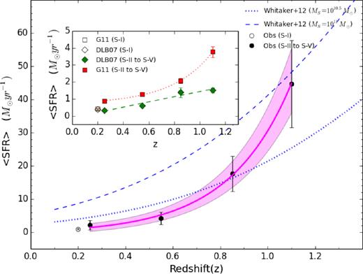
The redshift evolution of the average SFR of the BGGs in observations for S-I (black open circle) and for S-II to S-V (black filled circles). The magenta line and the highlighted area represent the best-fitting relation and its 68 per cent confidence intervals. The evolution in the SFR at two given masses (MS = 1010.5 and 1011 M⊙) in the SFR-mass sequence taken from Whitaker et al. (2012) have been shown with dotted and dashed lines, respectively. The average SFR of the BGGs in observations is less than the SFR of the MS galaxies with similar masses in the field and the BGG evolution is different from the MS evolution. The subplot shows the redshift evolution of the mean SFR of the BGGs in the G11 (red diamonds and line) and DLB07 (green squares and line) models, respectively.
〈SFR〉 = (0.70 ± 0.06)e(3.79 ± 0.10)z + (−0.39 ± 0.97).
The highlighted magenta area in Fig. 7 corresponds to the 68 per cent confidence intervals.
A systematic difference is seen between observations and model predictions, as explained in last section, thus we separately illustrate the SFR evolution with redshift for SAMs in Fig. 7. The best-fitting relation to the mean SFR-z plane in the G11 model also follows an exponential trend (〈SFR〉 = (0.098 ± 0.001)e(3.13 ± 0.1)z + (−0.68 ± 0.01)). In contrast, the DLB07 predicts a linear evolution for the SFR of BGGs with redshift (〈SFR〉 = (1.53 ± 0.28)z + (−0.10 ± 0.21)). The mean SFR of the BGGs for S-I is shown with open symbols in both observations and models predictions.
In addition, to compare the evolution of the average SFR of the BGGs with the evolution in the SFR of the SF galaxies, we use the SFR-stellar mass sequences (main sequence, MS) driven using a sample of 28 701 galaxies selected from the NEWFIRM Medium-Band Survey (NMBS; Whitaker et al. 2011) in a wide redshift range (0 < z < 2.5) as presented in Whitaker et al. (2012). Since the majority of the BGGs in observations have a masses around log(MS/M⊙) ∼ 11, We use function (1) in Whitaker et al. (2012) and determine the SFR evolution at log(MS/M⊙) = 11. In addition, we also estimate this evolution in the SFR-mass sequence (Whitaker et al. 2012) at log(MS/M⊙) = 10.5.
As a result, by comparing the evolution of the MS at log(MS/M⊙) ∼ 11 (dashed blue line) and the evolution of the average SFR of BGGs (solid magenta line), we find that the average SFR of BGGs is less than the SFR of the SF galaxies in the field in similar stellar masses. This indicates that the BGG evolution is different from the MS evolution.
4.3 Correlation between SFR and stellar mass
Fig. 8 highlights the relation between the SFR and the stellar mass of the BGGs. The observed data is overlaid on the same from the SAM of G11 (red diamonds) and DLB07 (green squares). For clarity, the BGGs with photometric redshift (black symbols) are distinguished from those with spectroscopic redshift (magenta symbols). We illustrate the SFR-stellar mass relation for the low-z subsamples (S-I (circles) and S-II (triangles)), the intermediate-z subsamples (S-III (circles) and S-IV (triangles)), and the high-z subsample (S-V) from top to bottom panels, respectively.
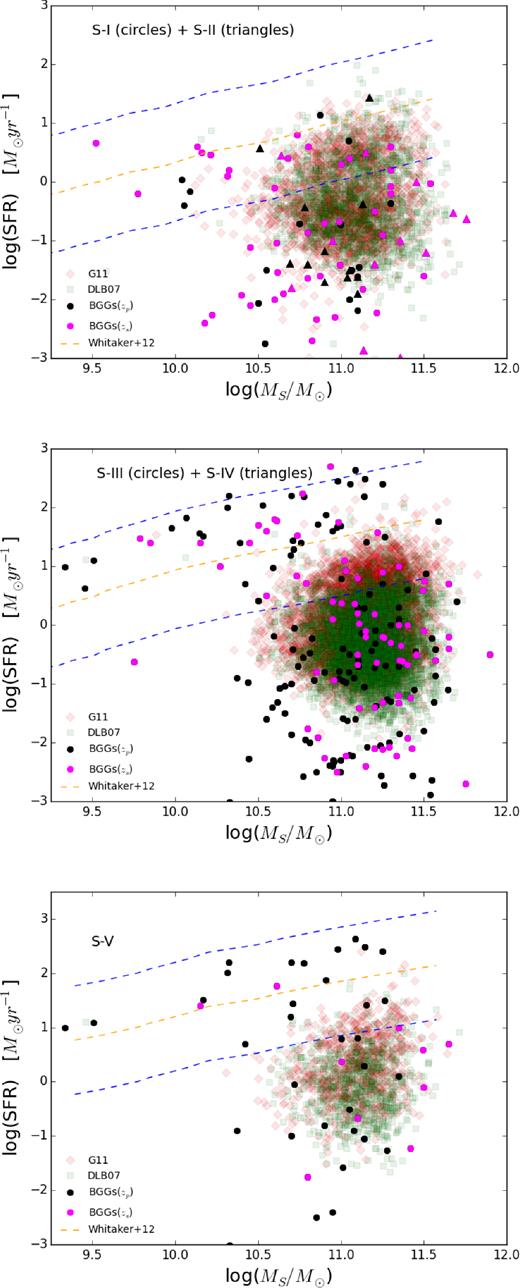
The BGG SFR versus their stellar mass for observations (black and magenta symbols) overlying on that from the SAM of G11 (red diamonds) and DLB07 (green squares). The magenta and black colours distinguish the BGGs with spectroscopic and photometric redshifts, respectively. Upper to lower panels present the SFR–MS plane for S-I+ S-II, S-III+ S-IV, and S-V, receptively. The dashed orange line represents the SFR mass sequence taken from Whitaker et al. (2012). The blue dashed lines represent ±1 dex M⊙ yr−1 limits from the SFR mass sequence. We select BGGs as a SF galaxy if its SFR lies on the SFR mass sequence between two dashed blue lines, if the BGG SFR falls below the lower level of this sequence it is classified as a passive galaxy.
We use the SFR-stellar mass sequences (Whitaker et al. 2012) to define SF, starburst and passive BGGs in our sample (e.g. Elbaz et al. 2007; Erfanianfar et al. 2014). Galaxies spend most of their life on the MS and keep their SF activity as normal SF systems. As their star formation activities are quenched, they fall below the MS and become as passive/quiescent galaxies. In contrast, as a galaxy experiences a merger or becomes in the close encounter with another galaxy, it may undergo an exceptionally high rate of star formation it moves above the MS and spend a short fraction of its life in this region. In this phase, this galaxy is identified as a starburst galaxy. The dashed orange line in Fig. 8 represents the position of the SFR-mass sequences at 0.0 < z < 0.5 (upper panel), 0.5 < z < 1.0 (middle panel), and 1.0 < z < 1.5 (lower panel) taken from Whitaker et al. (2012).
Therefore, we define a BGG as a SF galaxy if it falls on the MS, i.e. between the two dashed blue lines which correspond to ±1 dex M⊙ yr−1. We define a BGG as passive galaxy, if the SFR of this galaxy falls below the lower limit (−1 dex) from MS for a given stellar mass.
In Fig. 8, we find that the fraction of galaxies falling in the SF region increases with redshift in observations, while the trend is less clear in the models. We also find that the majority of the low-mass BGGs (log(MS/M⊙) < 10.5) lie within the SFR-mass sequences. We also find that galaxies with stellar mass of log(MS/M⊙) = 10.5–11 exhibit a bimodal distribution between the low- and high-mass galaxies.
In addition, the sSFR–MS plane for S-III to S-IV (middle panel) shows the presence of some highly SF, starburst, BGGs in observations close to(or above) the star formation MS.
A considerable number of the BGGs, in models, show no star formation activity and they fall out of the SFR range which is adopted in Fig. 8. Thus to have a better comparison between observations and model predictions we bin stellar mass of BGGs and compute the number of passive and SF BGGs in each bin. The number of passive/SF BGGs in each stellar mass bin is normalized to the total number of the BGGs in each subsample. The left-hand and right-hand panels of Fig. 9 show the fraction of SF BGGs (fSF) and the fraction of passive BGGs (fpas) as a function of their stellar mass, respectively. In upper and middle panels in Fig. 9, we present results for the combined data of S-I+S-II and S-III+S-IV, respectively, since the trends for these combined subsamples were similar. As a result, for all subsamples, we find that the fraction of SF BGGs decreases with increasing stellar mass with a corresponding increase of passive BGGs. The passive fraction at fixed stellar mass seems to increase at lower redshift. Interestingly, G11 shows an increasing fraction of SF with mass in contrast to the observation. The DLB07 prediction agrees better than G11 with observations at z < 1. The trends in observations and models show no significant dependence to redshift.
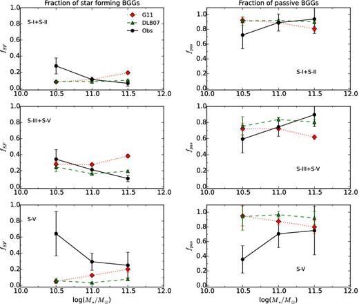
The fraction of the SF (fSF) (left-hand panels) and the passive (fpas) (right-hand panels) BGGs versus the stellar mass of BGGs for S-I+S-II, S-III+S-IV, and S-V. The solid black line, dotted red line, dashed green line illustrate the trends in observations and the G11 and DLB07 models, respectively.
Although we do not explicitly show in the paper, we find a similar trend, as seen in Fig. 9, in the fraction of SF and passive BGGs as a function of the halo mass for both models and observations.
4.4 Specific star formation rate versus redshift and M200
Finally we study the evolution of the sSFR and its relation with the halo mass. Fig. 10 shows the redshift dependence of the median sSFR for S-I (left-hand panel) and for S-II to S-V (right-hand panel), respectively. The error bars in data points corresponds to the median absolute deviation in each redshift bin. In agreement with model predictions, the sSFR of BGGs for S-I show no significant change with redshift. In Fig. 10, we also probe the log(sSFR)–z relation in the SAMs. Models predict a flat trend over z < 0.4. The left-hand panel in Fig. 10 shows that on the other hand, in S-II to S-V, the sSFR of BGGs increases mildly with increasing redshift between z = 0.1 to z = 0.7. SAMs predict a slow evolution over 0.1 < z < 1.3 which they may marginally agree with observations within errors.

In Fig. 11, we show the median sSFR dependence of BGGs to the total mass of their host groups in observations (black points) and in the SAMs of G11 (red diamonds) and DLB07 (green squares), respectively. For S-I (left-hand panel), the median sSFR rapidly decreases as a function of increasing halo mass (the best-fitting linear relations corresponds to: SFR/Ms = (−4.4 ± 1.0) × M200 + (3.8 ± 0.8). The observed trend is steeper than the model predictions. In agreement with the SAM predictions, we find no relationship between sSFR and M200 for S-II to S-V over 0.1 < z < 1.3, as shown in the right-hand panel in Fig. 11. These results suggest that, in the group scale haloes, sSFR of BGGs is a function of redshift with no halo mass dependence.
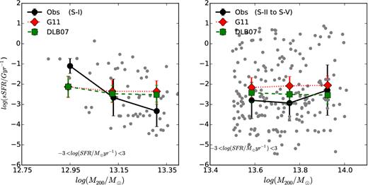
The SFR/Ms–M200 relation for S-I (left-hand panel), and for S-II to S-V (right-hand panel). The solid, dashed, and dotted lines show the median trends for BGGs in observations and in the SAM of DLB07 and G11, respectively. The grey point shows the BGG sSFR versus redshift in observations. Only, for BGGs within S-I we find that the sSFR decreases as a function of halo mass.
5 SUMMARY AND CONCLUSIONS
We select the BGGs in a well-defined X-ray-selected sample of galaxy groups from the COSMOS, XMM–LSS, and AEGIS fields. This sample covers a redshift range of 0.04 < z < 1.3 and contains about 407 galaxy groups with a mass ranging from 1012.8 to 1014 M⊙, the largest sample for such studies in the X-ray galaxy group regime. The sample allows us to study the distribution and evolution of the stellar mass and SFR of BGGs and the relation among the stellar mass, SFR, and halo mass. We compare our results with sample drawn from the Millennium simulations with three SAMs (G11, DLB07, and B06). We summarize our results as follows.
The shape of the stellar mass distribution of the BGGs evolves towards a normal distribution as the groups evolve. This evolution is quantified by the skewness and Kurtosis of the stellar mass distribution and their redshift dependence. At all redshifts, we find that the stellar mass distribution tends to skew towards low masses. The observed fraction of the BGGs shows a strong deviation from the Gaussian fit at ≈1010.2 M⊙, which are generally SF/young population. In contrast, the SAM predictions show no redshift evolution of the stellar mass distribution. Within the probed SAMs, the shape of the stellar mass distribution predicted by B06 model is more consistent with the observations at z < 0.5.
We show that the average stellar mass of the BGGs evolves with redshift by a factor of ∼2 from z = 1.3 to the present day. At z < 0.4, the mean stellar mass shows no significant evolution and the significant growth of BGGs occurs at 0.4 < z < 1.3. The observed evolution is broadly consistent with the prediction of the ΛCDM model, and previous studies (e.g. Lidman et al. 2012; Lin et al. 2013; Oliva-Altamirano et al. 2014). Furthermore, the SAMs of G11, DLB07, and B06 predict that BGGs grow in stellar mass by a factor of 1.55, 1.63, and 2.09, respectively. The rate of the mean stellar mass evolution with redshift in B06 prediction has the best agreement with observations.
We find that the BGG stellar mass increases with the halo mass, with a weak redshift dependence. In addition, the stellar mass of BGGs within low-mass groups (S-I) correlates more strongly with host halo mass compared to that of BGGs within massive haloes at similar redshift range (z < 0.4).
We show that the BGGs are not completely inactive or quenched systems as their SFR can reach ∼1000 M⊙yr−1. At least ∼13 ± 3 to 60 ± 5 per cent of BGGs in our low-z (S-II) and high-z (S-V) subsamples are galaxies with SF rate above ∼1 M⊙yr−1. We indicate that the average SFR of BGGs steeply increases with redshift in particular at z > 0.7. The best fit to the data in observations is as follows: 〈SFR〉 = (0.70 ± 0.06)e(3.79 ± 0.10)z + (−0.39 ± 0.97). We compare the evolution of the average SFR of BGGs with the evolution in the SFR of the SF galaxies (MS) using the SFR-mass sequence presented in Whitaker et al. (2012). We find that evolution of the average SFR of BGGs is different from the evolution of MS. In addition, the SAMs underestimate the average SFR of BGGs in observations in similar stellar masses.
We find that the fraction of SF BGGs decreases with increasing stellar mass with a corresponding increase of passive BGGs. In addition, the passive fraction at fixed stellar mass seems to increase at lower redshift. Interestingly, G11 shows an increasing fraction of SF with mass in contrast to the observation, while fraction of the passive BGGs increases with increasing stellar mass. The DLB07 prediction agrees better than G11 with observations at z < 1. We note that the relation between fraction of the SF/passive BGGs and the total mass of groups is similar to that is seen between these fractions and the stellar mass of BGGs.
For BGGs in massive groups (S-II to S-V), we find that sSFR slightly increases with increasing redshift at z < 0.7, and above this redshift, the trend of the sSFR evolution becomes steep. While the sSFR of BGGs for S-I shows no significant change with redshift. We also find that the sSFR of BGGs within low-mass groups (S-I) decreases with increasing halo mass. However, in agreement with model predictions, the sSFR of BGGs within massive groups (S-II to S-V) shows no dependence to the halo mass.
We have been able to probe semi-analytic galaxy formation models, publicly available, using the observations of the stellar mass, SFR and their halo dependencies. We demonstrate and argue that these observations are highly useful for constraining the models.
This work has been supported by the grant of Finnish Academy of Science to the University of Helsinki, decision number 266918. The first author wishes to thank School of Astronomy, Institute for Research in Fundamental Sciences for their support of this research. MM acknowledges the support by the DFG Cluster of Excellence ‘Origin and Structure of the Universe’ and the Computational Center for Particle and Astrophysics (C2PAP), located at the Leibniz Supercomputer Center (LRZ). We used the data of the Millennium simulation and the web application providing online access to them were constructed as the activities of the German Astrophysics Virtual Observatory.
REFERENCES
