


Abstract
We report the flux measurement of the Vela-like pulsar B1800−21 at the low radio frequency regime over multiple epochs spanning several years. The spectrum shows a turnover around the GHz frequency range and represents a typical example of gigahertz-peaked spectrum (GPS) pulsar. Our observations revealed that the pulsar spectrum show a significant evolution during the observing period with the low-frequency part of the spectrum becoming steeper, with a higher turnover frequency, for a period of several years before reverting back to the initial shape during the latest measurements. The spectral change over times spanning several years requires dense structures, with free electron densities around 1000–20 000 cm−3 and physical dimensions ∼220 au, in the interstellar medium (ISM) traversing across the pulsar line of sight. We look into the possible sites of such structures in the ISM and likely mechanisms particularly the thermal free–free absorption as possible explanations for the change.
1 INTRODUCTION
The pulsar radio emission is non-thermal in nature and characterized by a steep power-law spectra. Generally, the observed spectra can be modelled with a negative spectral index of about −1.8 in the frequency regime between 0.1 and 10 GHz (Maron et al. 2000). The gigahertz-peaked spectrum (GPS) observed in a handful of cases, where a turnover is seen in the spectra around 1 GHz (Kijak, Gupta & Krzeszowski 2007), provide a deviation from the general pulsar population. These sources are mostly present in exotic environments with associated dense H ii regions or Pulsar Wind Nebulae (PWNe). The GPS nature is believed to originate due to interaction of the pulsar emission with the surrounding medium but is still poorly understood. In order to discover more cases of GPS pulsars and gain better understanding of this peculiar phenomenon, systematic studies have been carried out over the past few years (Kijak et al. 2011a,b, 2013; Dembska et al. 2014, 2015a,b).
The majority of GPS pulsars are characterized by high dispersion measure (DM > 200 pc cm−3), which may very well be a coincidence of the specialized environments that harbour them. The conventional flux measurement techniques which rely on estimating the baseline level of the pulse profile may be affected by interstellar scattering which results in smearing of the pulse across the entire period. In some cases, when the pulse broadening time is a significant fraction of the pulse period (30 per cent or more) one can see a relatively sharp pulse, but at the same time the extended scattering tail may obscure the real baseline level, which leads to an underestimation of the pulsar flux. For pulsars with DMs in 200–300 pc cm−3 range this usually happens between 300 and 600 MHz (Lewandowski et al. 2013, 2015a). This leads to a somewhat pseudo-correlation between high DM and GPS pulsars (Kijak et al. 2007, 2011b) where serious underestimation of the flux at lower frequencies for high DM pulsars may give rise to an inverted spectra. The interferometric imaging technique provide a more robust measurement of the pulsar flux owing to the baseline lying at zero level thereby reducing errors made during the baseline subtraction. Dembska et al. (2015b), D15 hereafter, used the imaging technique to measure the flux of six high DM pulsars at 610 MHz to explore their suspected GPS nature. Their studies revealed that in four of the six cases the measured flux was underestimated due to scattering effects and the corrected flux followed a normal power-law spectra. In pulsar B1823−13 they confirmed the presence of GPS characteristics. However, the case of PSR B1800−21 defied expectations as the interferometric flux measurements turned out to be significantly lower than the earlier measurements using conventional methods. This gave rise to various questions regarding the spectral nature of this pulsar. There was also a possibility of the two measurement techniques being incompatible and errors during the measurement processes.
In this work, we carry out a detailed study of the spectrum in PSR B1800−21 spanning multiple frequencies and different epochs. Interferometric flux measurements at 325 and 610 MHz at two widely separated epochs were carried out. In addition, a complete low-frequency spectrum for the pulsar was constructed by using data at 325, 610 and 1280 MHz, separated over short intervals, simultaneously with a phased array and an interferometer. In each of these cases, the radio spectra of PSR B1800−21 were constructed and revealed GPS characteristics. PSR B1800−21 is a young pulsar similar to the well-known Vela pulsar and is associated with a very interesting environment. The pulsar lies within the W30 complex which comprises of a supernova remnant (SNR) and a number of compact H ii regions (Kassim & Weiler 1990; Finley & Oegelman 1994). This makes the pulsar a well-suited candidate for exhibiting GPS characteristics. We carry out a detailed comparison of our measured spectra with previously reported values (Lorimer et al. 1995; Kijak et al. 2011b; D15) and look into the possible implications.
2 OBSERVATIONS AND DATA ANALYSIS
We used the Giant Metrewave Radio Telescope (GMRT) for our studies which is an interferometric array consisting of 30 dishes in a Y-shaped array spread out over a region of ∼27 km. The GMRT is uniquely positioned to be used simultaneously as an interferometer and a phased array due to alternate routes of signal post-processing for these two modes. We carried out observations which enabled us to compare the flux measurements using the two different techniques and verify previous flux values. The GMRT operates in the metre wavelengths at five distinct frequency bands around 1.4 GHz, 610, 325, 240 and 150 MHz with a bandwidth of 33 MHz at each frequency spread over 256 frequency channels. For our studies, we have used the three frequencies 1280, 610 and 325 MHz during one or more epochs to measure the flux in pulsar B1800−21. The lower frequencies were not used for our studies as the pulsar was expected to have an inverted spectrum and the flux values would be below detection limit at these frequencies. The observations were carried out over three different epochs between 2013 December and 2015 September as detailed in Table 1. Each of the observations were carried out for more than an hour and at each epoch the pulsar was observed twice separated by at least a week to account for variations due to scintillation.
Observing details for PSR B1800−21.
| Obs date | Frequency | Obs mode | Calibrator | Cal flux |
|---|---|---|---|---|
| (MHz) | (Jy) | |||
| 2013 Dec 28 | 610 | Int | 1822−096 | 6.2 ± 0.4 |
| 2014 Jan 07 | 610 | Int | 1822−096 | 6.2 ± 0.4 |
| 2015 Jan 03 | 325 | Int | 1822−096 | 2.7 ± 0.2 |
| 2015 Jan 17 | 325 | Int | 1822−096 | 3.4 ± 0.3 |
| 2015 Aug 15 | 610 | Int/Ph | 1714−252 | 4.7 ± 0.3 |
| 2015 Aug 20 | 325 | Int/Ph | 1822−096 | 3.3 ± 0.3 |
| 2015 Aug 23 | 1280 | Int/Ph | 1751−253 | 1.0 ± 0.1 |
| 2015 Aug 29 | 610 | Int/Ph | 1714−252 | 4.5 ± 0.3 |
| 2015 Sep 03 | 1280 | Int/Ph | 1714−252 | 2.4 ± 0.2 |
| 2015 Sep 14 | 325 | Int/Ph | 1714−252 | 5.0 ± 0.3 |
Notes. Int–Interferometric; Ph–Phased array.
We used standard observing schemes where the flux calibrator 3C286 was recorded at the start of each observing run and strategically placed phase calibrators (see Table 1) interspersed at regular intervals. The Astronomical Image Processing System (aips) was used for imaging as detailed in D15. The flux scale of the calibrator 3C286 was set using the latest Perley-Butler (2013) estimates (in aips) and was used to calculate the flux of the different phase calibrators as shown in Table 1. In the phased array mode, the signal from each of the antennas (around 20 nearby antennas were used) were co-added to produce a time series data with resolution 122 μs. The antennas were phase aligned at regular intervals on the phase calibrator before being co-added for maximum signal-to-noise measurements. The data were dedispersed and a folded profile for each observation was obtained using the topocentric pulsar period (Fig. 1). We used publicly available softwares tempo1 and the ATNF pulsar data base2 (Manchester et al. 2005) for determining the different parameters of the pulsar B1800−21 during our observing runs. All the calibrators were observed in the on–off mode, where data were recorded with the antennas pointing away from the source before recording on the source. The resulting shift in the count level from the background gave a scaling factor for the measured counts to the flux levels in jansky. The average pulsar flux from the pulse profiles were calculated after subtracting the baseline and suitably scaling with the scaling factor. Finally, the average flux during all the epochs for each observing frequency were determined for the two observing modes and shown in Table 2.
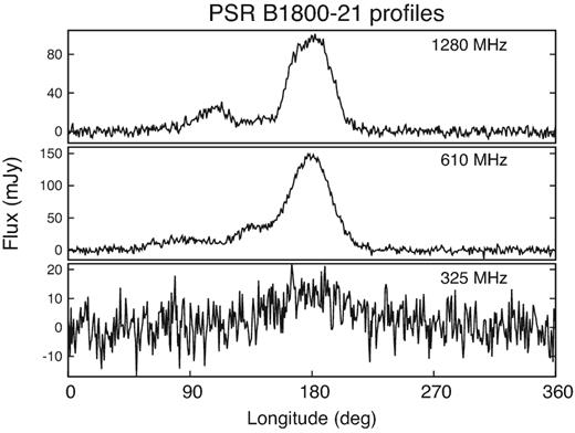
Profile of the pulsar B1800−21 measured using GMRT at the three radio frequencies 1280, 610 and 325 MHz. The observations were carried out between 2015 August and September. The pulsar flux decreases considerably at the lowest frequency where the profile also exhibits scattering.
Flux measurement for PSR B1800−21.
| Observation date | Frequency | Intfr flux | Ph-Arr flux |
|---|---|---|---|
| (MHz) | (mJy) | (mJy) | |
| 2013 Dec–2014 Jan | 610 | 9.2 ± 0.7 | – |
| 2015 Jan | 325 | 3.4 ± 0.3 | – |
| 2015 Aug–2015 Sep | 325 | 3.4 ± 0.2 | 2.2 ± 2.6 |
| 2015 Aug–2015 Sep | 610 | 12.8 ± 0.9 | 14.3 ± 4.8 |
| 2015 Aug–2015 Sep | 1280 | 13.9 ± 1.0 | 12.8 ± 3.5 |
3 RESULTS
3.1 Interferometer versus phased array
One of the primary goals of our studies was to verify the compatibility of the two different techniques used to measure the pulsar flux. This was prompted by the results reported in D15 where the measured flux of B1800−21 using interferometric method was considerably lower than the previously reported measurements at 610 MHz (Kijak et al. 2011b). We have carried out simultaneous flux measurements using the two techniques at three different frequencies as shown in Table 2. The measurements are identical at all the three frequencies, within measurement errors, showing the two methods to be mutually consistent in determining the flux of pulsars. It is still possible that one or more of the reported flux in the literature is affected by observing errors, but our studies confirm that there is no measurement bias due to the observing technique employed. We look into the implications of the spectral nature of the pulsar B1800−21 with emphasis on the physical conditions in the following sections. It is worth noting that Table 2 shows the interferometric flux measurements to be more accurate with smaller errors compared to the phased array values. This may be due to a number of reasons which we list below.
(1) In the phased array the number of antennas used (∼20) is less than the antennas used for the interferometric measurements (≧ 27). This is because in the phased array mode the signals from each antenna is phase aligned at regular intervals on a calibrator before being co-added for higher signal-to-noise detection. The further apart the antennas are the faster the alignment is lost and as a result only nearby antennas are used to save time on phasing. The interferometer on the other hand records all the correlation between antenna pairs where the phase alignment is done offline. This requires longer computation time during analysis but all the available antennas can be used for the measurements.
(2) The interferometer records the correlation between two antennas as a result of which the baseline due to background is at zero level. This results in more robust measurements free from the errors made during baseline subtraction while estimating the scaling factor and pulsar profile in the phased array. A significant drawback of the phased array flux measurement arises in the case of highly scattered pulsars with long tails rendering baseline levels indeterminate. The interferometric measurements provide the only secure way of estimating flux in these sources (see D15).
(3) Finally, the most important advantage using the interferometer is that the instrumental and atmospheric gain fluctuations can be corrected on very short time-scales using self-calibration of the interferometric data. These corrections are determined by flux densities of constant and bright background sources in the field and considerably reduces the noise levels.
The number of data points recorded at any instant is considerably larger in an interferometer compared to a phased array. Hence, the time resolution of an interferometer is significantly lower which is a major drawback in conventional pulsar studies. However, this is not a primary requirement for flux estimation where the interferometric technique provides a superior alternative to other traditional means.
3.2 Spectral nature of PSR B1800−21
The observations reported in this paper were spread out over a period of about two years and were motivated by the significantly lower flux measurements of the pulsar B1800−21 reported in D15, observed on 2012 December, compared to the previous epochs. Our measurements between 2013 December and 2014 January at 610 MHz were consistent with the flux values reported in D15 within measurement errors, though the actual values in 2013–2014 (9.2 ± 0.9 mJy, Table 2) were slightly higher than in 2012 values (7.4 ± 0.9 mJy in D15). The low-frequency flux from 2015 January onwards have been much higher and closer to the earlier reports. We believe that our results in conjunction with D15 show an evolution of the low-frequency spectrum of the pulsar B1800−21 in recent times where the low-frequency part of the spectrum became steeper around 2012–2014 which has once again reverted to the original shape (as in 2009 and earlier) in 2015. In Fig. 2, the pulsar spectra is shown at three different epochs, before 2009 using archival measurements, between 2012 and 2014 and finally from 2015 January 2015. In all three cases the spectra exhibit GPS characteristics. The thermal free–free absorption in the intervening medium first proposed by Kijak et al. (2011a, 2013) to explain GPS behaviour and further extended by Lewandowski et al. (2015b) has been utilized to model the spectrum in each case with the spectral fits and errors during fitting shown as solid and broken lines, respectively, the details of which are presented in the next section. The GPS behaviour is characterized by the turnover in the pulsar radio spectra around the GHz frequency range. The turnover frequency is seen to change from 0.80 GHz before 2009 to 1.05 GHz between 2012 and 2014 which changed to 0.77 GHz in 2015. Though there have been studies reporting the change in the pulsar period, DM, etc. at short time-scales, we believe our results are the first such reported case of spectral change taking place within time-scales of several years.
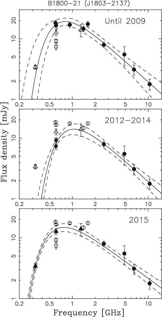
The radio spectra for the pulsar B1800−21 measured during different observing epochs. The circular points represent the flux values from the literature measured before 2009, the square points show the measurements during the period between 2012 December and 2014 January. The measurements carried out after 2015 January are shown as triangular points. The solid line represents the fitted model during each epoch of observation and the dashed lines correspond to the 1σ envelope for all possible fits (the fitting procedure is described in the main text). For each case, the spectral fits were performed only using the measurements denoted by filled symbols with the empty symbol measurements shown only for comparison. All three spectral fits included the high-frequency data (2 GHz and above) from before 2009, to help us constrain the intrinsic pulsar spectrum (since at these frequencies the effects of thermal absorption should be negligible). The GPS characteristic is visible during each epoch of observation.
3.3 The fitting procedure
The parameters obtained by modelling of the spectrum of PSR B1800−21 for three different epochs (see also Fig. 2).
| Obs epoch | A | B | α | χ2 |
|---|---|---|---|---|
| (mJy) | (K−1.35 pc cm−6) | |||
| Until 2009 | |$1.94^{+0.76}_{-0.70}$| | |$0.34^{+0.18}_{-0.17}$| | |$-1.12^{+0.24}_{-0.28}$| | 1.33 |
| 2012–2014 | |$1.93^{+0.46}_{-0.45}$| | |$0.59^{+0.17}_{-0.17}$| | |$-1.12^{+0.22}_{-0.25}$| | 0.81 |
| 2015 | |$2.16^{+0.44}_{-0.41}$| | |$0.258^{+0.035}_{-0.035}$| | |$-0.93^{+0.12}_{-0.12}$| | 0.73 |
3.4 Interpretation of spectral changes
In this section, we analyse the constraints on the physical parameters of the absorber based on our modelling and the measured value of the dispersion measure (DM = 233.99 ± 0.05 pc cm−3; see Hobbs et al. 2004).
(i) dense filaments in SNR with typical s = 0.1 pc,
(ii) cometary shaped tail in PWN with s = 1.0 pc,
(iii) and H ii region with s = 10.0 pc.
As a first step towards understanding the turnover in the spectra, we used the initial spectra (before 2009) and for each of the above three configuration of the absorber determined the physical parameters (the temperature and electron density) required for explaining the B parameter reported in Table 3 (first line). The physical parameters for each of the three categories are shown in Table 4, titled ‘Initial absorber’.
The constraints on the physical parameters of the absorbing medium for both the initial and additional absorption (see text for detailed explanation).
| s | ne | T | |
|---|---|---|---|
| (pc) | (cm−3) | (K) | |
| Initial absorber | |||
| 0.1 | 1170 | 2200 | |
| 1.0 | 117 | 400 | |
| 10.0 | 12 | 73 | |
| Additional absorber | |||
| 0.001 | 16 657 | 5000 | |
| 0.001 | 3520 | 500 | |
| 0.001 | 1188 | 100 |
| s | ne | T | |
|---|---|---|---|
| (pc) | (cm−3) | (K) | |
| Initial absorber | |||
| 0.1 | 1170 | 2200 | |
| 1.0 | 117 | 400 | |
| 10.0 | 12 | 73 | |
| Additional absorber | |||
| 0.001 | 16 657 | 5000 | |
| 0.001 | 3520 | 500 | |
| 0.001 | 1188 | 100 |
One of the main outcomes of our studies have been the discovery of the change in the pulsar spectra (see Fig. 2) between 2012 and 2014. The absorption during this period was much stronger as evidenced by the higher value of the B parameter in Table 3. We suggest that this excess absorption was caused by an additional absorber that moved across the line of sight. In this scenario, the overall optical depth is a sum of the contributions from the initial absorber and the additional component. Using equations (2) and (3) along with the difference between the values of B parameter estimated for the initial (until 2009) and the increased absorption period (between 2012 and 2014), we can constrain the physical parameters of this additional absorber. The size of the additional absorber can be estimated using the pulsar's transverse velocity and the duration over which the spectral change was seen. Our observations were inadequate to determine the actual time-scales for the spectral change; however, the minimum and maximum duration was five years and one year, respectively. We used a mean duration of three years for the change and |$v = 347^{+57}_{-48}$| km s−1 (Brisken et al. 2006) to estimate the physical size of the additional absorber to be s ∼ 0.001 pc (approximately 220 au). We assumed that the physical dimensions of the additional absorber were identical along the transverse direction and the line of sight. We lack any measurement of the DM during the period between 2012 and 2014 which once again presented a degenerate problem with both the temperature and electron density of the additional absorber being unknown. We have once again considered three situations where such conditions can arise in the ISM and assumed the typical temperatures as shown in Table 4, lower part titled ‘Additional absorber’. The required electron densities for each case is calculated and shown in the table.
In the next section, we explore the consequence of our estimates of the physical parameters of the absorber on the pulsar emission and particularly their environmental implications.
4 DISCUSSION
The pulsar B1800−21 is young (age ∼ 16 kyr) with a high spin-down energy loss (Ė = 2.2 × 1036 erg s−1) and is similar to the well-known Vela pulsar which also shows a turnover in the spectrum around 600 MHz (Sieber 1973). PSR B1800−21 has a very distinct environment and is believed to be associated with the W30 complex (Kassim & Weiler 1990; Finley & Oegelman 1994). The W30 complex is a roughly spherical structure consisting of SNR G8.7−0.1 and a large number of compact H ii regions in and around it. The pulsar is located in the south-west direction near the edge of the SNR. Detailed proper motion studies by Brisken et al. (2006) have ruled out a direct association between PSR B1800−21 and the SNR, with the pulsar moving approximately towards the centre of the SNR. High-resolution X-ray analysis using the Chandra X-Ray observatory have revealed the pulsar to be associated with a compact PWN (Kargaltsev, Pavlov & Garmire 2007). We do not have a detailed estimate of the conditions in the immediate vicinity of the pulsar which makes it difficult to constrain the spectral fitting. However, we used information about the different structures seen around the pulsar to constrain the physical properties of the absorber responsible for the GPS phenomenon as shown in Table 4. The proximity of the pulsar with the SNR is the motivation for invoking the filamentary structures seen in SNRs as a likely source for the observed GPS phenomenon (Kijak et al. 2011b), the first condition in Table 4 (Initial absorber, ne = 1170 cm−3, T = 2200 K). The physical parameters of the filament required for the observed turnover in the spectrum (around 800 MHz) is similar to the measured values in certain cases (Koo et al. 2007). It is noteworthy that given the small size of the filaments, it is rare for these structures to be moving across the line of sight of a pulsar. The second condition in Table 4 (Initial absorber, ne = 117 cm−3, T = 400 K) corresponds to the GPS phenomenon associated with an asymmetric PWN as has been detected around PSR B1800−21 (Kargaltsev et al. 2007). The GPS phenomenon driven by bow-shock nebula has been investigated by Lewandowski et al. (2015b) where the phenomenon is affected by the relative orientation of the direction of pulsar emission and the shape of the bow shock. The physical parameters in such a situation is consistent with our estimates. In principle, we do not know how an asymmetric PWN will affect the pulsar spectrum, but we cannot exclude the possibility of GPS phenomenon arising in these systems. Finally, the presence of H ii regions near the pulsar prompted us to investigate the third condition in Table 4 (Initial absorber, ne = 12 cm−3, T = 73 K). It should be noted that several of the H ii regions around the PSR B1800−21 show a turnover in the spectrum near the GHz frequency range which can be attributed to thermal absorption (Kassim & Weiler 1990). It is possible to have large H ii regions with electron densities around 10–100 cm−3 but the temperatures associated with them are much higher (1000–10 000 K; Tsamis et al. 2003), which is contrary to our expectations for the observed GPS phenomenon. Thus, we discount these parameters as the physical characteristics of a potential absorber. The above discussions highlight that the likely condition giving rise to the GPS phenomenon in this pulsar is the absorption in filamentary structures in the surrounding SNR which may also account for the changes seen in the pulsar spectrum, as discussed below. However, we cannot completely discount the possibility of the detected PWN affecting the pulsar spectrum.
The most remarkable feature about PSR B1800−21 was the variation of the low-frequency spectrum within a time-scale of few years. The pulsar spectrum has steepened resulting in the turnover frequency shifting from 800 MHz to 1.05 GHz which changed back to its old shape after a period of few years. The pulsar radio emission mechanism is a highly tuned phenomenon (Melikidze, Gil & Pataraya 2000; Gil, Lyubarsky & Melikidze 2004) and it is difficult to envision a scenario where such a spectral change can occur without fundamentally altering the emission itself. The more likely possibility is the change in the intervening medium either in the vicinity of the pulsar or along the line of sight to the source. The shifting of the spectrum towards higher frequencies implies an increase in the relative absorption by the medium requiring the pulsar emission to pass through a more dense region. If we take into account the pulsar transverse velocity, the structures which will likely give rise to the change in the spectrum would be of size ∼220 au, for the changes to happen over roughly three years time span. We have used the distance to the pulsar to calculate the size of the absorber which will decrease if the absorber is located nearer. It was much more difficult to constrain the physical parameters of the absorber capable of causing such events without any obvious physical structures to guide us. We selected three temperature ranges between 100 and 5000 K to find out the electron densities of the absorber needed to explain the observed change in turnover frequency. The electron densities were much higher between 1000 and 20 000 cm−3 as shown in Table 4 (Additional absorber). As mentioned earlier, these are extreme physical conditions in the ISM which justifies the rarity of such detections. One likely absorber of interest is the ultracompact H ii regions which are believed to be small photoionized nebulae produced by O and B stars inside the clouds of molecular gas and dust in the ISM. These objects are characterized by electron densities >10 000 cm−3 and temperature around 1000–10 000 K and are extremely compact in size <0.1 pc (Wood & Churchwell 1989). Another possible candidate for such absorbers are the dense filaments seen in SNRs. There have been reported compact structures with electron densities >1000−3 and temperatures >1000 K in the Crab nebulae (Sankrit et al. 1998). However, it should be noted that the Crab nebulae is a special case and it would be difficult to find such structures in a standard SNR. In the remainder of this section, we discuss two events observed in pulsars where changes in pulsar emission over short time-scales (months to years) have resulted due to possible structures in the ISM.
In light of the discussions carried out above an astrophysical phenomenon that deserves particular attention is the extreme scattering events (ESEs) in the ISM. The ESEs are believed to originate due to dense structures in the ISM with sizes of the order of au causing extreme scattering and flux absorption when light from background sources pass through them. The ESEs are known to span time-scales ranging from a few weeks to several years and were first detected in flux of compact extragalactic sources such as quasars (Fiedler et al. 1987). These events are pretty rare and particularly harder to detect as they require constant surveillance of the flux over periods of several years. In subsequent years, ESEs have also been seen along the line of sight of some pulsars where the events are characterized by the decrease in the pulsar flux and increase in the DM lasting months to years before reverting back to the original values (Lestrade, Rickett & Cognard 1998; Maitia, Lestrade & Cognard 2003; Coles et al. 2015). It is to be noted that the few cases where multifrequency data are available the flux reduction at lower frequencies is greater than that at higher frequencies during the ESEs which is a signature of thermal absorption. The structures giving rise to ESEs are ideally suited to account for the change in the pulsar spectra over the time-scales of years with estimated physical sizes in au scales and densities ∼1000 cm−3. The observed change in the spectrum of PSR B1800−21 over a period of few years between 2012 and 2014 is a possible ESE reflected in the spectrum of the pulsar.
Another event of interest in connection with change in pulsar flux is the phenomenon of echoes associated with the Crab pulsar (Backer, Wong & Valanju 2000; Graham Smith & Lyne 2000). An echo was seen following the pulsed emission in the pulsar profile and was believed to be a result of scattering by ionized clouds far away from the pulsar along the line of sight and contained within the Crab nebula. This was associated with a reduction in the pulsar flux and increase in the DM lasting several hundred days. Observations were carried out at two different frequencies, 327 and 610 MHz, and it is clear that the change in the flux was more at the lower frequency (Backer et al. 2000), which is once again a signature of thermal absorption. A number of models have been proposed involving refraction and lensing effect by a plasma lens along the line of sight (Graham Smith, Lyne & Jordan 2011) with varying degree of success. The filamentary structures in the outer parts of the Crab nebula with physical dimensions of ∼ au and electron densities 1000 cm−3 are proposed as the most likely cause of such events. The rarity of these events also highlights the paucity of such structures around a nebula. In a direct extension to our studies, the filamentary structures are the ideal candidates to account for the spectral changes seen in PSR B1800−21 via thermal absorption if they happen to be along the line of sight. The presence of a surrounding SNR provides further ground for the likelihood of such rare structures around the pulsar.
To summarize our results, we have carried out detailed observations of the pulsar B1800−21 at the low-radio frequency regime with the objective of determining the spectrum. We used two different measurement techniques, the phased array and interferometer, and demonstrated the equivalence of these methods in estimating the pulsar flux. We confirmed the pulsar spectrum to exhibit GPS characteristics (Kijak et al. 2011b; D15). We reported the first instance of a change in the spectrum within a period of years with the turnover frequency shifting to a higher value before regaining its old form. This is most likely due to thermal absorption in compact dense structures along the line of sight. We have carried out a detailed statistical fit to the spectrum of the pulsar during all the epochs of observation and using basic assumptions about three structures in the ISM, filaments in SNR, PWN and H ii regions, determined the physical parameters responsible for the GPS phenomenon. Based on the physical arguments we found the H ii region to be an unlikely candidate as the absorber. The physical conditions in the ISM likely to give rise to the detected shift in the turnover frequency was more difficult to constrain. We investigated phenomenon such as ESEs and echoes in the Crab pulsar where compact structures responsible for short-term change in pulsar radio emission are possible candidates for the spectral change in PSR B1800−21. The detection of the GPS phenomenon in pulsars provides another possibility of probing their environments. These objects are usually found around interesting environments such as PWNe and SNRs and provide additional evidence of association between pulsars and these specialized surroundings. The number of pulsars showing GPS phenomenon is still very small and we lack information about the physical constituents of these environments to distinguish between the absorption at different stages of the SNR as well as the PWN. The discovery and characterization of the GPS phenomenon in a wider sample of pulsars would provide important insights into the physical compositions and the evolution of their environments.
This work was supported by grants DEC-2012/05/B/ST9/03924 and DEC-2013/09/B/ST9/02177. We thank the anonymous referee for useful comments. We thank the staff of the GMRT who have made these observations possible. The GMRT is run by the National Centre for Radio Astrophysics of the Tata Institute of Fundamental Research.
REFERENCES
