


Abstract
We present the results from a study of the morphologies of moderate luminosity X-ray-selected active galactic nuclei (AGN) host galaxies in comparison to a carefully mass-matched control sample at 0.5 < z < 3 in the CANDELS GOODS-S field. We apply a multiwavelength morphological decomposition analysis to these two samples and report on the differences between the morphologies as fitted from single Sérsic and multiple Sérsic models, and models which include an additional nuclear point-source component. Thus, we are able to compare the widely adopted single Sérsic fits from previous studies to the results from a full morphological decomposition, and address the issue of how biased the inferred properties of AGN hosts are by a potential nuclear contribution from the AGN itself. We find that the AGN hosts are indistinguishable from the general galaxy population except that beyond z ≃ 1.5 they have significantly higher bulge fractions. Even including nuclear sources in our modelling, the probability of this result arising by chance is ∼1 × 10⁻⁵, alleviating concerns that previous, purely single Sérsic, analyses of AGN hosts could have been spuriously biased towards higher bulge fractions. This data set also allows us to further probe the physical nature of these point-source components; we find no strong correlation between the point-source component and AGN activity. Our analysis of the bulge and disc fractions of these AGN hosts in comparison to a mass-matched control sample reveals a similar morphological evolutionary track for both the active and non-active populations, providing further evidence in favour of a model where AGN activity is triggered by secular processes.
1 INTRODUCTION
The physical processes responsible for triggering active galactic nuclei (AGN) are still uncertain. Despite the fact that many galaxy evolution models invoke major mergers to both trigger AGN and transform the underlying host galaxy morphologies from disc to bulge-dominated systems (e.g. Hopkins et al. 2005; Springel, Di Matteo & Hernquist 2005), there is mounting observational evidence that mergers may not play a dominant role and instead AGN activity may be driven by more secular processes (Gabor et al. 2009; Cisternas et al. 2011; Kocevski et al. 2012; Schawinski et al. 2012; Rosario et al. 2015).
If major mergers are the main mechanism for fuelling AGN activity, then the associated morphological changes of the host galaxies should provide clear evidence of this interaction. This evidence could manifest as a change from disc to bulge-dominated systems, or, if observed during the transformation period, to mixed bulge+disc systems exhibiting highly disturbed morphologies.
Locally, AGN hosts are indeed found to reside in more bulge-dominated systems (e.g. Kauffmann et al. 2003) and there are several well-known relations such as the strong correlation between black hole (BH) mass and bulge luminosity (e.g. Kormendy & Richstone 1995; Magorrian et al. 1998; Peng 2007; Jahnke & Macciò 2011) and the link between BH mass and stellar velocity dispersion (e.g. Ferrarese & Merritt 2000; Gebhardt et al. 2000) that suggest there is a strong connection between, and potentially co-evolution of, the central BH and the galactic bulge.
At higher redshifts (z ≥ 1), we also see evidence of AGN hosts displaying more bulge dominated, or mixed bulge+disc morphologies from high-resolution studies conducted with Advanced Camera for Surveys (ACS) on Hubble Space Telescope (HST). From comparing the hosts of X-ray-selected moderate luminosity AGN to a control sample, Grogin et al. (2005) showed through the use of non-parametric concentration measurements that the AGN hosts are more bulge dominated. Moreover, the study of Simmons & Urry (2008) has reported on the recoverability of the separation of point source and host galaxy light using single and multiple component parametric fits to simulated ACS data within this redshift regime.
However, there is also growing evidence within this higher redshift regime that AGN hosts do not display any excess of disturbed morphologies, another key signature of mergers, in comparison to control samples. Using both visual classifications and parametric fits of a sample of z ∼ 1 X-ray-selected AGN, Gabor et al. (2009) and Cisternas et al. (2011) observe that the host galaxies are no more disturbed than a control sample. Overall the AGN host morphologies in these studies do appear to be transitioning from disc to bulge dominated but as many of the AGN hosts retain discs, the authors conclude that the AGN activity in these systems has not been triggered by major mergers. In fact, Cisternas et al. (2011) note that the lack of morphological signatures of major mergers, in terms of disturbed structures, cannot simply be explained by a time lag between the merger event and the time at observation, because if these systems had undergone a merger prior to their epoch of observation one would not expect to find the AGN in such dynamically relaxed disc systems.
With the advent of high-resolution near-infrared (IR) imaging provided by WFC3/IR on HST, the CANDELS survey has allowed the rest-frame optical morphologies of AGN hosts in this redshift regime to be explored in more detail. Kocevski et al. (2012) and Rosario et al. (2015) confirm that while the majority of X-ray-selected AGN hosts at z ∼ 2 are discs, in comparison to a mass-matched non-active control sample, the AGN hosts have higher bulge fractions. However, these studies have been limited to single Sérsic morphological fits and/or visual classifications and so do not directly trace the different bulge and disc fractions within the two populations.
The study of Mechtley et al. (2015) has also utilized the WFC3/IR data to analyse the rest-frame optical host galaxy morphologies of a subset of quasars at z ∼ 2 and find no evidence for enhanced interaction signatures in the quasar sample compared to a non-active control sample.
Schawinski et al. (2012) extended the rest-frame optical analysis of AGN hosts to include a heavily obscured AGN sample. As simulations predict that major mergers will first trigger obscured AGN systems, which then become unobscured at later times, this analysis searched for morphological features of a merger in less evolved AGN systems. Schawinski et al. (2012) found no evidence for disturbed morphologies within this sample and concluded that the majority of heavily obscured AGN also resided in disc-dominated hosts (again using single Sérsic classifications, albeit with careful examination of residuals for additional structure), seeming to confirm the growing picture that AGN activity is not fuelled by mergers, but instead may be triggered by secular processes. However, see also Kocevski et al. (2015) for a similar study of spectroscopically identified Compton-thick AGN.
This observed trend for AGN hosts to exhibit disc-dominated morphologies, with larger contributions from a bulge component than matched control samples, makes it clear that both the bulge and disc components play an important role in the triggering of AGN. Further insight into this aspect of AGN evolution is given by Schramm & Silverman (2013) who decompose AGN host morphologies and compare the MBH–Mtotal and MBH–Mbulge relations at z ∼ 1 to their local counterparts. They find that, while the total stellar mass in the high-redshift AGN hosts is already in agreement with the local relation, there must be a transfer of mass from the disc to the bulge in order to build up the local MBH–Mbulge relation since z ∼ 1, in agreement with the previous findings of Jahnke et al. (2009) using HST/ACS and Near Infrared Camera and Multi-Object Spectrometer data. It is not clear that major mergers play the dominant role in this process and in fact secular processes such as violent disc instabilities (e.g. Dekel et al. 2009; Ceverino, Dekel & Bournaud 2010) or in fact minor mergers (van der Wel et al. 2014) may be key for such a transformation, as they are thought to be in the evolution of non-active massive galaxies within this redshift regime. These findings again lend support to a scenario for AGN hosts in which a viable explanation for their mixed bulge+disc morphologies and a self-consistent build up towards local relations is not (at least solely) dependent on major mergers.
In order to better explore the influence of both the bulge and disc components on the evolution of AGN, in this paper, we conduct a full multiwavelength decomposition of AGN hosts and a large mass-matched control sample into the separate bulge and disc components and test how the different morphological analyses often adopted in literature effect the best-fitting morphologies of the hosts. For the purposes of this work, we select a sample of moderate luminosity X-ray-selected AGN taken from the 4Ms Chandra data and identified as AGN on the basis of X-ray and multiwavelength analysis, and spectroscopic features where available (Xue et al. 2011). The increased depth of the 4Ms imaging results in more sensitivity to obscured AGN and is comparable to the maximum X-ray flux which can be attributed to star formation alone (Bauer et al. 2002). As a result, our sample contains a limited range of obscured AGN, in addition to some potential contamination at lower X-ray luminosities from starbursts.
This analysis utilizes the morphological decomposition technique presented in Bruce et al. (2012), which was extended to encompass full multi-wavelength decompositions in Bruce et al. (2014) and applied to samples in both the CANDELS Ultra Deep Survey and Cosmological Evolution Survey fields for M* > 1011 M⊙ galaxies at 1 < z < 3. For the purposes of this paper, we concentrate on the H160-band (F160W) morphological decompositions results, adopting light fractions for the individual components measured from the H160-band decompositions, and quoting decomposed stellar masses for the bulge and disc components based on the total stellar masses of the systems subdivided according to the light fractions for each component (as was shown in Bruce et al. 2014 to be representative of the fully decomposed SED fitted stellar masses).
This is the first work to self-consistently decompose the morphologies for a large sample of mass-matched control objects and AGN hosts at z > 0.5 and as such provides new insight into the directly measured bulge and disc fractions of the active and non-active populations. We also address how the adoption of a nuclear point source impacts the host fits, as there is some suggestion from previous studies that the more bulge-dominated morphologies fitted to AGN hosts may be biased by a contribution from the AGN itself.
From the alternative perspective, point-source fits are also adopted in non-active galaxy fits, often in single Sérsic fits which would otherwise exceed n = 10, and are deemed to be motivated by the presence of either an AGN or a nuclear starburst. Thus, this work provides the ideal data set with which to test the physical nature of the point-source components in addition to exploring how they impact the fits of known AGN.
This paper is structured as follows. In Section 2, we describe the data set used for this work, discuss the photometric redshift and stellar-mass fitting employed and present our mass-matching technique. Following this, in Section 3, we detail the morphology fitting techniques adopted. In Section 4, we present the results of our analysis for both the single and multiple component Sérsic models and discuss in detail the impact of the addition of point-source components on the fitted morphologies. In this section, we also briefly explore the connection between BH mass and both total and bulge stellar mass by investigating trends within our sample selection. Finally, in Section 5, we extend this discussion to the physical nature of these point-source components by exploring their trends with various observed properties. We conclude in Section 6 with a summary of our findings placed within the context of current models for AGN drivers and galaxy evolution as a whole.
Throughout we calculate all physical quantities assuming a Λcold dark matter universe with Ωm = 0.3, ΩΛ = 0.7 and H0 = 70 km s− 1 Mpc− 1.
2 DATA
For this work, we have used the HST WFC3/IR and accompanying multiwavelength data from the CANDELS multicycle treasury programme (Grogin et al. 2011; Koekemoer et al. 2011) in the GOODS-S field. The CANDELS GOODS-S field has been observed as part of the various tiers of the CANDELS observing strategy and so comprises CANDELS wide+deep+Early Release Science (ERS) imaging and covers a total area of ∼170 arcmin2 in the F160W and F125W filters, with the deep and wide fields covered in the F105W filter and the ERS field covered in the F098M filter. The corresponding 5σ point-source depths in the F160W filters are 27.6 (AB mag) in deep, 26.8 in wide and 27.3 in the ERS field. The CANDELS imaging in the GOODS-S field is accompanied by extensive existing multiwavelength data ranging from the X-ray to the mid-IR and UV. For the purposes of this work, we make use of the optical imaging from HST/ACS in the F435W, F606W, F775W and F850LP bands taken as part of the GOODS Hubble Treasury Programme (Giavalisco et al. 2004), and combine this with: U band from Visible MultiObject Spectrograph (VIMOS) (Nonino et al. 2009) and Cerro Tololo Inter-American Observatory (CTIO); Ks band from Infrared Spectrometer And Array Camera (Retzlaff et al. 2010); and Spitzer/IRAC 3.6-8 μm imaging from the GOODS Spitzer Legacy Programme (PI Dickinson) and spectral energy distributions (SEDs) (PI Fazio; Ashby et al. 2013).
In order to make use of the high-resolution HST/WFC3 and ACS imaging in combination with the low-resolution ground-based and confused mid-IR data, we adopt the GOODS-S CANDELS catalogue of Guo et al. (2013), which is generated from the co-added max-depth F160W GOODS-S mosaic for the deep+wide+ERS fields. In brief, the Guo et al. (2013) catalogue is constructed from an adapted version of sextractor (Galametz et al. 2013) run on hot and cold mode on the F160W mosaic and merged (Barden et al. 2012) to produce a detection catalogue, which is then used in sextractor dual mode on the point spread function (PSF) matched HST/WFC3 and ACS mosaics to provide a multiwavelength catalogue. The flux measurements for the objects in this catalogue are corrected to total based on an aperture correction determined in the F160W detection-band of fluxauto/fluxiso, for all but the smallest objects (isophotal radii < 2 pixels) for which the accuracy of the PSF matching becomes significant and for which the aperture correction is given by fluxauto/fluxaper,2pixels. The total fluxes from the lower resolution and confused data are then measured using the tfit code (Laidler et al. 2007) which is based on a template fitting approach. It is the Guo et al. (2013) photometry catalogue which has been used for photometric redshift fitting and which we use for stellar-mass fitting.
2.1 Photometric redshift and stellar-mass fitting
The photometric redshifts used in this work are taken from the Dahlen et al. (2013) GOODS-S CANDELS catalogue. The Dahlen et al. (2013) analysis explores the effects on redshift fitting from different codes, stellar population templates and the implementation of additional fitting procedures such as fitting emission lines, adopting photometric zero-point corrections from a spectroscopic training set and interpolating between templates. Dahlen et al. explore the redshift fits from 11 different groups and compare to a spectroscopic control sample of ∼600 galaxies. All of the fitting codes use the same photometric catalogue taken from Guo et al. (2013). The implemented catalogue contains 14 bands for each object: U-band VIMOS, F435W, F606W, F775W, F850LP HST/ACS, F098M or F105W, F125W, F160W HST/WFC3, Ks ISAAC, 3.6, 4.5, 5.8, 8 μm Spitzer/IRAC. Overall, they do not find that a specific code performs significantly better than the others but that the scatter in, and the outlier fraction of, the best-fitting photometric redshifts is best improved by combining the multiple fits, although the exact procedure for combining the results does not strongly influence the best fits. Here we use the best-fitting photometric redshifts from six of the fitting codes combined with a hierarchical Bayesian method (Lang & Hogg 2012).
We evaluate stellar masses using the best-fitting photometric redshifts from Dahlen et al. (2013). These masses have been estimated using the SED fitting code based on HYPERZ (Bolzonella, Miralles & Pelló 2000; Cirasuolo et al. 2007; Bruce et al. 2012) with a 12-band photometry catalogue taken from Guo et al. (2013): U band CTIO and VIMOS, F435W, F606W, F775W, F850LP HST/ACS, F098M (ERS field) or F105W (deep+wide fields), F125W, F160W HST/WFC3, Ks ISAAC, 3.6 and 4.5 μm Spitzer/IRAC. For the fitting, we adopt the Bruzual & Charlot (2003) models with single-component exponentially decaying star formation histories with e-folding times in the range 0.3 < τ(Gyr) < 5, with a minimum model age limit of 50 Myr and a Chabrier initial mass function. Absorption from the intergalactic medium is accounted for using the prescriptions of Madau (1995), and the Calzetti et al. (2000) obscuration law is used to account for reddening due to dust within the range 0 ≤ Av ≤ 4.
2.2 Sample selection
Given that the aim of this work is to explore the decomposed morphologies of AGN hosts within the context of a matched sample of non-active galaxies, we have utilized the Hsu et al. (2014) counterparts of the Xue et al. (2011) and Rangel et al. (2014) 4Ms Chandra catalogue to select moderate luminosity, LX > 1 × 1041 erg s−1, AGN from which we define a master sample of galaxies containing these AGN candidates (which have a median X-ray luminosity of 4.9 × 1042 erg s−1). In order to maximize the overlap between our samples (as discussed further in Section 4.4), we adopt a redshift range of 0.5 < z < 3 and a stellar mass threshold of M* > 1010 M⊙. Within this sample, 90 per cent of objects are ≳ 45σ detections in the H160 band, providing acceptable signal to noise for the morphological decompositions.
2.3 Mass and redshift matching
For a sample cut at M* > 1010 M⊙, the mass distribution for AGN host galaxies is centred towards higher masses than that of the control sample of galaxies (Rosario et al. 2013). As a result, in order to conduct a robust comparison between the physical properties of these two populations they must be matched in mass (within redshift bins of Δz = 0.5 to negate any differences in mass-redshift trends), so as not to introduce any biases. However, in order to fully exploit our much larger non-active galaxy sample (∼1600 objects), for each redshift bin, we create a 1000 times bootstrapped, mass-matched, control sample similar to the procedure adopted in Rosario et al. (2015), but crucially containing the maximal number of control objects as is allowed by the data whilst still ensuring that the mass distributions in the control and AGN host samples are consistent at the >95 per cent confidence level using a two sample Kolmogorov–Smirnov (K–S) test.
In this way, we ensure that the uncertainties in the comparison between the control sample and the AGN host sample are driven predominantly by the relatively low number of AGN hosts in each mass bin relative to the control sample. For all further analysis concerned with the comparison between AGN hosts and non-active galaxies, the distributions of physical properties of the control galaxy sample are given by the median of the 1000 bootstrapped samples within each bin for the different properties.
The mass and redshift distributions of our matched control sample and AGN hosts are shown in Fig. 1.
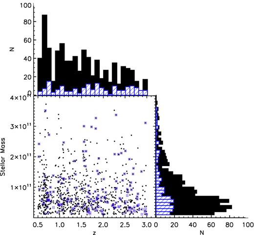
Mass and redshift distributions for the AGN host and mass-matched control samples. In the central panel, we show the two-dimensional distributions of the masses and redshifts for the X-ray-selected AGN host sample in blue and the maximally selected non-active, mass-matched control sample in black. In the top histogram, we display the redshift distributions for the control sample in black and the AGN hosts in blue, and likewise in the right histogram, we plot the stellar mass distributions for the two samples.
Finally, we perform some additional cross-checks with AGN selected in different ways. First, we compare to a sample selected based on the observed variability of their optical photometry by Falocco et al. (2015). Given the relatively small area of the CANDELS GOODS-S field there is only a small overlap between the samples, but we find that those selected from optical variability within our mass and redshift range were already included in the Hsu et al. (2014) catalogue. We also compare to a sample of Compton-thick AGN selected by Del Moro et al. (20165) and find another three AGN which are not in our original sample but are within our control sample and are fitted with pure disc morphologies. We conclude that by using an X-ray-selected AGN sample, we are selecting the largest fraction of radiatively luminous AGN and do not include the Compton-thick AGN in our analysis as our aim in this work is to explore any potential biases in the morphology fits of AGN hosts from a contribution from the AGN itself, and a Compton-thick sample should be the least affected by this. As a result, our conclusions apply to this subset of X-ray-selected AGN.
3 MORPHOLOGICAL ANALYSIS
For the morphological analysis presented in this paper, we implement the procedure developed by Bruce et al. (2012, 2014) using the two-dimensional light profile fitting code galfit (Peng et al. 2002, 2010). In brief, we conduct the morphological analysis in the WFC3 F160W H160 band, the reddest band available in the CANDELS survey which best represents the majority of the assembled stellar mass in the systems we are probing. The PSF we adopt is a hybrid composed of a TinyTim model (Krist 1995) in the central regions with an empirical fit used in the outskirts [for more details of the hybrid PSF generation, see van der Wel et al. (2012)]. We conduct two different classes of morphological fits: the first includes single Sérsic and single Sérsic + point-source components; and the second involves a full decomposition into the separate bulge, disc and point-source components. Throughout this analysis, we limit our fits to bulges with Sérsic indices locked at n = 4 (de Vaucouleurs bulges) and discs with Sérsic indices fixed to n = 1 (exponential profiles). We also fix the centroid of each component, and thus only allow the magnitude, effective radius, axial ratio and position angle of each component to be free parameters in the fitting. Background determinations are conducted externally from within fixed, blank apertures and are applied prior to the fitting with galfit. In order to decompose our objects appropriately, by default we adopt the simplest best-fitting model and only accept a more complex model where it is statistically motivated given a likelihood ratio analysis, similar to the Bayesian Information Criterion test (Schwartz 1978) adopted by other authors. In order to combat cases where the galfit χ2 minimization routine iterates towards local rather than global minima, we start each fit with multiple different initial conditions to better explore the χ2 parameter space for each fit.
For the purposes of this paper, we concentrate on only the H160-band morphological fits and defer a full description of the multiwavelength decompositions which allow us to conduct individual component SED fitting to analyse the physical nature of the point-source components to the companion paper (Bruce et al., in preparation), where we will discuss this in detail.
From our previous analysis and work with recovering simulated objects from within the CANDELS images (Bruce et al. 2014), we report uncertainties on bulge and disc magnitudes of ∼10 per cent, and size measurement of 10–20 per cent for discs and bulges, respectively. We have also explored the recoverability of point-source-affected objects and the prevalence of ‘false positive’ adoptions of these centrally concentrated compact models. We find that our procedure does not preferentially favour the adoption of a point-source component to deal with complex bulge+disc systems. Less than 0.5 per cent of bulge+disc fits of varying B/T light ratios and sizes ratios adopt a spurious point-source component when such a component is not included in the simulated object, and degeneracies between the point-source component and the bulge only become considerable when the simulated bulges are unresolved (with effective radii < 1 pixel). Thus, we conclude that the point-source components fitted in this analysis are robust and genuine morphological features.
4 MORPHOLOGICAL COMPARISON
As discussed in the introduction of this paper, detailed morphological AGN host galaxy studies are implicitly difficult due to the need for high-resolution deep imaging. Within the redshift range probed by this study, the CANDELS survey (Grogin et al. 2011; Koekemoer et al. 2011) has provided the ideal data set with which to conduct these types of studies. There are already several studies which address the morphological structure of moderate luminosity X-ray-selected AGN with this data set and as they provide an ideal basis against which to compare our newly decomposed morphologies, they are discussed briefly here for completeness. We note that the study of Schawinski et al. (2011) was the first work to utilize the WFC3 imaging on HST for AGN host galaxy analysis, but due to their smaller field coverage we do not directly compare to those results here.
The first of the studies we compare to is Kocevski et al. (2012) which is concerned with the visual classification of the near-IR morphologies of the host galaxies of the Xue et al. (2011) 4Ms Chandra X-ray-selected AGN in the ERS and deep regions of the CANDELS GOODS-S field. The aim of that work was to explore whether, compared to a mass-matched control sample, the AGN hosts display more disturbed morphologies indicative of mergers, thought to be one of the main drivers of AGN activity within this period of cosmic time. The second paper with which it is instructive to compare our results directly is Rosario et al. (2015), which again utilized the 4Ms Chandra X-ray catalogue of Xue et al. (2011) in the GOODS-S field and the 2Ms Chandra catalogue of Alexander et al. (2003) in the GOODS-N to study the morphologies of low- and moderate-luminosity X-ray-selected AGN hosts and a mass-matched control sample. This work uses both visual and parametric morphology fits using single component light profiles, and in agreement with Kocevski et al. (2012) finds that whilst most AGN hosts exhibit a disc-like morphology, compared to the mass-matched control sample the AGN hosts have higher bulge fractions. However, Rosario et al. (2015) note the presence of a centrally concentrated light excess which may drive the single component light profile fits to higher, and thus more bulge-like, Sérsic indices. This excess is red in colour and may be the result of the AGN itself contributing to the rest-frame optical photometry of the object. Thus, the higher bulge fractions fitted to the AGN hosts may be biased by a contribution from the AGN and as a result, the trend for AGN host morphologies to have a higher contribution from a bulge component than the mass-matched control sample may be an artefact of inadequate fitting. This issue is well known and several other studies have addressed this by adopting an additional point-source light profile component in their morphology fitting procedure (e.g. Schawinski et al. 2011). However, it has also been noted that such an approach can result in the overestimation of flux to the point sources and so drive the main stellar component profiles towards spuriously disc-dominated fits.
The extent to which the higher bulge fractions in the morphologies of AGN hosts are biased by a nuclear contribution from the AGN, and how the implementation of a point source in their light profile fitting affects their fits represents one of the main questions addressed by this paper, in addition to how the morphologies of AGN hosts differ from a mass-matched control sample when decomposed into their individual bulge and disc components.
4.1 Hypothesis testing
We wish to test whether the AGN hosts display any morphological properties which differ significantly from those found in the general galaxy population, as represented here by our mass-matched and redshift-matched galaxy control sample. The simple morphological parameters we wish to test for are Sérsic Index (n), half-light radius (re) and axial ratio. In addition, we wish to undertake this comparison as a function of redshift and therefore, as described earlier for the mass-matching of the control sample, sub-divide both the AGN and control sample into five evenly spaced redshift bins. In effect, this means we undertake 15 comparisons where we aim to determine whether the AGN hosts could be drawn from the same underlying parent distribution as the galaxy control sample. As is standard procedure, we consider as significant any (K–S test) comparison which yields a significance level p < 0.05. However, cognizant of the fact we are performing nearly 20 tests, we must necessarily be sceptical about the true significance of an isolated example of p < 0.05 in our hypothesis testing. We have therefore also investigated the potential significance of any coherent pattern of low p values which might arise in a manner consistent with feasible scenarios of galaxy evolution. Specifically, we have undertaken a large suite of Monte Carlo simulations to evaluate the probability that repeated occurrences of p < 0.05 could be found in two or three consecutive redshift bins. To be conservative in this calculation, we have deliberately avoided pre-judging what morphological parameter this might apply to or indeed over what redshift range. In essence, we have simply calculated the probability of any such ‘redshift coherent’ pattern arising from random in this statistical study. We now below proceed to undertake this hypothesis testing first without allowing for the presence of a point-source component and then broadening the analysis to include this additional structure. We provide significance levels (p) for each morphological parameter/redshift bin and at the end of our analysis also provide the probability for the observed pattern of p values emerging at random.
4.2 Single Sérsic models
To provide a comprehensive study of the effects of the exact morphological fitting technique employed on the trends observed between AGN host galaxy morphologies and the non-active control sample, we start by presenting our results for the simplest case of a single component Sérsic light profile component fit and then introduce an additional point-source component to explore the first additional level of complexity. The results of our single Sérsic fits (blue) are shown in the top panels of Fig. 2 and are overplotted on to the fits for our mass-matched control sample (grey) in each redshift bin to allow for direct comparison.
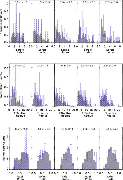
The single Sérsic model fit parameter distributions for the control sample in grey, overplotted by those for the AGN hosts in blue. The top row shows the Sérsic index distributions, the middle row shows the effective radii distributions in units of kpc and the bottom row shows the axial ratio distributions. These distributions have been normalized so that the area under each histogram is equal to one in order to facilitate comparison between the AGN host sample and the much larger control sample. They reveal trends for the AGN hosts to have higher Sérsic indices at z > 1.5. We do not find any significant evidence that the effective radii of the AGN hosts and control samples differ. However, we do report that the axial ratio distributions of the two populations are inconsistent in the 1.5 < z < 2 bin, with the AGN hosts displaying a distribution with rounder systems than the control sample.
In agreement with Rosario et al. (2015) for the same CANDELS GOODS-S data set, we observe that at the highest redshifts probed here the AGN hosts display a statistically distinguishable Sérsic index distribution, where the AGN host distribution is centred on higher index values, meaning that the hosts have morphologies with larger bulge contributions than the non-active control sample.
For the purposes of this analysis, we consider only the Sérsic index fits in the range 0.2 ≤ n ≤ 8, which is commonly adopted as a meaningful range of parameter values in the literature. For completeness, we have conducted our K–S tests using the 0 < n < 20, n ≥ 0.2 and n ≤ 8 parameter ranges and find that they are all formally significant in the z > 1.5 bins, but in order to be conservative, here we report only the results for the 0.2 ≤ n ≤ 8 fits. The K–S p values for AGN host and non-active control sample Sérsic index distributions in each redshift bin are listed in Table 1, where it can be seen that, above z ∼ 1.5, the AGN hosts and the non-active control sample are distinguishable at the 95 per cent confidence level.
The one-dimensional K–S test p values for the distributions of the: 0.2 ≤ n ≤ 8 Sérsic indices, effective radii and axial ratios of the AGN hosts and the mass-matched control galaxies from the single Sérsic model fitting. The sample size of the X-ray-selected AGN sample is included in the bottom row.
| Parameter | 0.5 < z < 1 | 1 < z < 1.5 | 1.5 < z < 2 | 2 < z < 2.5 | 2.5 < z < 3 |
|---|---|---|---|---|---|
| n | 0.248 | 0.511 | 0.002 | 0.018 | 0.004 |
| re | 0.151 | 0.851 | 0.851 | 0.781 | 0.126 |
| Axial ratio | 0.106 | 0.461 | 0.004 | 0.09 | 0.175 |
| X-ray sample | 20 | 17 | 44 | 25 | 35 |
| Parameter | 0.5 < z < 1 | 1 < z < 1.5 | 1.5 < z < 2 | 2 < z < 2.5 | 2.5 < z < 3 |
|---|---|---|---|---|---|
| n | 0.248 | 0.511 | 0.002 | 0.018 | 0.004 |
| re | 0.151 | 0.851 | 0.851 | 0.781 | 0.126 |
| Axial ratio | 0.106 | 0.461 | 0.004 | 0.09 | 0.175 |
| X-ray sample | 20 | 17 | 44 | 25 | 35 |
Within these panels the well-known evolution of massive galaxies within this redshift regime from disc to bulge-dominated (Buitrago et al. 2008; Bruce et al. 2012) systems can also clearly be seen which, coupled with the comparison of the Sérsic index distributions of the AGN and control sample suggests that the AGN hosts may have an accelerated evolution, building up a significant bulge at earlier epochs compared to their mass-matched non-active analogues. However, overall it appears to suggest that the physical processes driving the evolution of these active and non-active systems are similar. Given the current evidence, from studies into the connection between galaxy star formation rates and morphologies (e.g. Bruce et al. 2012; McLure et al. 2013; Mancini et al. 2015) in favour of a scenario where discs evolve through violent disc instabilities to gradually build up massive bulges rather than exclusively through gas-poor major mergers, this further suggests that major mergers may not play the dominant role in triggering AGN, as also commented on by Rosario et al. (2015).
A comparison of the effective radii and axial ratio distributions for the fits reveals no evidence for any offset in the effective radii distributions for the AGN host and non-active control samples. For the axial ratio distributions, the K–S test for the non-active control sample and AGN host galaxies returns a low p value in the 1.5 < z < 2 redshift bin. However, we do not find evidence for a consistent difference in the distributions of these two samples in other redshift bins so do not ascribe any importance to this result.
4.3 The addition of point-source models
We next explore how the addition of a point-source component in our model affects the fitted morphologies of the AGN and the control sample. For this analysis, we adopt the procedure implemented in Bruce et al. (2012), where we only adopt a more complex model if it contains ≥10 per cent of the overall flux of the object and if the addition of the component reduces the χ2 value of the fit by more than expected given the increased degrees of freedom. Therefore, the results that we present in this section are updated only with the objects that require a point-source component in order to be better modelled. They do not illustrate the effect of imposing a point source in the models of all objects. In this way, we allow the data to drive the level of morphological decomposition and do not make any a priori assumptions about certain samples, for example assuming that all AGN hosts should be fit with point-source components.
From the best-fitting models with the inclusion of a point-source component, we still see the same trend for AGN hosts to have higher bulge fractions than the control sample, where again from the adoption of our test, we conclude that the AGN host and control sample Sérsic index distributions become distinguishable at the 95 per cent confidence level above z = 1.5. The tabulated K–S p values for the AGN host and control sample Sérsic index, effective radii and axial ratio distributions, now for the best-fitting single Sérsic + point-source fits, are given in Table 2, and the full distributions are plotted in Fig. 3.
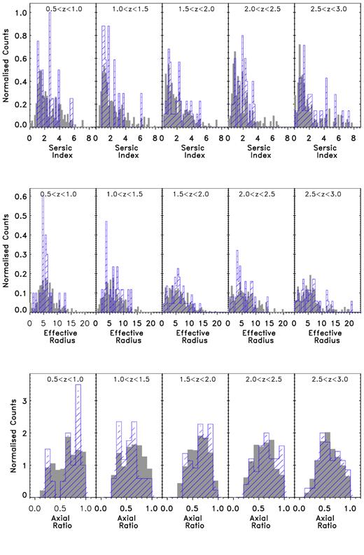
In comparison to Fig. 2, these plots show the single Sérsic + point-source model fit parameter distributions. Again, the control sample results are plotted in grey and are overplotted by those for the AGN hosts in blue. The top row shows the Sérsic index distributions, the middle row shows the effective radii distributions and the bottom row shows the axial ratio distributions. As with Fig. 2, these distributions have been normalized so that the area under each histogram is equal to one. The same trends witnessed in Fig. 2 exist in the highest redshift bin here with the single Sérsic + point-source model fits and are still formally significant.
The one-dimensional K–S test p values for the distributions of the: 0.2 ≤ n ≤ 8 Sérsic indices, effective radii and axial ratios of the AGN hosts and the mass-matched control galaxies, now from the single Sérsic + point-source model fitting. The probability of three contiguous redshift bins displaying p < 0.05, for any parameter, is ≤0.000 01, indicating that the trend for the AGN hosts to be more bulge dominated than the general galaxy population at high redshift is highly significant (see text for details).
| Parameter | 0.5 < z < 1 | 1 < z < 1.5 | 1.5 < z < 2 | 2 < z < 2.5 | 2.5 < z < 3 |
|---|---|---|---|---|---|
| n | 0.342 | 0.225 | 0.015 | 0.038 | 0.002 |
| re | 0.341 | 0.901 | 0.197 | 0.836 | 0.085 |
| Axial ratio | 0.07 | 0.461 | 0.004 | 0.141 | 0.301 |
| Parameter | 0.5 < z < 1 | 1 < z < 1.5 | 1.5 < z < 2 | 2 < z < 2.5 | 2.5 < z < 3 |
|---|---|---|---|---|---|
| n | 0.342 | 0.225 | 0.015 | 0.038 | 0.002 |
| re | 0.341 | 0.901 | 0.197 | 0.836 | 0.085 |
| Axial ratio | 0.07 | 0.461 | 0.004 | 0.141 | 0.301 |
This can be seen in more detail when we look at the cumulative distributions of the two samples, as displayed in Fig. 4. From these plots, it is clear that the differences between the Sérsic index distributions of the two samples occur due to the AGN hosts (in red) having relatively fewer low Sérsic index fits and more high Sérsic index fits compared to the non-active control sample.
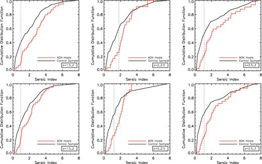
The cumulative distribution functions for the Sérsic indices for the single Sérsic best-fitting models on the top row and for the best-fitting single Sérsic + point-source models in the bottom row. The AGN hosts are plotted in red and the control sample is overplotted in black. The indices at which the largest deviation between the distributions occurs are marked by the vertical dashed, grey line. We note that, to be consistent with Tables 1 and 2, we plot only the 0.2 ≤ n ≤ 8 Sérsic index range. These plots highlight that the largest differences in the distributions between the active and non-active samples occur at low Sérsic indices, where the AGN hosts display a lower overall contribution from low index (i.e. more disc-dominated) fits, indicating that the AGN host structures have a larger contribution from a bulge component.
As discussed above, by constructing a maximally mass-matched control sample and comparing the AGN host galaxy structural parameters to those of the medians of the 1000 times bootstrapped control samples, the statistical significance of these trends is measured with the relatively small number of AGN host galaxies within each redshift bin.
As a result, we have tested the statistical significance of the trend for AGN hosts to have more bulge-dominated Sérsic indices than the mass-matched control sample, by rejecting our null hypothesis that these two distributions are drawn from the same parent distribution for p values more extreme than the critical value of 0.05 from the K–S test, corresponding to the 95 per cent confidence level. However, we do note that this trend is witnessed in three consecutive redshift bins at z ≥ 1.5.
To quantify the significance of this coherent trend we utilize the Monte Carlo calculations outlined at the beginning of this section, where we calculated the probability of any occurrence of p < 0.05 in any three consecutive redshift bins for any morphological parameter. The result of this calculation is the probability ∼0.000 01 that this type of redshift coherent pattern could emerge by chance.
This confirms that the morphologies of the AGN hosts do indeed intrinsically have higher contributions from a bulge component than the control sample of non-active galaxies and this trend is not a result of any bias from overlooked centrally concentrated contributions from the AGN itself.
4.4 Multiple Sérsic models
Given the differences in the morphologies of the AGN hosts and the control sample indicated from a single Sérsic fit to the data, we now explore these trends in more detail with a full bulge-disc decomposition of both samples. The methodology for choosing best-fitting models from our decompositions was previously developed for a high-mass (M > 1011 M⊙) sample with higher S/N than the M > 1010 M⊙ sample selected for this work. As a result, when applied to this sample, we found that the |$\chi ^{2}_{{\rm complex}} <\chi ^{2}_{{\rm simple}}-\Delta \chi ^{2}(\nu _{{\rm complex}}-\nu _{{\rm simple}})$| criteria imposed to adopt more complex models was too stringent and returned best fits which were limited to single components. While these fits may be the most statistically validated fits on an object-by-object basis, it is clear they do not best represent the morphologies of the overall population. For this reason, for the multiple component fits for this lower mass sample of both AGN hosts and the non-active control sample we relax the χ2 criteria and simply adopt as best-fit the model with the lowest χ2 value, but still ensure that any component is ≥10 per cent of the overall flux of the object. Having tested this approach on the high-mass end of this sample, we have ensured that the relaxation of the χ2 criteria does not bias the fits towards any non-physical model set-up, for example, disc-dominated bulge+disc objects are best fit with pure discs when the criteria are strengthened and vice versa.
The bulge and disc light fraction distributions obtained from this approach are shown in Fig. 5. Again, here the results presented depict the best-fitting morphologies which have the option to adopt a point-source component where motivated by the data.
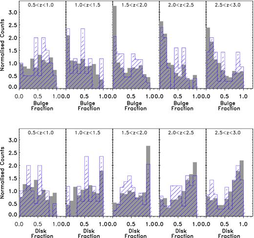
The light fraction distributions from our full morphological decomposition for the control sample in grey, with the distributions for the AGN hosts overplotted in blue. The bulge component light fractions are given in the upper row and the disc component in the lower row. The histograms have been normalized to be consistent with those in Figs 2 and 3. Above z = 2.5, these distributions reveal that the AGN hosts have fewer low-bulge components and more lower disc components than the control sample. However, these trends are more easily seen in the cumulative distribution functions shown in Figs 6 and 7.
From a one-dimensional K–S test of the AGN hosts and the median of the 1000 bootstrapped mass-matched control samples, we can again reject our null hypothesis for the bulge light fractions at the 95 per cent confidence level above z = 2.5. From the cumulative distribution functions, Fig. 6 for the bulge light fractions and Fig. 7 for the disc light fractions, we can see that the AGN host sample displays fewer low-bulge fraction components and more low disc fraction components, in additional to more pure bulges systems. Therefore, this further corroborates our findings that, even when fully decomposed, the AGN hosts have higher bulge fractions than a mass-matched non-active control sample.
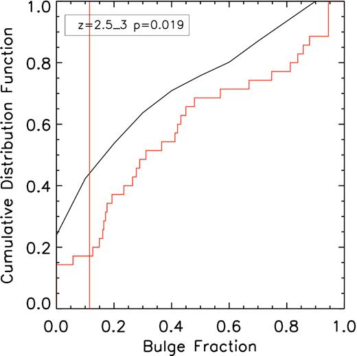
The cumulative distribution function for the bulge component light fractions. The AGN hosts are given in red, and the control sample light fractions are shown in black. The red vertical line represents the bulge fraction at which the biggest difference between the cumulative distribution functions occurs. From these plots, it is clear that the differences in these distributions arises due to the AGN hosts having fewer low-bulge fraction components, and also more high-bulge fraction components.
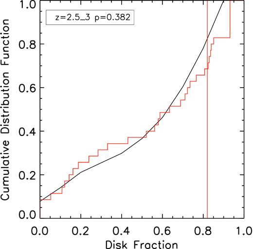
Following on from Fig. 6, this plot shows the cumulative distribution function of the disc component light fractions. Again the distribution function of the AGN hosts is plotted in red and that of the control is in black. The red vertical line represents the disc fraction at which the biggest difference between the cumulative distribution functions occurs. Comparison of these distributions reveals that in addition to the AGN hosts having more low disc fraction components, they also have fewer high disc fraction components, consistent with the claim that the AGN hosts have higher bulge fractions than the non-active control sample.
Finally, we address the issue of morphological K-corrections within our 0.5 < z < 3 range. It is clear that the adoption of our H160-band morphological classifications probes increasingly bluer rest-frame light at higher redshifts. It is possible that this may contribute to the higher bulge fractions observed in the AGN host sample compared to the control sample if the contribution to nuclear light from the AGN itself becomes more dominant at the bluer wavelengths probed by our fixed-band morphological decomposition at higher redshifts. However, from our detailed multi-wavelength decompositions, we do not find any such differences in the broad-band SEDs of the control sample galaxies compared to the X-ray identified AGN hosts for the majority of objects. Thus, we conclude that there is no evidence to suggest that the H160-band morphologies of the AGN hosts are more biased by contributions from the AGN itself at higher redshifts, and so we do not consider this as a major concern. Moreover, we find no trend for the point-source fits to be adopted with higher frequency, or to have higher point-source fractions, at high redshifts compared to lower redshifts.
4.5 The role of the galaxy bulge in determining AGN activity
Given that we have determined robust H160-band light fraction decomposed stellar masses for our AGN sample, we are also able to address the issue of whether the BH mass shows a stronger trend with the bulge as opposed to the total stellar mass of the host. Determining BH mass estimates from dynamical measurements is beyond the scope of this work. However, we can further exploit our comparison between the total masses and decomposed bulge masses of our AGN hosts and of our full M* > 1010 M⊙ sample in order to shed some light on this issue.
In Fig. 8, we present the binned bulge fractions of the AGN hosts (in blue) and the full sample (in black) as a function of the total stellar masses of the systems. Both the mean (large circles), median (small squares) and interquartile ranges have been displayed in the figure to allow a full comparison of the distribution of bulge fractions for the two populations. As a reminder, we have selected this sample via a mass and photo-z selection cut at M* > 1 × 10¹⁰ M⊙ with 0.5 < z < 3, and have cross-matched these objects with the full Hsu et al. (2014) 4Ms Chandra X-ray-selected counterpart catalogue. Thus, the higher bulge fractions displayed in the lower mass AGN hosts compared to the non-active galaxies suggest that in order to have been included in an X-ray flux limited catalogue, the lower mass AGN hosts had to have a larger contribution from a bulge component. When viewed in light of the strong trend between bulge mass and total stellar mass, this shallower evolution in bulge mass with total stellar mass for the low-mass AGN hosts compared to the non-active sample indicates that the X-ray luminosity, and therefore BH mass, is more correlated with the bulge stellar mass of the hosts than the total mass.
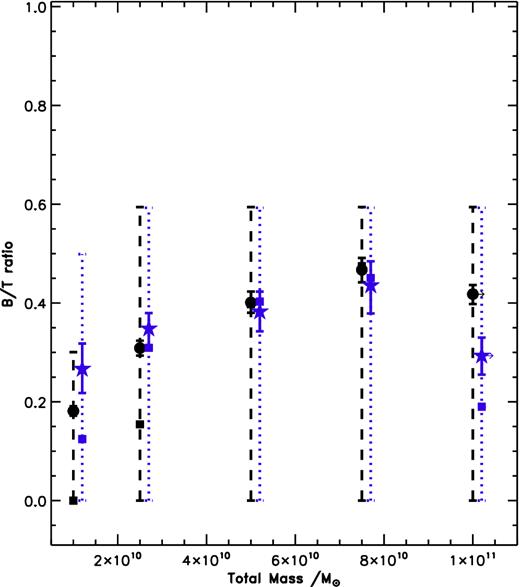
The binned bulge fractions of the AGN and the full CANDELS GOODS-S, 0.5 < z < 3, M* ≥ 1 × 10¹⁰ M⊙ non-active galaxies as a function of the total stellar mass in the systems. Here the mass bins are ΔM* = 2.5 × 10¹⁰ M⊙ in size and extend to M* = 1 × 10¹¹ M⊙ at which point all higher mass systems are included in the M* ≥ 1 × 10¹¹ M⊙ bin in order to maintain a reasonable number of objects in each bin. The AGN hosts are displayed in blue and the full non-active, M* > 1010 M⊙, sample is shown in black. The large circles represent the mean bulge fractions in the bin, whereas the small squares are the median values. The interquartile ranges are also given by the dotted and dashed lines for the AGN and non-active galaxies, respectively, and have been offset to allow for clearer viewing. From this comparison, we can see that the lower mass AGN hosts have a higher mean and median bulge fraction than the non-active control sample.
This exploration of the bulge and total stellar mass distributions for the AGN hosts and control sample also provides clarity on the effectiveness of our M* > 1 × 10¹⁰ M⊙ galaxy cut at encompassing the majority of the X-ray-identified AGN from the counterpart catalogue of Hsu et al. (2014). As we can see from Fig. 9, within the scatter, the bulge stellar mass distribution of the AGN host population truncates at higher bulge mass than the overall galaxy population. In addition to this, looking at the overall distributions, the AGN hosts have higher median bulge stellar masses (log 10(M*/M⊙) = 10.51 in both redshift bins) compared to the control samples (log 10(M*/M⊙) = 10.33 and log 10(M*/M⊙) = 10.32 for the low- and high-redshift bins, respectively). Thus, it is clear that systems with bulge masses >1 × 10¹⁰ M⊙ are needed in order to fully represent the AGN host population within a mass-matched sample and in fact this correlation with higher bulge masses may be the reason for the well-known trend for AGN hosts to be biased towards higher total stellar masses than the underlying galaxy population within a given mass-cut sample.
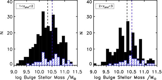
The bulge stellar mass distributions for the full CANDELS-GOODSS, 0.5 < z < 3, M* ≥ 1 × 10¹⁰ M⊙ galaxy population in black, overplotted with the AGN host sample in blue, at two different redshift intervals. The medians of the two distributions have been overplotted in the blue and black dashed lines for the AGN hosts and control sample, respectively. These distributions indicate that the AGN hosts have fewer low-bulge stellar mass systems, thus suggesting that the M* = 1 × 10¹⁰ M⊙ mass-cut maximizes the overlap with the X-ray-selected AGN host sample of Hsu et al. (2014) due to the fact that the inclusion of M* > 1 × 10¹⁰ M⊙ bulge stellar masses systems is needed to properly sample the AGN host galaxy population. Furthermore, this trend in bulge stellar masses may also play an important role in the observation that generally AGN hosts are biased towards higher total stellar masses within a more general mass-cut galaxy sample.
5 NATURE OF THE POINT-SOURCE COMPONENT
Having determined that the trend for X-ray-selected AGN host galaxy morphologies to be more bulge dominated at high redshifts is not an artefact of the poor fitting of any contribution from the AGN itself to the near-IR photometry of these objects, we now turn our attention to the physical nature of the point-source component adopted in some of the fits, and ask how well this correlates with the presence of an AGN.
5.1 Point-source fraction differences
It is clear from this, and our previous (Bruce et al. 2012, 2014) studies, that a significant fraction of massive galaxies require a point-source component in order to best fit their light profiles. So how does the fraction of point-source fits in the mass-matched control sample compare to that in the X-ray-selected AGN hosts? In Fig. 10, we show the cumulative distribution functions of the point-source light fractions in each redshift bin for the AGN hosts in red and the mass-matched control sample in black, and overplot in each panel the one-dimensional K–S test p values for the distributions. This demonstrates that, overall, we fail to reject the null hypothesis that the distributions of the point-source fractions are drawn from the same distribution at the 95 per cent confidence level, thus revealing that there is no evidence for the AGN hosts to be more point-source dominated than the non-active control sample.
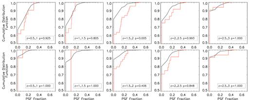
This figure demonstrates the similarity in the point-source light fractions between the AGN hosts and the control sample for both the single Sérsic + point-source fits and the fully decomposed bulge+disc+point-source fits. As with the previous plots, the cumulative distribution functions for the AGN are shown in red and those for the control sample are plotted in black. The point-source light fractions from the single Sérsic + point-source fits are plotted in the top row, and the fits from the full morphological decomposition are given in the bottom row. These plots serve to illustrate that there is no significant difference in the point-source light fractions between the active and non-active samples, thus suggesting that there is no strong correlation between the presence of a point-source fit in the data with X-ray-selected AGN activity.
We explore this result further by splitting our X-ray-selected AGN hosts into obscured and unobscured sub-sets using both the X-ray spectra, implementing hardness ratio cuts and the effective photon index cuts from Xue et al. (2011), and alternatively via optical spectra classifications from Szokoly et al. (2004). In doing so, we do not find a formally significant difference (p = 0.07) in the point-source fractions for the X-ray-defined obscured and unobscured sub-sets. Splitting by optical classifications does not reveal any difference between the point-source fractions of the obscured and unobscured subsets (p = 0.96). Looking further into the trends between the optical classifications of the X-ray-selected AGN and the prevalence of a point-source fit in their morphologies, we also observe no clear trend between the brightest Quasi-Stellar objects and point-source fractions. However, (as can be seen in Fig. 11) by splitting the AGN sample at LX = 1 × 1043.5 erg s−1, the limit above which traditionally AGN contamination is thought to become a concern at X-ray luminosities, we do find some evidence that the most luminous AGN have higher point-source light fractions, by once more adopting our test and rejecting the null hypothesis from a K–S test at the 95 per cent confidence level.
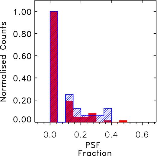
The point-source light fractions of the X-ray-selected AGN sample split into low X-ray luminosity, LX < 1 × 1043.5 erg s−1 (red) and high-luminosity LX > 1 × 1043.5 erg s−1 (blue) using samples. These distributions have been normalized such that the maximum bin value is set equal to one. This plot reveals that the higher X-ray luminosity AGN have higher point-source light fractions compared to the lower luminosity sample.
As an aside, on an object-by-object basis, 9.7 ± 0.8 per cent of all galaxies are best fit with a point-source component compared to 13.4 ± 2.4 per cent of all X-ray-selected AGN hosts. This suggests a marginal preference for AGN hosts to be more point-source dominated, but as mentioned previously, there are mass biases implicit in this comparison which make it less than ideal.
From these comparisons, we see no definitive confirmation that the point-source fits correlate with either the presence of an X-ray-selected AGN, or within the AGN sample with the AGN obscuration, as might be expected.
5.2 Stacking of X-ray images
In order to ensure this result is not biased by point-source fits which are AGN with faint X-ray signatures below the detection limit of the Xue et al. (2011) catalogues, we have constructed stacks of the X-ray image at the CANDELS positions of the sources with: the 10 brightest point-source components; and with the 10 largest point-source fractions. For direct comparison, we also stack 10 non-point source fits with no X-ray detections in the catalogue with similar redshifts, masses, magnitudes and sizes as the point-source sample in order to construct a control set. The stacks have been created from a mean combination.
The stacks are displayed in Fig. 12 with the top row for the brightest point-source fits and the bottom row for the point-source fits with the highest light fractions. The stamps on the left are the mean stacks of the point-source fits with no X-ray detections and the stamps on the left illustrate the control samples for both cases. Aperture photometry on these stacks reveals no significant evidence for more flux in the stacks of the highest point-source light fractions sample than in the stacks of the control sample.

The ∼2 arcsec × 2 arcsec X-ray-stacked images of the various sub-samples probed in order to explore the possibility of point-source model fits picking up faint AGN below the detection limits of the (Xue et al. 2011) X-ray-selected catalogue. From left to right are: the mean combined stacks of the 10 brightest PSF fits without X-ray counterparts and the associated non-point-source control sample, then the stacks of the 10 highest fraction point-source fits without X-ray detections and the control sample. Here we can see no evidence for excess flux in the stacks of either of the point-source model samples and as a result conclude that the point-source fits are not indicative of AGN activity in the X-ray below the limit of current surveys.
5.3 Further connections between point source and X-ray properties
In the previous section, we have concluded that, by comparing the point-source fractions between AGN hosts and a mass-matched control sample there is no evidence for a correlation between the prevalence of a point-source fit and an AGN detection, even when stacking the X-ray to search for low luminosity sources. However, another correlation to test for is the link between the point-source luminosity and the luminosity of the AGN detected in the X-ray, which should shed light on whether the point-source fit is related to AGN activity (in which case, one would expect a scaling between point-source luminosity and AGN X-ray luminosity) or whether it is a signature of a nuclear starburst in the system.
This comparison is given in Fig. 13, now on an object-by-object basis. Here we plot the objects with X-ray detections and point-source component fits, as well as point-source fits with no X-ray counterparts in colour, where red represents bulge+PSF fits, blue represents disc+PSF fits and bulge+disc+PSF fits are plotted in green. Objects with an X-ray detection and no point-source fits are plotted in grey. There is significant scatter in this plot but there is a positive correlation between the point-source luminosity and the AGN X-ray luminosity, which can be fitted with a Spearman Rank correlation coefficient ρ = 0.31 with p < 0.005. When binned, as shown in purple, we find that the correlation between the mean values in each bin is weaker and no longer statistically significant: ρ = 0.143 with p > 0.25.
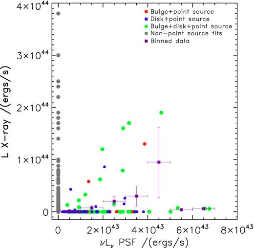
This figure explores the potential correlation between the AGN X-ray luminosity and the point-source luminosity in the H160 band. Objects which have a point-source fit with or without an X-ray counterpart are colour coded: red for bulge+point-source fits, blue for disc+point-source fits and green for bulge+disc+point-source fits. Objects which have an X-ray counterpart with no point-source fit are coloured grey. We also overplot in purple the binned mean of the X-ray luminosity in each point-source luminosity bin with error bars representing the standard error on the mean.
To explore this potential connection further we have also looked at the fractions of point-source components which have X-ray counterparts (Fig. 14). Whilst there is tentative evidence here that the fraction of point-source components with X-ray counterparts increases with the luminosity of the point source, the errors on these fractions are large as they are driven by the scatter within the sample.
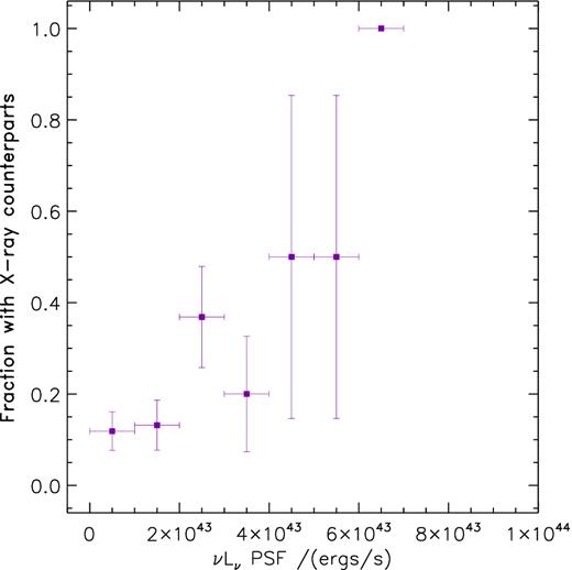
Plot demonstrating the fraction of point-source fits with an X-ray counterpart as a function of the point-source component luminosity. These results suggest that the most luminous point-source fits are the most likely to host AGN.
Conversely, it would seem that the fraction of X-ray sources with a point-source component fit (Fig. 15) correlates with the moderate luminosity AGN but then falls off at higher AGN X-ray luminosities. Moreover, this trend is unaffected if the AGN sample is split according to effective photon index into obscured and unobscured sub-samples.
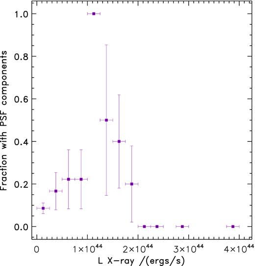
In contrast to Fig. 14, here we present the fraction of X-ray counterparts with point-source fits as a function of the X-ray luminosity. Now we see a turnover at moderate luminosity: below which there appears to be a general trend towards more luminous AGN having an increased likelihood of point-source component fits; and above which the opposite is the case.
In conclusion, there does not appear to be a strong correlation between the adoption of a point-source component in the morphological fitting and the presence of an AGN. However, there is some indication that by selecting the brightest point-source component fits, one is more likely to be preferentially selecting AGN hosts, but this bright point-source fit sub-set may also contain non-active galaxies.
6 CONCLUSIONS
We have presented an analysis of the rest-frame optical morphologies of AGN hosts in the CANDELS GOODS-S field in the redshift range 0.5 < z < 3 with masses M* > 1010 M⊙ and compared them to a carefully mass-matched control sample of non-active galaxies. Having explored the effects of fitting either single Sérsic, multiple Sérsic and models with point-source components, we confirm that the AGN hosts are indeed more bulge dominated in the highest redshift bins (z ≥ 2) than the non-active control sample, as has been reported from previous studies. We conclude that morphological fits of AGN without the addition of point-source components to model any nuclear light from the AGN do not bias this overall trend towards AGN hosts being more bulge dominated. Furthermore, when fully decomposed into their separate components, it is clear that the AGN hosts have significant bulge and disc components.
This is suggestive of the fact that both of these stellar populations play an important role in the triggering of AGN, with not only the bulge component being crucial to feed the central BH, but a massive disc being necessary to support the growth of the bulge.
By demonstrating that the AGN hosts display massive disc components and that the overall evolution of the AGN hosts across the 0.5 < z < 3 range is comparable with that, although may be accelerated in comparison to, the non-active control galaxies, our findings are consistent with a scenario in which secular processes are responsible for the triggering of moderate luminosity AGN at z ≥ 1.
From a full exploration of the correlation between point-source fits in a purely mass-selected sample of galaxies and the prevalence of AGN activity within these sources, we do not find strong evidence in favour of the point sources being AGN in nature. In fact, there is considerable evidence from the colours of the point-source fits, as will be shown in a companion paper (Bruce et al., in preparation) with a full exploration of the trends between the fitted ages, dust obscuration values and morphologies, that they are in fact nuclear starbursts. Consequently, the adoption of the point-source fits in both the active and non-active control samples should be used to best describe the full stellar structure of these systems.
Finally, from a comparison of the total stellar mass and bulge stellar mass trends within our full mass-selected and AGN host samples, we find evidence in this redshift regime that the BH mass may be better correlated with the bulge mass than the total stellar mass of these systems. Furthermore, we also find evidence that the trend for AGN hosts to have a higher low-end cut-off in bulge stellar mass than the underlying galaxy population may play a role in the more general observation that AGN hosts are biased towards higher total stellar masses compared to the underlying galaxy population within a mass-cut sample.
We thank the referee for a careful, critical, but ultimately constructive review of this work which helped to clarify the statistical significance of our results. VAB and JSD acknowledge the support of the EC FP7 Space project ASTRODEEP (Ref. No: 312725). JSD acknowledges the support of the European Research Council via the award of an Advanced Grant. AM acknowledges funding from the STFC and a European Research Council Consolidator Grant (P.I. R. McLure).
This work is based in part on observations made with the NASA/ESA HST, which is operated by the Association of Universities for Research in Astronomy, Inc, under NASA contract NAS5-26555. This work is based in part on observations made with the Spitzer Space Telescope, which is operated by the Jet Propulsion Laboratory, California Institute of Technology under NASA contract 1407.
REFERENCES
