


Abstract
We present a spectroscopic survey of known and candidate γ Doradus stars. The high-resolution, high signal-to-noise spectra of 52 objects were collected by five different spectrographs. The spectral classification, atmospheric parameters (Teff, log g, ξ), vsin i and chemical composition of the stars were derived. The stellar spectral and luminosity classes were found between G0–A7 and IV–V, respectively. The initial values for Teff and log g were determined from the photometric indices and spectral energy distribution. Those parameters were improved by the analysis of hydrogen lines. The final values of Teff, log g and ξ were derived from the iron lines analysis. The Teff values were found between 6000 K and 7900 K, while log g values range from 3.8 to 4.5 dex. Chemical abundances and vsin i values were derived by the spectrum synthesis method. The vsin i values were found between 5 and 240 km s−1. The chemical abundance pattern of γ Doradus stars were compared with the pattern of non-pulsating stars. It turned out that there is no significant difference in abundance patterns between these two groups. Additionally, the relations between the atmospheric parameters and the pulsation quantities were checked. A strong correlation between the vsin i and the pulsation periods of γ Doradus variables was obtained. The accurate positions of the analysed stars in the Hertzsprung–Russell diagram have been shown. Most of our objects are located inside or close to the blue edge of the theoretical instability strip of γ Doradus.
1 INTRODUCTION
The class of γ Doradus (γ Dor) variables was defined by Balona, Krisciunas & Cousins (1994) after discovery of the variability of the prototype of these pulsators (Cousins 1992; Krisciunas et al. 1993). The γ Dor variables exhibit pulsations in the non-radial, high-order (n), low-degree (l) gravity modes with amplitudes at the level of 0.1 mag (V) and pulsation periods between 0.3 and 3 d (Kaye et al. 1999). The pulsations of γ Dor stars are driven by the mechanism of convective flux blocking (Guzik et al. 2000; Dupret et al. 2005). In the Hertzsprung–Russell (H-R) diagram, the theoretical instability strip of γ Dor variables is located partially inside the instability strip of δ Scuti (δ Sct) stars. In this small overlapping part, the existence of stars pulsating simultaneously in both δ Sct and γ Dor modes was predicted (Dupret et al. 2004). These stars are called γ Dor/δ Sct or A-F type hybrids. The γ Dor variables are A7-F5 dwarfs and/or subdwarfs (Kaye et al. 1999). This means that in the H-R diagram they are situated inside the region of the transition from a convective envelope to a convective core. In order to reveal properties of the pulsation mechanism in F type stars and to decide on the correct location of the theoretical instability strip of γ Dor stars in the H-R diagram, the interaction between convection and pulsation has to be taken into account (Saio et al. 2015). Moreover, the investigation of γ Dor variables allows us to examine important subjects of the internal structure and evolution of intermediate mass stars (Miglio et al. 2008). In particular, the frequency spacing detected in the photometric time series has allowed the study of the internal structure and surface-to-core rotation (e.g. Kurtz et al. 2014; Van Reeth et al. 2015).
In-depth studies of the pulsating A-F type stars have now become possible due to the space observations. In particular, the high-precision light curves of the Kepler mission enabled investigation of many new A-F type variables (Borucki et al. 2010). Before the space observations, approximately 100 γ Dor stars were known (Henry, Fekel & Henry 2011). The analysis of the Kepler data revealed many new candidate γ Dor, δ Sct and A-F type hybrid stars (Grigahcène et al. 2010; Uytterhoeven et al. 2011a). The investigation of Kepler observations and ground-based photometric data allow us to determine pulsation characteristics, ranges of fundamental parameters, and position of these variables in the H-R diagram.
However, many new questions about the properties of the γ Dor stars, δ Sct stars and their hybrids arose. The first question concerns the exact location of the instability domains of these variables in the H-R diagram. According to the existing studies, there seems to be no clear distinction in the edges of the observational instability strip of γ Dor and δ Sct stars. Moreover, it was shown that candidate hybrids of γ Dor and δ Sct stars were detected everywhere inside the theoretical instability strips of both types of pulsating stars (e.g. Kurtz et al. 2014; Niemczura et al. 2015). Another question relates to the chemical structure of the hybrid stars. Some Am hybrid stars were discovered, and these results showed that a relation between the Am phenomenon and hybridity could exist (Hareter et al. 2011). Solving these problems requires investigation of whether chemical and physical differences between hybrids, γ Dor, and δ Sct variables exist. Therefore, it is necessary to obtain the accurate physical and chemical characteristics of all classes of A-F type variables. Hence, reliable spectroscopic and multicolour photometric studies are essential.
So far, several photometric and spectroscopic studies of γ Dor stars have been carried out (e.g. Mathias et al. 2004; Henry, Fekel & Henry 2007). One of the most detailed spectroscopic investigations of γ Dor stars was presented by Bruntt, De Cat & Aerts (2008). They derived fundamental atmospheric parameters and chemical composition of bona-fide and candidate γ Dor stars to search for links between γ Dor, Am and λ Boötis stars, but no relations were found. Additionally, detailed spectroscopic analyses of γ Dor stars detected in satellite fields have been carried out (e.g. Tkachenko et al. 2012, 2013a; Niemczura et al. 2015; Van Reeth et al. 2015). In these studies, the fundamental atmospheric parameters and chemical abundances of these variables were derived.
The aim of this study is to obtain the atmospheric parameters and chemical abundances of some bona-fide and candidate γ Dor stars detected from the ground-based observations. Therefore, we gathered high-resolution and high signal-to-noise (S/N) spectra for 69 γ Dor stars using five different spectrographs from around the world. This sample contains a mixture of single stars, single-lined binaries (SB1) and double-lined spectroscopic binaries (SB2). The analysis of SB2 γ Dor stars will be presented in a separate paper (Kahraman Aliçavuş et al., in preparation). In this study, a detailed spectroscopic analysis of 52 single and SB1 γ Dor stars is performed. The high-resolution observation, data reduction and calibration details are given in Section 2. Spectral classification process is described in Section 3. Determination of the atmospheric parameters from photometric systems and spectral energy distribution (SED) are presented in Section 4. In Section 5, we introduce the atmospheric parameters determination from the analysis of hydrogen and iron lines, the detailed chemical abundance analysis, and discussion of the obtained parameters. The summary of the results and an outlook for future studies are given in Section 6.
2 OBSERVATIONS
The observations of our targets were carried out with five high-resolution spectrographs. Numbers of the observed single & SB1 and SB2 stars, observation years, spectral resolutions of instruments, wavelength range and S/N ranges are given in Table 1. For each spectrograph, the listed S/N range gives the maximum and minimum value of S/N at 5500 Å. The following instruments were used in the survey:
(i) FEROS (Fibre-fed Extended Range Optical Spectrograph), an échelle spectrograph attached to the 2.2-m telescope of the European Southern Observatory (ESO, La Silla, Chile; Elkin, Kurtz & Nitschelm 2012);
(ii) FIES (Fibre-fed Échelle Spectrograph), a cross-dispersed high-resolution échelle spectrograph attached to the 2.56-m Nordic Optical Telescope of the Roque de los Muchachos Observatory (ORM, La Palma, Spain; Telting et al. 2014);
(iii) HARPS (High Accuracy Radial Velocity Planet Searcher), an échelle spectrograph attached to the 3.6-m telescope of the ESO (La Silla, Chile; Mayor et al. 2003);
(iv) HERCULES (High Efficiency and Resolution Canterbury University Large Échelle Spectrograph), a fibre-fed échelle spectrograph attached to the 1-m McLellan telescope of the Mt. John University Observatory (MJUO, Mount John, New Zealand; Hearnshaw et al. 2003);
(v) HERMES (High Efficiency and Resolution Mercator Échelle Spectrograph), a high-resolution fibre-fed échelle spectrograph attached to the 1.2-m Mercator telescope at the Roque de los Muchachos Observatory (ORM, La Palma, Spain; Raskin et al. 2011).
Information about the spectroscopic observations.
| Instrument | Number of | Years of | Resolving | Spectral | S/N |
|---|---|---|---|---|---|
| single & SB1/SB2 stars | observations | power | range [Å] | range | |
| FEROS | 0 / 8 | 2008 | 48 000 | 3500–9200 | 170–340 |
| FIES | 29 / 2 | 2007–2010 | 67 000 | 3700–7300 | 100–330 |
| HARPS | 11 / 4 | 2009–2011 | 80 000 | 3780–6910 | 130–360 |
| HERCULES | 11 / 3 | 2007–2010 | 70 000 | 4000–8800 | 110–300 |
| HERMES | 1 / 0 | 2010 | 85 000 | 3770–9000 | 150 |
The collected spectra have been reduced and calibrated using the dedicated reduction pipelines of the instruments. The usual reduction steps for échelle spectra were applied, i.e. bias subtraction, flat-field correction, removal of scattered light, order extraction, wavelength calibration, and merging of the orders. For the HERCULES data, an additional procedure had to be used to merge the échelle orders. In this procedure, the overlapping parts of the orders were averaged using the S/N of the given order as the weight. The normalization of all spectra was performed manually by using the continuum task of the NOAO/iraf package.1
Some of the studied stars were observed by more than one instrument. In this case, only the spectra of the instrument with the highest resolution were analysed. For some of the stars, we collected more than one spectrum from the same instrument. For these stars, all the spectra were combined and the average spectrum was investigated.
We collected the spectroscopic observations of both single-lined (single stars and SB1 binaries) and double-lined (SB2 binaries) stars. Some of these spectroscopic binaries had already been known in the literature as SB2 objects. In our sample, four new SB2 systems were detected: HD 85693, HD 155854, HD 166114 and HD 197187. The number of spectra we have so far for these targets is insufficient to determine their orbits. In this paper, we present the spectroscopic analysis of single and single lined spectroscopic binaries (SB1) only. An overview of the analysed objects is given in Table 2.
Spectroscopic observations and the spectral classification of the investigated stars.
| HD | Instruments | Number of | V | Sp type | Sp type | Notes | References |
|---|---|---|---|---|---|---|---|
| number | spectra | (mag) | (Simbad) | (this study) | |||
| 009365** | FIES | 1 | 8.23 | F0 | F1 V | γ Dor | 1 |
| 019655 | FIES | 3 | 8.62 | F2 V | F1 V nn | γ Dor | 3 |
| 021788 | FIES | 2 | 7.50 | F0 | F3 V | cand γ Dor | 2 |
| 022702 | FIES | 3 | 8.80 | A2 | F1 IV | γ Dor | 3 |
| 023005 | FIES | 4 | 5.82 | F0 IV | F1 IV nn | cand γ Dor | 2 |
| 023585 | FIES | 1 | 8.36 | F0 V | F0 V | γ Dor | 3 |
| 026298** | FIES | 1 | 8.16 | F1 V | F2 V | cand γ Dor | 4 |
| 033204 | FIES | 1 | 6.01 | A5 m | A7 V Am: | cand γ Dor | 5 |
| 046304 | FIES | 3 | 5.60 | F0 V | A8 V Am: | cand γ Dor | 16 |
| 063436 | FIES | 1 | 7.46 | F2 | F0 IV | γ Dor | 6 |
| 089781 | FIES | 1 | 7.48 | F0 | F1 V | γ Dor | 1 |
| 099267 | FIES | 3 | 6.87 | F0 | F1 V | γ Dor | 6 |
| 099329 | FIES | 3 | 6.37 | F3 IV | F2 IV nn | γ Dor | 1 |
| 104860 | FIES | 2 | 7.91 | F8 | G0 / F9 V | cand γ Dor | 2 |
| 106103 | FIES | 1 | 8.12 | F5 V | F2 - 3 V | cand γ Dor | 14 |
| 107192 | FIES | 1 | 6.28 | F2 V | F1 IV | cand γ Dor | 7 |
| 109032 | FIES | 5 | 8.09 | F0 | F1 V | cand γ Dor | 2 |
| 109799 | FIES | 1 | 5.45 | F1 IV | F2 IV | cand γ Dor | 2 |
| 109838 | FIES | 1 | 8.04 | F2 V | F2 IV | cand γ Dor | 2 |
| 110379 | FIES | 1 | 3.44 | F0 IV | F1 - F2 V | cand γ Dor | 4 |
| 112429 | FIES | 1 | 5.24 | F0 IV–V | F3 IV | γ Dor | 6 |
| 118388 | FIES | 3 | 7.98 | F2 | F5 V m - 3 | cand γ Dor | 8 |
| 126516** | FIES | 2 | 8.31 | F3 V | F5 V | cand γ Dor | 4 |
| 130173** | FIES | 1 | 6.88 | F3 V | F5 V m - 3 | cand γ Dor | 9 |
| 155154 | FIES | 3 | 6.18 | F0 IV–Vn | F2 IV nn | γ Dor | 10 |
| 165645 | FIES | 3 | 6.36 | F0 V | F1 V nn | cand γ Dor | 6 |
| 169577 | FIES | 5 | 8.65 | F0 | F1V | γ Dor | 11 |
| 187353 | FIES | 3 | 7.55 | F0 | F1 IV/V | cand γ Dor | 2 |
| 206043 | FIES | 1 | 5.87 | F2 V | F1 V nn | γ Dor | 10 |
| 075202 | HARPS | 5 | 7.75 | A3 IV | A7 V | cand γ Dor | 8 |
| 091201 | HARPS | 5 | 8.12 | F1 V/IV | F1 V / IV | cand γ Dor | 2 |
| 103257 | HARPS | 5 | 6.62 | F2 V | F2 V m - 2 | cand γ Dor | 2 |
| 113357 | HARPS | 14 | 7.87 | F0 V | F2 V m - 2 | cand γ Dor | 2 |
| 133803 | HARPS | 4 | 8.15 | A9 V | F2 IV m - 2 | cand γ Dor | 2 |
| 137785 | HARPS | 6 | 6.43 | F2 V | F2 V | cand γ Dor | 2 |
| 149989 | HARPS | 6 | 6.29 | A9 V | F1 V nn m-4 | γ Dor | 4 |
| 188032 | HARPS | 10 | 8.14 | A9 / F0 V | A9 V | cand γ Dor | 2 |
| 197451** | HARPS | 3 | 7.18 | F1 | F0 V | cand γ Dor | 2 |
| 206481 | HARPS | 7 | 7.86 | F0 V | F2 V | γ Dor | 2 |
| 224288 | HARPS | 5 | 8.04 | F0 V | F2 IV/V | cand γ Dor | 2 |
| 112934 | HERCULES | 2 | 6.57 | A9 V | A9 V | cand γ Dor | 4 |
| 115466 | HERCULES | 2 | 6.89 | F0 | F1 IV/V | γ Dor | 12 |
| 124248 | HERCULES | 2 | 7.17 | A8 V | A8 - A7 V | γ Dor | 12 |
| 171834 | HERCULES | 4 | 5.45 | F3 V | F3 V | γ Dor | 15 |
| 172416 | HERCULES | 23 | 6.62 | F5 V | F6 V | cand γ Dor | 2 |
| 175337 | HERCULES | 2 | 7.36 | F5 V | F2 V | γ Dor | 12 |
| 187028 | HERCULES | 2 | 7.60 | F0 V | F2 V | γ Dor | 4 |
| 209295** | HERCULES | 2 | 7.32 | A9 / F0 V | A9 / F0 V–IV | γ Dor | 4 |
| 216910 | HERCULES | 2 | 6.69 | F2 IV | F2 V | γ Dor | 4 |
| 224638 | HERCULES | 2 | 7.48 | F0 | F2– F3 IV | γ Dor | 6 |
| 224945 | HERCULES | 1 | 6.62 | A3 | A9 V / IV | γ Dor | 6 |
| 041448 | HERMES | 1 | 7.62 | A9 V | A9 V | γ Dor | 6 |
References: (1) Henry et al. (2007); (2) Handler (1999); (3) Martín & Rodríguez (2000); (4) De Cat et al. (2006); (5) Eyer (1998); (6) Henry et al. (2011); (7) Aerts, Eyer & Kestens (1998); (8) Dubath et al. (2011); (9) Fekel et al. (2003); (10) Henry et al. (2001); (11) Poretti et al. (2003); (12) Henry & Fekel (2005); (13) Handler & Shobbrook (2002); (14) Krisciunas & Handler (1995); (15) Uytterhoeven et al. (2011b); (16) Mathias et al. (2003).
Notations : IV / V = between IV–V, IV–V = whether IV or V, nn = very rapid rotators, m-* = metallicity class where * represents number, ‘Am:’ defines a mild Am star, cand = candidate, ** = SB1 stars.
3 SPECTRAL CLASSIFICATION
A spectral classification gives crucial information about chemical peculiarity and initial atmospheric parameters of a star. Determination of the spectral type and the luminosity class relies on a comparison of the spectra of the studied stars with those of well-known standards, taking into account important hydrogen and metal lines.
As the γ Dor stars are late-A to mid-F type stars, we used only the spectra of standard A and F type stars from Gray et al. (2003) in the classification process. For each star, the spectral type determination was carried out three times, each time based on a different set of lines:
(1) hydrogen lines: Hγ and Hδ lines,
(2) metal lines: Fe i, Ca i and Mg i and their ratios with the Balmer lines,
(3) Caii K line (stars earlier than F3) or G band (for late F type stars).
In the case of a non-chemically peculiar star, all three methods should give the same result. However, for chemically peculiar Am or λ Boötis stars, different spectral types are obtained from different sets of lines (Gray & Corbally 2009).
To obtain luminosity classes, we used blended lines of ionized iron and titanium near 4500 Å (Gray & Corbally 2009). In the case of A and early F type stars, Balmer lines are good indicators of the luminosity class while the G band can be used for late F type stars. The luminosity classes were determined using all these indicators.
The resulting spectral types and luminosity classes are given in Table 2. They range between A7 and G0, and between IV and V for whole sample, respectively. In the classification process, we discovered two mild Am stars, showing a difference of less than five spectral subtypes in the results based on the metal lines and the Ca ii K line: HD 33204 (kA7 hA7 mF2 V) and HD 46304 (kA7 hA8 mF0 V). These mild Am stars are denoted as ‘Am:’ in Table 2. HD 33204 was already classified as an Am star (kA5 hA7 mF2) by Gray & Garrison (1989). We also found metal-poor stars, exhibiting weak metal lines. These metal-poor objects are indicated by ‘m -*’. This notation represents the metallicity spectral class where ‘*’ is a number: e.g. F2 m - 2 means that metallicity spectral class of this star is F0 (Gray & Corbally 2009).
4 STELLAR PARAMETERS FROM PHOTOMETRY AND SED
Before the analysis of the high-resolution spectra, we derived initial values for atmospheric parameters of the stars using both different photometric indices (Section 4.1) and the SED method (Section 4.2). However, photometric colours and SEDs are very sensitive to the interstellar reddening (E(B − V)). Therefore, values of the interstellar reddening were first calculated using two different approaches.
In the first method, we used the interstellar extinction map code written by Dr Shulyak (private information) based on the Galactic extinction maps published in Amôres & Lépine (2005). The E(B − V) values from the extinction maps were calculated using the Hipparcos parallaxes (van Leeuwen 2007) and stellar galactic coordinates from the SIMBAD data base (Wenger et al. 2000).2 Because of the lack of parallaxes for cluster members HD 22702 (Melotte 22 3308) and HD 169577 (NGC 6633 15), their distances were assumed as cluster distances, being 130 and 385 pc (Kharchenko et al. 2005), respectively.
In the second method, we derived E(B − V) values from interstellar sodium lines. This approach is based on the relation between the equivalent width of the Na D2 line (5889.95 Å) and the E(B − V) value (Munari & Zwitter 1997).
The resulting E(B − V) values obtained with both methods are listed in Table 3 and compared with each other in Fig. 1. Uncertainties of E(B − V) values were adopted as equal 0.02 mag on the basis of the standard deviation resulting from the comparison of the values from two methods (1σ, see Fig. 1). It can be seen that the results are consistent with each other, except for HD 169577. For this star, the difference between both values is about 0.1 mag. Note that for this star we used the NGC 6633 cluster distance in our calculation (first method). For the determination of stellar parameters, the average E(B − V) values of both methods were used.
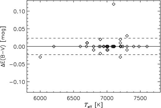
The differences between the E(B − V) values derived from interstellar maps and the sodium Na D2 lines. The dashed lines show 1σ level.
The E(B − V) values and atmospheric parameters derived from the photometric indices and SED analysis.
| HD | E(B − V) | E(B − V) | Teff | log g | Teff | log g | Teff | Teff | Teff | Teff |
|---|---|---|---|---|---|---|---|---|---|---|
| number | Map | |$^{NaD_2}$| | uvbyβ | uvbyβ | Geneva | Geneva | UBV | 2MASS | Averagea | SED |
| (mag) | (mag) | (K) | (dex) | (K) | (dex) | (K) | (K) | (K) | (K) | |
| ± 95 | ± 0.10 | ± 125 | ± 0.11 | ± 170 | ± 80 | ± 245 | ||||
| 009365 | 0.01 | 0.00 | 7050 | 4.05 | 7200 | 6940 | 7060 | 7280 ± 190 | ||
| 019655 | 0.03 | 0.03 | 6950 | 3.96 | 6850 | 4.06 | 7110 | 7130 | 7010 | 6800 ± 150 |
| 021788 | 0.02 | 0.02 | 6530 | 3.46 | 6930 | 6680 | 6750 | 6860 ± 200 | ||
| 022702 | 0.03 | 0.03 | 6940 | 4.28 | 7050 | 7040 | 7010 | 6800 ± 100 | ||
| 023005 | 0.00 | 0.00 | 7030 | 3.88 | 6920 | 4.07 | 6940 | 6870 | 6940 | 6970 ± 120 |
| 023585 | 0.03 | 0.00 | 7530 | 4.31 | 7080 | 4.26 | 7180 | 7220 | 7250 | 6990 ± 170 |
| 026298 | 0.01 | 0.00 | 6730 | 4.11 | 6720 | 4.38 | 6910 | 6820 | 6790 | 6670 ± 130 |
| 033204 | 0.00 | 0.00 | 7650 | 4.11 | 7210 | 4.04 | 7330 | 7510 | 7425 | 7170 ± 150 |
| 046304 | 0.00 | 0.00 | 7380 | 3.88 | 7370 | 4.25 | 7430 | 7270 | 7360 | 7150 ± 150 |
| 063436 | 0.00 | 0.00 | 7350 | 4.44 | 6890 | 7090 | 7110 | 7280 ± 110 | ||
| 089781 | 0.04 | 0.00 | 7090 | 4.03 | 7050 | 7180 | 7110 | 7060 ± 130 | ||
| 099267 | 0.00 | 0.00 | 7050 | 4.01 | 7110 | 7030 | 7060 | 7060 ± 100 | ||
| 099329 | 0.00 | 0.00 | 7070 | 4.02 | 6940 | 4.23 | 7000 | 6940 | 6990 | 6870 ± 100 |
| 104860 | 0.03 | 0.00 | 5920 | 4.65 | 6000 | 5970 | 5960 | 6160 ± 110 | ||
| 106103 | 0.00 | 0.00 | 6710 | 4.45 | 6650 | 4.55 | 6690 | 6590 | 6660 | 6530 ± 100 |
| 107192 | 0.00 | 0.01 | 7090 | 4.26 | 7010 | 4.46 | 6910 | 6830 | 6960 | 7050 ± 160 |
| 109032 | 0.00 | 0.00 | 7180 | 4.31 | 7070 | 7030 | 7090 | 7040 ± 120 | ||
| 109799 | 0.00 | 0.00 | 7020 | 4.07 | 6940 | 4.33 | 7060 | 6830 | 6960 | 6870 ± 150 |
| 109838 | 0.02 | 0.00 | 7060 | 4.12 | 7250 | 7170 | 7160 | 7000 ± 250 | ||
| 110379 | 0.00 | 0.00 | 7240 | 4.06 | 6850 | 5720 | 6600 | 6730 ± 300 | ||
| 112429 | 0.00 | 0.00 | 7210 | 4.20 | 7200 | 4.40 | 7280 | 7030 | 7180 | 7010 ± 100 |
| 118388 | 0.01 | 0.01 | 6590 | 6230 | 6410 | 6540 ± 250 | ||||
| 126516 | 0.01 | 0.00 | 6630 | 4.38 | 6540 | 6350 | 6510 | 6520 ± 250 | ||
| 130173 | 0.00 | 0.01 | 6430 | 3.77 | 6610 | 6450 | 6500 | 6570 ± 200 | ||
| 155154 | 0.00 | 0.00 | 7170 | 4.04 | 7160 | 7130 | 7150 | 7080 ± 140 | ||
| 165645 | 0.00 | 0.00 | 7320 | 4.02 | 7440 | 7220 | 7330 | 7160 ± 160 | ||
| 169577 | 0.15 | 0.03 | 7050 | 4.24 | 7400 | 7350 | 7270 | 7190 ± 300 | ||
| 187353 | 0.00 | 0.03 | 7020 | 4.10 | 7000 | 7040 | 7020 | 7040 ± 300 | ||
| 206043 | 0.00 | 0.00 | 7180 | 4.05 | 7110 | 6830 | 7040 | 7200 ± 120 | ||
| 075202 | 0.00 | 0.01 | 8180 | 4.06 | 7840 | 4.21 | 7890 | 7680 | 7900 | 8130 ± 250 |
| 091201 | 0.01 | 0.01 | 7070 | 4.10 | 7090 | 6980 | 7050 | 6960 ± 350 | ||
| 103257 | 0.00 | 0.00 | 6890 | 3.90 | 7100 | 6940 | 6980 | 6960 ± 100 | ||
| 113357 | 0.01 | 0.01 | 7150 | 4.26 | 7100 | 6900 | 7050 | 6930 ± 300 | ||
| 133803 | 0.01 | 0.02 | 7140 | 4.12 | 6940 | 7030 | 7040 | 7000 ± 150 | ||
| 137785 | 0.00 | 0.00 | 7110 | 4.06 | 7050 | 6820 | 7000 | 6900 ± 250 | ||
| 149989 | 0.00 | 0.00 | 7180 | 4.08 | 7070 | 4.43 | 7210 | 7040 | 7120 | 7000 ± 100 |
| 188032 | 0.00 | 0.00 | 7230 | 4.20 | 7080 | 4.47 | 7200 | 7130 | 7160 | 6900 ± 200 |
| 197451 | 0.01 | 0.02 | 7370 | 3.93 | 6900 | 7130 | 7130 | 7050 ± 300 | ||
| 206481 | 0.00 | 0.00 | 7150 | 4.24 | 7010 | 4.52 | 6950 | 7040 | 7040 | 6760 ± 150 |
| 224288 | 0.00 | 0.00 | 7140 | 4.22 | 6940 | 4.40 | 7040 | 6810 | 6980 | 6770 ± 120 |
| 112934 | 0.00 | 0.00 | 7120 | 4.14 | 7150 | 4.56 | 7220 | 7080 | 7140 | 6900 ± 160 |
| 115466 | 0.00 | 0.00 | 6970 | 3.93 | 6960 | 6940 | 6960 | 7200 ± 130 | ||
| 124248 | 0.00 | 0.00 | 7220 | 4.16 | 7220 | 7100 | 7180 | 7400 ± 130 | ||
| 171834 | 0.00 | 0.00 | 6720 | 4.03 | 6750 | 4.37 | 6950 | 6680 | 6780 | 6780 ± 200 |
| 172416 | 0.00 | 0.00 | 6590 | 4.13 | 6290 | 3.68 | 6400 | 6200 | 6370 | 6445 ± 100 |
| 175337 | 0.00 | 0.00 | 7090 | 4.14 | 6900 | 7090 | 7030 | 7290 ± 160 | ||
| 187028 | 0.00 | 0.00 | 7270 | 4.34 | 7090 | 4.47 | 7240 | 7010 | 7150 | 6920 ± 150 |
| 209295 | 0.00 | 0.00 | 7510 | 4.97 | 7470 | 4.25 | 7470 | 7480 | 7480 | 7110 ± 220 |
| 216910 | 0.00 | 0.00 | 7070 | 4.07 | 6930 | 4.27 | 6950 | 6880 | 6960 | 7390 ± 150 |
| 224638 | 0.00 | 0.00 | 7140 | 4.06 | 7160 | 6960 | 7090 | 6940 ± 200 | ||
| 224945 | 0.00 | 0.00 | 7268 | 7238 | 7250 | 7300 ± 160 | ||||
| 041448 | 0.00 | 0.00 | 7240 | 4.13 | 7170 | 7180 | 7200 | 7290 ± 150 |
aRepresents the average values of effective temperature obtained from different photometric systems.
4.1 Photometric parameters
The effective temperatures Teff and surface gravities log g of our targets were determined from photometric indices. These photometric parameters serve as input values for further analysis. We used uvbyβ Strömgren, Johnson, Geneva and 2MASS photometric data gathered from the General Catalogue of Photometric Data (Mermilliod, Mermilliod & Hauck 1997) and the 2MASS catalogue (Cutri et al. 2003).
For 49 stars, the atmospheric parameters Teff and log g were estimated from the uvbyβ system. These parameters were acquired using the method of Moon & Dworetsky (1985), based on the V, (b − y), m1, c1 and β indices.
For 23 stars, Geneva photometry was used to derive the Teff and log g values. The calculations were performed using the Künzli et al. (1997) calibration based on the B2 − V1, d and m2 indices.
Johnson (B − V) colour indices were used to determine the Teff of all studied stars. We applied the (B − V) colour–temperature relation given by Sekiguchi & Fukugita (2000). For calculations of Teff values, log g = 4.0 and solar metallicities were assumed.
Finally, Teff values of the stars were derived from the 2MASS photometry (Masana, Jordi & Ribas 2006), using (V − K) index. In the calculations, we assumed solar metallicity ([m/H] = 0.0) and log g = 4.0 for all the stars.
The results obtained with all these methods are listed in Table 3. Uncertainties of the calculated Teff and log g were estimated taking into account errors of photometric indices, reddening (0.02 mag, as discussed before), metallicity (0.1 dex), and surface gravity (0.1 dex), if it was necessary to assume this last parameter. Finally, we derived the average uncertainties of Teff and log g for each system (see Table 3). The average effective temperatures were calculated using the results from all considered photometric systems. In Fig. 2, these values are compared with individual results for each photometric system. The dashed lines represent the standard deviations of differences between the average temperatures and values from a given photometric system. These standard deviations are equal 125, 94, 96 and 140 K for uvbyβ, Geneva, Johnson and 2MASS systems, respectively. As can be seen in Fig. 2, in most cases the obtained effective temperatures are consistent with the average values. In the case of uvbyβ, the biggest difference was derived for HD 110379. This star is a binary system member, and its photometric colours can be influenced by the light from the second component.
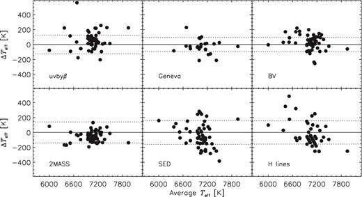
The differences between the average photometric effective temperatures and the Teff obtained from photometric methods, SED and hydrogen lines. The dashed lines show 1σ levels.
Additionally, the log g values obtained from the uvbyβ and Geneva indices were compared with each other. The average log g value for the uvbyβ system is 4.08 dex while for the Geneva system, it reaches 4.32 dex. As can be inferred from these average values, surface gravities from uvbyβ are in general slightly lower than the Geneva ones.
4.2 Effective temperature from SED
Stellar parameters can be estimated from the SED of a star. SEDs have to be constructed from spectrophotometry collected in different wavelengths, preferably from ultraviolet until infrared. Different parts of SED are sensitive to different stellar parameters. We used SEDs to obtain Teff values, using the code written by Dr Shulyak (private information). This code automatically searches for spectrophotometric observations from different data bases. Several data bases are available with the code, e.g. Adelman et al. (1989), Breger (1976), Alekseeva et al. (1996), Burnashev (1985) and Glushneva et al. (1992) covering the near-UV, visual, and near-IR wavelengths. The code can additionally use data from the Space Telescope Imaging Spectrograph (STIS, Hubble Space Telescope; Woodgate et al. 1998), the International Ultraviolet Explorer (IUE; Wamsteker et al. 2000), and the Ultraviolet Sky Survey Telescope (TD1; Boksenberg et al. 1973; Thompson et al. 1978). These archives cover the ultraviolet part of SED. The code allows also to input indices manually, if necessary.
In this study, we generally used the photometric colours of the uvbyβ, Geneva, Johnson, and 2MASS systems and the ultraviolet TD1 observations as input values. SEDs constructed from these observed spectrophotometric measurements were compared with theoretical energy distributions, calculated from the Kurucz's atmospheric models (atlas9 code; Kurucz 1993). In these calculations, the solar metallicity ([m/H] = 0) and the log g value of 4.0 dex were assumed. The obtained Teff values and their uncertainties are listed in Table 3. The average error is about 110 K. Differences between the obtained SED Teff values and the average photometric values are shown in Fig. 2. In the figure dashed lines represent standard deviations of 160 K. As can be seen from Fig. 2, the highest difference was derived for HD 209295. This can be caused by the membership of this star to a binary system.
5 SPECTROSCOPIC ANALYSIS
In this section, the analysis of high-resolution and high S/N spectra is presented. Atmospheric parameters were derived from the analysis of hydrogen and metal lines. All the necessary atmospheric models were calculated with the atlas9 code (Kurucz 1993) that generates hydrostatic, plane-parallel and line-blanketed local thermodynamic equilibrium models. The synthetic spectra were obtained with the synthe code (Kurucz & Avrett 1981).
5.1 Analysis of hydrogen lines
The hydrogen lines analysis was applied to obtain the Teff values of all stars. During the analysis of Balmer lines, the log g values were assumed to be 4.0 dex. Additionally, the solar metallicity and vsin i values were fixed during the analysis. The initial values of vsin i were taken from the approximate fitting of the synthetic spectra to the observed metal lines. The analysis was performed taking into account the Hβ, Hγ and Hδ lines. The method proposed by Catanzaro, Leone & Dall (2004) was applied. Initial Teff values were taken from previous calculations, including photometric and the SED Teff results. The final effective temperatures were derived minimizing the differences between synthetic and observed spectra. As an example, the result of the analysis for HD 23005 is shown in Fig. 3. As can be seen, the observed hydrogen lines fit quite well with the synthetic spectra. The small deviations in the core of the lines are caused by the incorrect models, which are not able to explain Balmer line cores. The effective temperatures derived from the hydrogen lines and their uncertainties are listed in Table 4. These uncertainties were determined taking into account uncertainties resulting from quality of the spectra (S/N) and assumed values of log g, [m/H] and vsin i. As known, the hydrogen lines are not sensitive to log g in the temperature range of γ Dor stars. Because of this, the log g parameter has no significant effect on Teff values in our analysis (Smalley et al. 2002; Smalley 2005). The obtained uncertainties are in the range of ∼ 150–260 K.
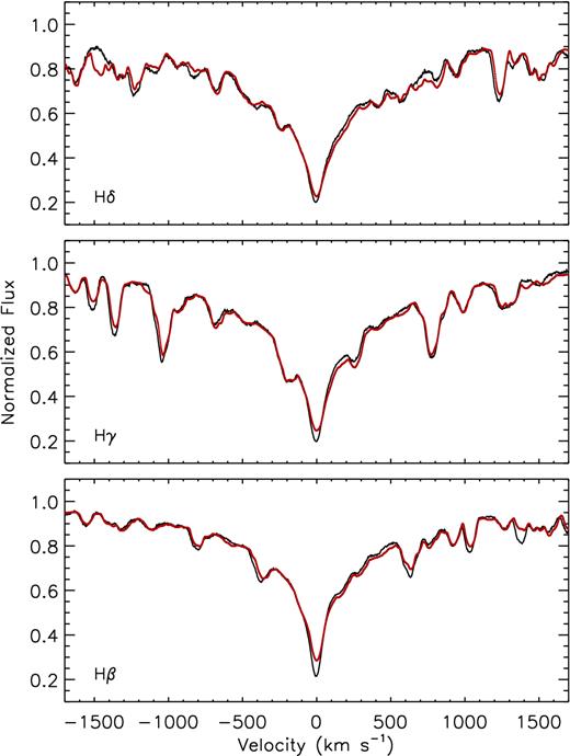
The observed Balmer lines (black lines) and the synthetic spectra (red lines) for HD 23005.
Atmospheric parameters obtained from the hydrogen and iron lines analysis. Previously determined spectroscopic atmospheric parameters: HD23585: Teff = 7440 K, log g = 4.29, ξ = 3.0 km s−1 (Gray, Graham & Hoyt 2001) HD26298: Teff = 6790 ± 200 K, log g = 3.95 ± 0.22, ξ = 1.5 ± 0.5 km s−1, HD110379: Teff = 7140 ± 160 K, log g = 4.21 ± 0.02, ξ = 1.5 ± 0.4 km s−1, HD126516: Teff = 6590 ± 120 K, log g = 4.01 ± 0.15, ξ = 1.9 ± 0.3 km s−1 (Bruntt et al. 2008) HD33204: Teff = 7646 K, log g = 4.11, ξ = 3.4 (Varenne & Monier 1999) HD46304: Teff = 7048 ± 16 K, HD63436: Teff = 6970 K, log g = 4.14, HD106103: Teff = 6610 K (Muñoz Bermejo et al. 2013) HD99329: Teff = 6990 K, HD112934: Teff = 7035 K, HD209295: Teff = 7392 K (Ammler-von Eiff & Reiners 2012) H109799: Teff = 6926 ± 26 K (King & Schuler 2005).
| HD | TeffHlines | TeffFelines | log gFelines | ξ | vsin i | log ϵ (Fe) |
|---|---|---|---|---|---|---|
| number | (K) | (K) | (dex) | (km s−1) | (km s−1) | (dex) |
| 009365 | 7000 ± 170 | 7200 ± 100 | 3.9 ± 0.1 | 2.7 ± 0.2 | 77 ± 1 | 7.39 ± 0.22 |
| 019655 | 7000 ± 210 | 7100 ± 100 | 4.1 ± 0.3 | 2.8 ± 0.4 | 222 ± 5 | 7.32 ± 0.23 |
| 021788 | 6600 ± 140 | 6700 ± 100 | 4.1 ± 0.2 | 2.2 ± 0.1 | 13 ± 1 | 7.26 ± 0.21 |
| 022702 | 7000 ± 190 | 7200 ± 200 | 4.2 ± 0.2 | 2.5 ± 0.3 | 146 ± 2 | 7.40 ± 0.24 |
| 023005 | 7100 ± 150 | 7000 ± 100 | 3.9 ± 0.1 | 2.4 ± 0.1 | 48 ± 1 | 7.61 ± 0.21 |
| 023585 | 7300 ± 250 | 7200 ± 200 | 4.1 ± 0.2 | 2.8 ± 0.3 | 113 ± 3 | 7.40 ± 0.24 |
| 026298 | 6700 ± 150 | 6700 ± 100 | 4.1 ± 0.1 | 2.0 ± 0.2 | 53 ± 2 | 7.20 ± 0.22 |
| 033204 | 7500 ± 230 | 7600 ± 200 | 4.0 ± 0.1 | 3.1 ± 0.1 | 36 ± 2 | 7.97 ± 0.26 |
| 046304 | 7300 ± 260 | 7400 ± 100 | 4.0 ± 0.1 | 3.0 ± 0.4 | 242 ± 12 | 7.31 ± 0.27 |
| 063436 | 7000 ± 170 | 7000 ± 100 | 3.9 ± 0.1 | 1.7 ± 0.2 | 70 ± 1 | 7.45 ± 0.22 |
| 089781 | 7000 ± 180 | 7200 ± 100 | 4.2 ± 0.2 | 1.3 ± 0.2 | 120 ± 3 | 7.45 ± 0.23 |
| 099267 | 7000 ± 170 | 7000 ± 100 | 4.2 ± 0.2 | 2.9 ± 0.3 | 100 ± 2 | 7.46 ± 0.23 |
| 099329 | 6900 ± 200 | 7100 ± 200 | 4.1 ± 0.2 | 2.6 ± 0.3 | 142 ± 2 | 7.49 ± 0.24 |
| 104860 | 6100 ± 140 | 6000 ± 100 | 4.4 ± 0.2 | 1.9 ± 0.1 | 16 ± 2 | 7.34 ± 0.21 |
| 106103 | 6600 ± 150 | 6700 ± 100 | 4.1 ± 0.2 | 1.3 ± 0.1 | 21 ± 1 | 7.40 ± 0.21 |
| 107192 | 6900 ± 160 | 7000 ± 100 | 3.9 ± 0.2 | 2.8 ± 0.2 | 69 ± 1 | 7.32 ± 0.22 |
| 109032 | 7000 ± 170 | 7000 ± 100 | 4.2 ± 0.2 | 2.6 ± 0.2 | 100 ± 1 | 7.42 ± 0.22 |
| 109799 | 6900 ± 140 | 7000 ± 100 | 4.0 ± 0.1 | 1.8 ± 0.1 | 39 ± 2 | 7.51 ± 0.21 |
| 109838 | 7000 ± 140 | 6900 ± 100 | 4.2 ± 0.1 | 1.5 ± 0.1 | 13 ± 1 | 7.46 ± 0.21 |
| 110379 | 7000 ± 150 | 7100 ± 100 | 4.1 ± 0.1 | 1.8 ± 0.2 | 34 ± 6 | 7.37 ± 0.21 |
| 112429 | 7100 ± 170 | 7200 ± 100 | 3.9 ± 0.2 | 3.0 ± 0.2 | 120 ± 3 | 7.29 ± 0.23 |
| 118388 | 6800 ± 170 | 6700 ± 100 | 4.1 ± 0.2 | 1.9 ± 0.2 | 121 ± 8 | 7.27 ± 0.22 |
| 126516 | 7000 ± 140 | 6800 ± 200 | 4.2 ± 0.2 | 1.5 ± 0.2 | 5 ± 1 | 7.50 ± 0.23 |
| 130173 | 6700 ± 160 | 6800 ± 200 | 4.0 ± 0.2 | 2.2 ± 0.2 | 62 ± 3 | 7.28 ± 0.23 |
| 155154 | 7100 ± 200 | 7000 ± 100 | 4.0 ± 0.2 | 3.0 ± 0.3 | 183 ± 6 | 7.30 ± 0.22 |
| 165645 | 7200 ± 180 | 7300 ± 200 | 4.1 ± 0.1 | 3.2 ± 0.2 | 152 ± 4 | 7.36 ± 0.28 |
| 169577 | 7000 ± 160 | 7100 ± 200 | 4.2 ± 0.1 | 1.8 ± 0.2 | 62 ± 4 | 7.79 ± 0.23 |
| 187353 | 7300 ± 230 | 7200 ± 100 | 4.1 ± 0.1 | 1.7 ± 0.1 | 35 ± 2 | 7.36 ± 0.22 |
| 206043 | 7200 ± 190 | 7200 ± 200 | 4.0 ± 0.2 | 2.5 ± 0.2 | 135 ± 5 | 7.50 ± 0.23 |
| 075202 | 7700 ± 260 | 7900 ± 200 | 4.2 ± 0.2 | 0.4 ± 0.2 | 104 ± 2 | 7.51 ± 0.26 |
| 091201 | 7100 ± 150 | 7100 ± 100 | 3.8 ± 0.2 | 2.3 ± 0.1 | 50 ± 1 | 7.50 ± 0.18 |
| 103257 | 6900 ± 160 | 7100 ± 200 | 4.0 ± 0.2 | 2.3 ± 0.2 | 70 ± 2 | 7.31 ± 0.20 |
| 113357 | 7000 ± 160 | 7100 ± 100 | 4.1 ± 0.1 | 2.9 ± 0.2 | 67 ± 1 | 7.28 ± 0.19 |
| 133803 | 7000 ± 170 | 7000 ± 100 | 4.2 ± 0.3 | 2.2 ± 0.2 | 92 ± 2 | 7.37 ± 0.18 |
| 137785 | 7000 ± 170 | 6900 ± 100 | 3.8 ± 0.2 | 2.8 ± 0.2 | 109 ± 3 | 7.16 ± 0.18 |
| 149989 | 7000 ± 190 | 7100 ± 100 | 4.0 ± 0.2 | 2.8 ± 0.2 | 140 ± 6 | 7.09 ± 0.19 |
| 188032 | 7000 ± 160 | 7100 ± 100 | 4.0 ± 0.1 | 2.5 ± 0.2 | 54 ± 2 | 7.34 ± 0.18 |
| 197451 | 7400 ± 230 | 7300 ± 200 | 4.0 ± 0.1 | 3.1 ± 0.2 | 26 ± 3 | 7.73 ± 0.22 |
| 206481 | 6900 ± 170 | 6900 ± 100 | 4.1 ± 0.2 | 1.5 ± 0.2 | 86 ± 2 | 7.36 ± 0.18 |
| 224288 | 7100 ± 150 | 7100 ± 200 | 3.9 ± 0.1 | 2.2 ± 0.2 | 48 ± 2 | 7.39 ± 0.19 |
| 112934 | 7000 ± 170 | 7100 ± 100 | 3.9 ± 0.2 | 2.4 ± 0.2 | 75 ± 2 | 7.03 ± 0.22 |
| 115466 | 6800 ± 150 | 7100 ± 100 | 4.0 ± 0.2 | 2.0 ± 0.2 | 40 ± 3 | 7.56 ± 0.20 |
| 124248 | 7000 ± 150 | 7100 ± 100 | 4.1 ± 0.1 | 1.7 ± 0.2 | 50 ± 3 | 7.37 ± 0.20 |
| 171834 | 6700 ± 170 | 7000 ± 100 | 4.0 ± 0.2 | 2.7 ± 0.2 | 72 ± 2 | 7.40 ± 0.21 |
| 172416 | 6400 ± 150 | 6400 ± 100 | 3.9 ± 0.1 | 1.9 ± 0.2 | 55 ± 3 | 7.41 ± 0.20 |
| 175337 | 6900 ± 150 | 7100 ± 100 | 4.0 ± 0.1 | 1.7 ± 0.1 | 38 ± 2 | 7.73 ± 0.19 |
| 187028 | 6900 ± 170 | 7300 ± 200 | 4.5 ± 0.2 | 2.3 ± 0.3 | 87 ± 3 | 7.23 ± 0.23 |
| 209295 | 7400 ± 170 | 7300 ± 100 | 4.2 ± 0.1 | 2.3 ± 0.2 | 89 ± 5 | 7.07 ± 0.21 |
| 216910 | 6900 ± 180 | 7100 ± 100 | 4.3 ± 0.2 | 2.1 ± 0.2 | 95 ± 4 | 7.66 ± 0.21 |
| 224638 | 6900 ± 140 | 7000 ± 100 | 4.0 ± 0.1 | 1.5 ± 0.2 | 29 ± 7 | 7.39 ± 0.20 |
| 224945 | 7000 ± 150 | 7300 ± 100 | 4.2 ± 0.1 | 2.3 ± 0.2 | 58 ± 2 | 7.39 ± 0.23 |
| 041448 | 7300 ± 170 | 7200 ± 100 | 4.1 ± 0.2 | 2.8 ± 0.2 | 104 ± 3 | 7.35 ± 0.18 |
In Fig. 2, the obtained values are compared with the average Teff calculated from photometric indices. Standard deviation of these differences is about 200 K, and is shown by the dashed lines in Fig. 2. In Fig. 4, Teff parameters from hydrogen lines are compared with the results of SED and iron lines analysis. The results are consistent within the error bars. Standard deviations and average values of these distributions are given in Fig. 4.
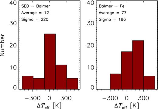
The distributions of differences between the effective temperatures determined from the hydrogen lines and SED analysis (left-hand panel) and from the hydrogen and Fe lines analysis (right-hand panel).
5.2 Atmospheric parameters from iron lines analysis
When Teff and log g values were determined from photometric methods, SEDs and hydrogen lines, the iron lines analysis was performed assuming previously determined parameters as inputs. The initial analysis of the stellar vsin i values, revealed slowly and fast rotating stars in our sample. High rotation velocity causes that most of the spectral lines are blended. To analyse such spectra and to determine atmospheric parameters (Teff, log g and microturbulent velocity ξ), the spectrum synthesis is the most appropriate method. To perform our analysis, we followed the same procedure as described in Niemczura et al. (2015). The values of Teff, log g and ξ were determined taking into account Fe i and Fe ii lines. Teff and ξ parameters are highly sensitive to the strength of the Fe i lines while the log g parameter is almost totally insensitive to it. The strength of the Fe ii lines is slightly affected by Teff and ξ, but depends considerably on the log g. Considering the mentioned dependence of the iron lines on atmospheric parameters, we first obtained ξ values by looking at the correlation between the Fe i lines depths and abundances. Secondly, Teff values were derived by checking the correlation between the excitation potential and the abundances calculated from individual Fe i lines. In both cases the correlations should be nearly zero, which means that for the proper atmospheric parameters of a star, the same iron abundance should be obtained from all iron lines. The surface gravity values were determined using the ionization balance of the Fe i and Fe ii lines.
In Fig. 5, we show the distributions of the derived iron abundances (left), excitation potentials versus Fe i abundances (middle) and Fe i lines depths versus abundances (right) for the star HD 126516. Additionally, two sets of the atmospheric parameters for which the iron abundances were calculated are shown. The upper panels show these relations for the wrong atmospheric parameters, whereas the lower panels demonstrate the right solution. As we expect that for the correct parameters all iron lines give the same iron abundance within the error bars, it is clear that the smallest correlations of line strength, excitation potential, and obtained abundances indicate the correct solution.
The distributions of the derived iron abundances, the Fe i abundances versus the excitation potential and the lines’ depths for HD 126516. The ‘i’ values illustrate an inclination of the fitted line. The first set of parameters (Teff = 7100 K, log g = 4.2, ξ = 3 km s−1) is incorrect (upper panels), while the second set (6800 K, 4.2 dex, 1.5 km s−1) is the right one (lower panels).
The derived values for Teff, log g and ξ together with their uncertainties are given in Table 4. The errors of the analysed parameters were obtained taking into account the effect of other parameters on the considered one. The lowest errors of 100 K for Teff, 0.1 dex for log g, and 0.1 km s−1 for ξ result from the steps adopted in the calculated stellar atmospheric models and synthetic spectra.
5.3 Abundances analysis
After the determination of Teff, log g and ξ, chemical abundance analysis was carried out. In the first step, the spectra of each star were divided into the parts which widths depend mainly on vsin i. For slowly rotating stars, parts covering only one or a few blended spectral features were selected. For moderate and fast rotating stars broader spectral ranges, including blends of many lines, were used. All parts were re-normalized by comparison with theoretical spectra, if necessary. Then the line identification for selected regions was performed using the line list of Kurucz3 (Kurucz & Bell 1995) taking into account only these elements that are most important in the given region. The abundance analysis was carried out by the spectrum synthesis method, which allowed us to determine chemical abundances and vsin i values at the same time. We used the classical least square method. Minimum differences between the observed and synthetic spectra indicate the final solution. After carrying out calculations for each spectral part of a given star, the average values of vsin i and chemical abundances were derived. The results are presented in Table 4 (vsin i and iron abundances) and Table 5 (chemical abundances and standard deviations).
The average abundances and standard deviations of individual elements of the stars. Number of the analysed parts is given in the brackets. The full table is available in the electronic form.
| Elements | HD 9565 | HD 19655 | HD 21788 | HD 22702 | HD 23005 |
|---|---|---|---|---|---|
| (Atomic number) | |||||
| C (6) | 8.48 ± 0.15 (7) | 8.34 ± 0.24 (2) | 8.52 ± 0.21 (19) | 8.65 ± 0.01 (3) | 8.11 ± 0.27 (8) |
| N (7) | 8.61 ± 0.19 (1) | ||||
| O (8) | 8.57 ± 0.19 (2) | ||||
| Na (11) | 5.62 ± 0.14 (2) | 6.65 ± 0.24 (1) | 6.08 ± 0.05 (4) | 6.25 ± 0.13 (1) | 6.47 ± 0.28(2) |
| Mg (12) | 7.64 ± 0.09 (8) | 7.57 ± 0.01 (4) | 7.51 ± 0.22 (11) | 7.69 ± 0.15 (5) | 7.86 ± 0.20 (8) |
| Si (14) | 7.21 ± 0.30 (16) | 6.48 ± 0.35 (4) | 7.09 ± 0.43 (40) | 6.94 ± 0.32 (6) | 7.15 ± 0.35 (21) |
| S (16) | 7.29 ± 0.14 (2) | 7.20 ± 0.12 (8) | 7.41 ± 0.28 (2) | ||
| Ca (20) | 6.48 ± 0.19 (19) | 6.32 ± 0.16 (4) | 6.38 ± 0.20 (32) | 6.29 ± 0.06 (4) | 7.01 ± 0.30 (27) |
| Sc (21) | 2.94 ± 0.12 (10) | 3.44 ± 0.24 (5) | 3.20 ± 0.07 (8) | 3.52 ± 0.13 (2) | 3.47 ± 0.30 (12) |
| Ti (22) | 4.94 ± 0.11 (23) | 4.94 ± 0.04 (7) | 4.95 ± 0.23 (92) | 4.85 ± 0.16 (9) | 4.93 ± 0.23 (36) |
| V (23) | 4.94 ± 0.14 (2) | 3.88 ± 0.21 (10) | 4.26 ± 0.50 (4) | ||
| Cr (24) | 5.56 ± 0.07 (15) | 5.59 ± 0.15 (7) | 5.48 ± 0.23 (85) | 5.57 ± 0.06 (3) | 5.64 ± 0.44 (39) |
| Mn (25) | 5.03 ± 0.33 (8) | 4.85 ± 0.24 (1) | 4.94 ± 0.25 (21) | 5.17 ± 0.13 (2) | 5.30 ± 0.19 (8) |
| Fe (26) | 7.39 ± 0.06 (40) | 7.32 ± 0.04 (9) | 7.26 ± 0.14 (299) | 7.40 ± 0.13 (15) | 7.61 ± 0.12 (127 |
| Co (27) | 4.40 ± 0.21 (6) | 5.37 ± 0.28 (4) | |||
| Ni (28) | 6.13 ± 0.08 (16) | 6.03 ± 0.08 (3) | 5.94 ± 0.16 (88) | 6.20 ± 0.13 (2) | 6.41 ± 0.20 (23) |
| Cu (29) | 3.56 ± 0.14 (2) | 3.52 ± 0.24 (3) | 4.11 ± 0.28 (1) | ||
| Zn (30) | 4.18 ± 0.19 (1) | ||||
| Sr (38) | 3.06 ± 0.14 (1) | 3.73 ± 0.19 (1) | 2.39 ± 0.13 (1) | 3.92 ± 0.28 (2) | |
| Y (39) | 2.31 ± 0.13 (4) | 1.92 ± 0.24 (2) | 2.34 ± 0.10 (10) | 2.61 ± 0.13 (2) | 3.17 ± 0.23 (6) |
| Zr (40) | 2.43 ± 0.14 (2) | 2.62 ± 0.24 (1) | 2.92 ± 0.21 (12) | 2.80 ± 0.13 (2) | 3.16 ± 0.28 (2) |
| Ba (56) | 2.27 ± 0.16 (3) | 2.98 ± 0.24 (2) | 2.95 ± 0.15 (4) | 2.57 ± 0.13 (2) | 2.77 ± 0.34 (3) |
| La (57) | 1.56 ± 0.19 (2) | 2.11 ± 0.28 (2) | |||
| Ce (58) | 1.79 ± 0.09 (10) | 1.84 ± 0.28 (2) | |||
| Pr (59) | 0.33 ± 0.19 (1) | ||||
| Nd (60) | 1.54 ± 0.20 (19) | 1.59 ± 0.28 (2) | |||
| Sm (62) | 1.54 ± 0.19 (1) |
The uncertainties of chemical elements given in Table 5 are standard deviations. The real errors of the elements include the effects of assumptions adopted to build the model of the atmosphere and uncertainties of atmospheric parameters (Teff, log g, ξ). The assumptions like local thermodynamical equilibrium, plane-parallel geometry, and hydrostatic equilibrium were adopted in calculations of atmospheric models and synthetic spectra. They introduce the error of about 0.1 dex for calculated chemical abundances (Mashonkina 2011). Other important factors are used atomic data, analysed wavelength range, quality of the data (resolution, S/N), and normalization of the spectra.
To find out the effect of resolution and S/N ratio on the values of the obtained chemical abundances, we selected three stars observed by different instruments with different or similar S/N ratios. First of these stars (HD 109799) was observed by FIES (R = 67 000) and HARPS (R = 80 000) spectrographs. Obtained spectra have almost the same S/N ratios (∼ 310). We performed the standard analysis of both spectra and obtained a 0.07 dex difference in iron abundance. For the second star (HD 23005), the spectra were collected by FIES (R = 67 000) with S/N = 300 and by HERMES (R = 85 000) with S/N = 180 ratio. According to the S/N ratio and the resolving power of these spectra, both spectra have approximately the same quality. In case of this star, we got the difference in iron abundance of about 0.02 dex. For the third star (HD 133803), we have spectra from HARPS (R = 80 000) with S/N = 310 ratio and from HERMES (R = 85 000) with S/N = 170 ratio. The spectra have nearly the same resolution but different S/N values. When we compared the obtained abundances of iron, 0.13 dex difference was derived. These calculations show, that the resolving power does not have significant influence on abundance determinations in our spectral analysis, as all data were taken by high-resolution instruments. On the other hand, the S/N ratio has more important effect.
We also checked the possible influence of quality of the spectrum on atmospheric parameters determination. The stars were observed by spectrographs with resolving powers equal 67 000, 80 000 and 85 000. Collected spectra have S/N more than 100, often S/N more than 150. We can state that the latter value is the recommended one to be used in the abundance analyses, since the improvements obtained with higher S/N spectra could not be justified by larger investment of observing time. However, we found no substantial effect of the resolving power and S/N ratio on atmospheric parameters. Similar results were also obtained by Ryabchikova et al. (2016).
The influence of uncertainties of atmospheric parameters and vsin i on chemical abundances was examined as well. We obtained that 100 K uncertainty of Teff causes the change in element abundance of less than 0.1 dex. This value increases with increasing Teff. On the other hand, the 0.1 dex error of log g changes the chemical abundances of about 0.04 dex or less. Additionally, we found that for stars in our effective temperature range, 0.1 km s−1 uncertainty in ξ value changes the element abundance of less than 0.1 dex. The significant influence on the determined abundances can obtain the uncertainty of the vsin i value. To examine this effect, we checked the abundance differences caused by changes of vsin i in the range from ∼ 5 to 15 km s−1, depending on the projected rotation velocity of the star. Higher value of vsin i implies higher value of its uncertainty. These uncertainties cause differences in abundances ranging from 0.1 to 0.2 dex. The effect increases with increasing projected rotational velocity. Finally, we considered all mentioned uncertainties to calculate the total error of chemical abundances. This value can be as high as 0.28 dex but for most cases it is about 0.20 dex. These errors were also calculated by Niemczura et al. (2015) for hotter stars. They found these values less than 0.20 dex for their targets. The total errors of iron abundances are given in Table 4.
5.4 Discussion of the results
Effective temperatures
The stellar Teff parameters were determined by various methods. The final values were obtained from the iron lines analysis. As can be seen in the left-hand panel of Fig. 6, the Teff range for the full sample is between 6000 and 7900 K, while bona-fide γ Dor stars have effective temperatures from 7100 to 7300 K. This range is in agreement with the results of the previous studies (Handler & Shobbrook 2002; Bruntt et al. 2008; Tkachenko et al. 2012, 2013a; Van Reeth et al. 2015).
The atmospheric parameters distribution of γ Dor stars. Light blue histograms show the distributions for the full sample while the histograms of the dark blue slant lines illustrates bona-fide γ Dor stars.
For 12 stars in our survey, the spectroscopic Teff values were determined previously. Information about these stars is given in Table 4. We compared our Teff values with the ones given in the literature for these objects. It turned out that effective temperatures of the mentioned stars are in agreement within an error of 200 K. Only in the case of HD 46304, the difference between Teff obtained here and that given by Muñoz Bermejo, Asensio Ramos & Allende Prieto (2013) reaches 400 K. This difference can be explained by the effect of stellar membership in the visual binary system and differences in methods of an atmospheric parameter analysis.
Surface gravities
The log g values were determined from the analysis of the Fe i and Fe ii lines (see Table 4). The distribution of the obtained log g values is given in the middle panel of Fig. 6. We derived surface gravities between 3.8 and 4.5 dex. Bruntt et al. (2008) obtained a log g range from 3.1 to 4.7 for bona-fide and candidate γ Dor stars while Van Reeth et al. (2015) found values between 3.3 and 4.5 for a sample of bona-fide γ Dor stars only. In our study, the average log g value amounts to 4.07 dex for the full sample and the average of 4.09 and 4.05 dex was found for bona-fide and candidate γ Dor stars, respectively. These values are slightly lower than those given in previous studies (4.16 dex by Bruntt et al. 2008; 4.10 dex by Van Reeth et al. 2015) what indicates that the stars analysed here are more evolved. From a comparison of our log g values with those found in the literature, we conclude that they agree within 0.2 dex.
Microturbulent velocities
The obtained microturbulent velocities range from 1.3 to 3.2 km s−1 (see right-hand panel of Fig. 6) for all stars except for HD 75202. This star is a candidate γ Dor star, listed in a catalogue of contact binary objects (Pribulla, Kreiner & Tremko 2003). The spectrum of HD 75202 can be affected by the other system member, which can influence the determined atmospheric parameters.
The range of ξ values is in agreement with the results of Landstreet et al. (2009), Gebran et al. (2014), and Niemczura et al. (2015). According to these studies, for effective temperatures between 7000 and 8000 K ξ values are mostly between 2 and 4 km s−1. The value of this parameter decreases for temperatures lower than ∼ 7000 K and higher than ∼ 8000 K. In the case of chemically peculiar Am stars, the ξ values are expected to be higher than for normal stars (Landstreet et al. 2009). We plotted the ξ parameter as a function of Teff in the right-hand panel of Fig. 7. As can be seen, the Am stars in our study show the same ξ values as non-chemically peculiar stars. A similar result for Am stars was obtained by Niemczura et al. (2015) and Smalley (2004). We also examined the variation of ξ values with surface gravity (left-hand panel of Fig. 7). The ξ values are lower with increasing values of log g. The same variations for F type stars were obtained by Gray et al. (2001).
The microturbulent velocities as a function of log g and Teff. The star symbols represent Am stars HD 33204 and HD 46304.
Van Reeth et al. (2015) found ξ values between 2 and 3.5 km s−1 for γ Dor stars, in agreement with our results. The small differences are due to the differences in the applied methods and adopted atomic data.
Projected rotational velocities
The vsin i values were derived during the analysis of the chemical abundances by the spectrum synthesis method. The range of the obtained projected rotational velocities is between 5 and 240 km s−1. The distribution of vsin i is shown in Fig. 8. The average vsin i value equal to 80 km s−1 was calculated taking into account all analysed stars. When considering bona-fide and candidate γ Dor stars separately, the average values are 97 and 63 km s−1, respectively. In the previous studies, this value obtained for bona-fide and candidate γ Dor stars equals 57 km s−1 (Henry & Fekel 2002, 2003; Fekel, Warner & Kaye 2003; Mathias et al. 2004; De Cat et al. 2006; Van Reeth et al. 2015). Van Reeth et al. (2015) gives the range from 12 to 204 km s−1 and the average value of 71 km s−1 for bona-fide γ Dor stars. All these values depend on the analysed sample of stars. However, both our results and Van Reeth et al. (2015) calculations suggest a great variation of projected rotational velocities of bona-fide γ Dor stars.
The rotational velocity distribution of the stars. The light blue histogram shows the distribution for the whole sample while the histogram of dark blue slant lines illustrates the distribution of bona-fide γ Dor stars.
In our study, most stars have high projected rotational velocities (vsin i > 100 km s−1). However, during the analysis we found some slowly rotating stars (HD 21788, HD 104860, HD 109838 and HD 126516) with vsin i < 15 km s−1. Not all chemically peculiar stars from our sample are slowly rotating stars. HD 33204 has vsin i value of 36 km s−1 while HD 46304 has vsin i = 242 km s−1. It has been shown that Am stars generally have smaller rotational velocities than normal stars (Abt & Hudson 1971).
Chemical abundances
The abundance pattern of γ Dor stars was examined in detail. The average relative abundance of bona-fide, candidate γ Dor, and non-pulsating F type stars were compared. The abundance distributions of four non-pulsating F type stars were taken from Niemczura et al. (2015), as the same analysis method is used in the current study. This comparison is demonstrated in Fig. 9. As can be seen, the abundances of both bona-fide and candidate γ Dor stars are close to the solar abundances.

The abundances of Am: stars were also examined in detail. As mentioned before, we identified two mild-Am stars, HD 33204 and HD 46304. We show abundance distributions of these stars in Fig. 10. A typical Am star exhibits overabundances of iron-peak elements and some heavy elements (Zn, Sr, Zr and Ba), but Ca and Sc abundances of these stars are underabundant (Gray & Corbally 2009). As can be seen in Fig. 10, the mild-Am stars in our study have nearly solar abundances of Ca and Sc elements. Only HD 33204 shows overabundances in some heavy elements typical for Am star. In the case of HD 46304, most of lines are blended due to high rotation velocity of the star. These blended lines cause difficulties in abundance calculations. The abundance differences between HD 46304 and a typical Am star can be caused by this effect. In the spectral classification process some stars were defined as metal-poor, mostly taking into account Mg, Mn and Fe lines (see Table 2). For these stars, the average abundance of Mg (7.57 dex) was found to be close to the solar abundance. However, the average abundances of Mn (5.13 dex) and Fe (7.27 dex) are slightly lower than the solar abundances. For some of our targets (HD 26298, HD 33204, HD 106103, HD 110379, and HD 126516) chemical abundances were already obtained before the present study. We compared our atmospheric parameters and abundance results with the literature values. Abundances of HD 33204 and HD 10613 were derived by Varenne & Monier (1999) and Fossati et al. (2008), respectively. In their work, similar methods for abundance analysis were used but different atomic data bases were adopted. For HD 33204 higher abundances of Sc, Mg and Y were obtained in the present study. Our result is consistent with the Am: type peculiarity of this star. For HD 106103 only the Y abundance is different. Abundances of HD 26298, HD 110379 and HD 126516 were derived by Bruntt et al. (2008) using the equivalent width method and the different atomic data base. In the case of these three stars, the marked differences were detected only for V and Ba abundances.
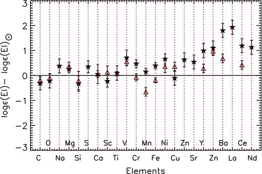
Chemical abundances of Am: stars compared with the solar values (Asplund et al. 2009). HD 33204 is represented by stars and HD 46304 by triangles.
Additionally, we checked the possible correlations of the element abundances with atmospheric parameters, i.e. Teff, log g and ξ. Similar as in Niemczura et al. (2015), no correlations were found. Moreover, the element abundances do not depend on vsin i. The same result was found by Fossati et al. (2008). However, Takeda et al. (2008) reported negative correlations between vsin i and C, O and Ca elements. Finally, we checked the relations between abundances of iron and other elements. Strong positive correlations were found for Mg, Si, Ca, Sc, Ti Cr, Ni, Y and Ba. Similar correlations between Fe abundances and iron-peak elements were found by Niemczura et al. (2015). On the other hand, a negative correlation was obtained between Fe and O abundances.
6 DISCUSSION AND CONCLUSIONS
This study presents a detailed analysis of the atmospheric parameters and chemical abundances of a sample bona-fide and candidate γ Dor stars. We analysed the high-resolution and high S/N spectra of 52 objects. The results of the spectral classifications show that the spectral types of γ Dor stars are between A7 and F9 and that their luminosity classes range from V to IV. During the spectral classifications process, two mild-Am stars, HD 33204 and HD 46304 were defined. Peculiarities of these stars were checked with the results of the detailed abundance analysis. Only for HD 33204 this peculiarity was confirmed. Because of the high rotation velocity of HD 46304, the peculiarity of this star could not be confirmed.
To determine the initial atmospheric parameters (Teff and log g), we used photometric indices, SEDs and hydrogen lines. The obtained Teff values were compared with each other. We found that effective temperatures from different methods are mostly in agreement. The final atmospheric parameters of the stars were derived from iron lines analysis using the spectrum synthesis method. The agreement between the new results obtained with our analysis and those previously available shows the robustness of the spectroscopic procedures adopted to analyse the chemical abundances of A-F stars.
For the whole sample, the obtained Teff values range from 6000 to 7900 K, while the obtained log g changes from 3.8 to 4.5 dex. This result corresponds with the obtained luminosity type of the stars. Additionally, the ξ parameters were derived in the range of 1.3 – 3.2 km s−1. The stars in our sample have mostly moderate and high rotation velocities. The obtained vsin i values are between 5 and 240 km s−1, while average values are equal to 97 and 63 km s−1 for the bona-fide and the candidate stars, respectively.
After the determination of accurate stellar parameters, relations between Teff, log g, ξ and vsin i and pulsation periods and V-band amplitudes of the γ Dor stars were investigated. The stellar pulsation parameters were taken from the papers given in Table 2. The existence of the correlation between the pulsation and rotation periods of variables was suggested by Balona et al. (2011). Also we found a strong relation between vsin i parameter and pulsation period, as shown in Fig. 11. The similar result was obtained in the previous studies (e.g. Tkachenko et al. 2013b; Van Reeth et al. 2015). This shows that the pulsation periods of stars decrease with the increasing vsin i values. This result is in agreement with the theoretical study of Bouabid et al. (2013), where it was shown that g-mode frequencies are shifted to higher frequencies by rotation. On the other hand, we could not find a clear correlation between pulsation period and Teff values, despite the positive relation found by Van Reeth et al. (2015). We also found weak correlations between the pulsation amplitude and both log g values and relative iron abundances. Additionally, the correlation between pulsation periods and ξ was obtained. These correlations are presented in Fig. 12. As can be seen from this figure, more data is necessary in order to establish the exact relations between those parameters.
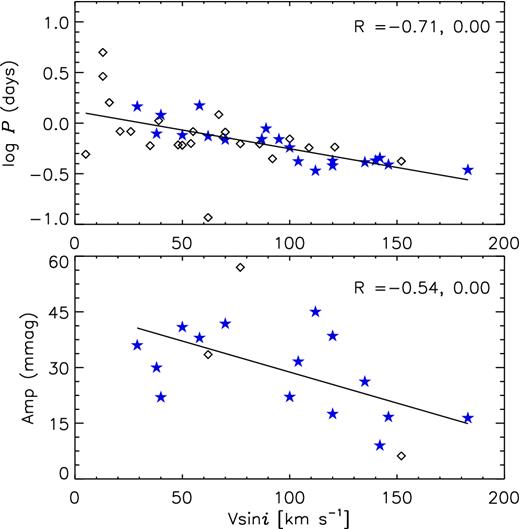
The comparison of vsin i with the pulsation period and amplitude of γ Dor stars. Bona-fide and candidate γ Dor variables are represented by stars and diamonds, respectively. The first number of R constant shows strength of the correlation (in the ideal case close to 1) while the second number represents deviations of points from the correlations (in the ideal case close to 0).
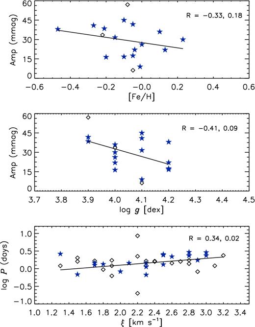
The relations between the pulsation period and pulsation amplitude of γ Dor stars and certain parameters given in x-axis. Stars and diamonds represent bona-fide and candidate γ Dor variables, respectively. The R constant has the same meaning as in Fig. 11.
The comprehensive abundance analysis of both bona-fide and candidate γ Dor stars was performed using the spectrum synthesis method. We compared chemical abundances of bona-fide γ Dor stars with those obtained for candidates and F type non-pulsating stars. According to these comparisons, no obvious differences were obtained. These stars have abundances close to the solar values (Asplund et al. 2009). The derived average iron abundances are equal 7.42 and 7.38 dex for bona-fide and candidate γ Dor stars, respectively. These values are also close to the solar iron abundances (7.50 dex).
In Fig. 13, the positions of the studied stars in the theoretical instability strips of γ Dor and δ Sct stars are given. The evolutionary tracks shown in this figure were calculated with the mesa (Modules for Experiments in Stellar Astrophysics) evolution code (Paxton et al. 2011, 2013, 2015). All the computed models have an initial hydrogen abundance of X = 0.7, the initial helium abundance of Y = 0.28 and use the AGSS09 metal mixture (Asplund et al. 2009). The initial metal abundance is Z = 0.02. The opal (Iglesias & Rogers 1996) opacity tables were used. All effects of rotation were neglected. The convective zones were determined by the Ledoux criterion. For the envelope, we adopted the parameter of the mixing length theory of αmlt = 2.0, as the theoretical instability strip of γ Dor stars were calculated with this value by Dupret et al. (2005).
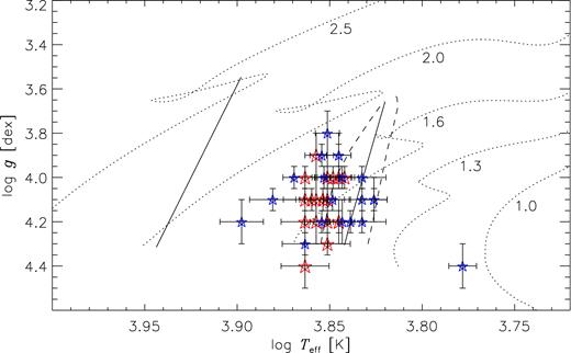
Positions of the bona-fide (bigger red stars) and candidate (small blue stars) γ Dor stars in the theoretical instability strips of the γ Dor (dashed-lines) and δ Sct (solid lines) stars (Dupret et al. 2005).
The positions of γ Dor stars in both theoretical instability strips have been discussed in the literature. In Uytterhoeven et al. (2011a), γ Dor stars were mostly found outside their theoretical instability strip. The same result was also presented in Grigahcène et al. (2010) and Tkachenko et al. (2012, 2013a), whereas Tkachenko et al. (2013b) found them inside the γ Dor instability strip within errors. As can be seen in Fig. 13, bona-fide γ Dor stars mostly cluster at the blue edge of the γ Dor instability strip, while some of them are located in δ Sct domain. Only HD 104860 is located outside those instability strips. Considering the received atmospheric parameters of this star, we conclude that HD 104860 is not a γ Dor variable.
In this study, we obtained accurate atmospheric parameters and chemical composition of a large sample of the γ Dor stars. They are essential in modelling of the pulsation and in the understanding of the real evolutionary status and stellar structure. As a result, we found that our stars are mostly located close to the blue edge of the γ Dor instability strip, where δ Sct pulsation (i.e. pressure modes) is also possible. This seems reduce a little the range of the γ Dor pulsation in the classical instability strip described by Uytterhoeven et al. (2011a). In the follow-up paper, we plan to perform a detailed spectroscopic study of SB2 γ Dor stars. The investigation of the sample of SB2 stars will give us the possibility to examine the probable differences of chemical abundances and atmospheric parameters with respect to the single stars studied in this paper.
The authors would like to thank the reviewer for useful comments and suggestions that helped to improve the publication. This work has been partly supported by the Scientific and Technological Research Council of Turkey (TUBITAK) grant numbers 2214-A and 2211-C. This article is a part of the PhD thesis of FKA. FKA wishes to express gratitude to professor Dr J. A. Guzik for all assistance given at the start of this project. EN acknowledges support from the NCN grant no. 2014/13/B/ST9/00902. The calculations have been carried out in Wrocław Centre for Networking and Supercomputing (http://www.wcss.pl), grant no. 214. We thank professor Dr R. O. Gray and Dr B. Smalley for their helpful comments. We are grateful to Dr D. Shulyak for putting the code for calculating SEDs at our disposal. We thank to Dr G. Catanzaro for putting the code for Balmer lines analysis at our disposal. ‘Ministerio de Economía y Competitividad’ (MINECO) and FEDER funds under the ‘Ramón y Cajal’ sub program, also acknowledges support by the European project SpaceInn (ref. 312844) within the European SPACE program FP7-SPACE-2011-1, and from Junta de Andalucía (Spanish) local government under project Contribuciãn Andaluza al proyecto espacial CoRoTs with reference P12-TIC-2469. This work is partially based on observations collected at La Silla Observatory, ESO (Chile) with the FEROS and HARPS spectrographs under programmes LP178.D-0361, LP182.D-0356, and LP185.D-0056. EP and MR acknowledge financial support from the FP7 project SpaceInn: Exploitation of Space Data for Innovative Helio and Asteroseismology and from PRIN-INAF 2014 Galactic Archaelogy. This research has made use of the SIMBAD data base, operated at CDS, Strasbourg, France.
REFERENCES
SUPPORTING INFORMATION
Additional Supporting Information may be found in the online version of this article:
Table 5. The average abundances and standard deviations of individual elements of stars.
Please note: Oxford University Press is not responsible for the content or functionality of any supporting materials supplied by the authors. Any queries (other than missing material) should be directed to the corresponding author for this article.
