Principal velocity surfaces in stellar dynamics

Lynden-Bell, D.

doi:10.1093/mnras/stw229

Abstract

Recent work by An and Evans has revived interest in the coordinate surfaces that lie along the principal axes of the stress tensor. Here we complete our list of non-axially symmetric systems with local integrals and prove that those principal velocity surfaces exist for all systems with three local integrals. We then demonstrate how systems in non-separable potentials evade the Eddington–An theorem by having distribution functions that lack perfect reflection symmetry in a meridional velocity component, and discuss other consequences of this remarkable theorem.

globular clusters: general, galaxies: kinematics and dynamics

1 INTRODUCTION

This paper was stimulated by the papers of An & Evans (2016) and Evans et al. (2016) that showed an intimate relationship between steady-state stellar systems with triaxial stress tensors aligned with any triply orthogonal coordinate system (the principal velocity surfaces) and the separability of motion in the potential in those coordinates. A relationship of this kind was first found in a great paper by Eddington (1915). His theorem states that if the distribution function is an anisotropic Maxwellian (i.e. a Schwarzschild 1907 distribution) at every point and if the three different principal axes of the resulting stress tensor lie perpendicular to a set of surfaces, then those surfaces must be confocal quadrics. Furthermore, the potential must be of the form that allows the equations of motion to separate in those ellipsoidal coordinates or in degenerate forms thereof.

Later workers including Chandrasekhar (1960) generalized the Schwarzschild distribution to include a mean motion. Thus the ellipsoidal hypothesis is that the distribution function is some function of |${({\boldsymbol v}-\overline{\boldsymbol v})\cdot{\cal {\boldsymbol A}}\cdot({\boldsymbol v}-\overline{\boldsymbol v})}+B$| where |${\cal {\boldsymbol A}}({\boldsymbol r})$| is a positive definite matrix, |${\overline{\boldsymbol v}({\boldsymbol r}})$| is the mean velocity and |$B({\boldsymbol r})$| is a scalar function of position |${\boldsymbol r}$|⁠.

Chandrasekhar (1960) virulently criticized Eddington for his unstated assumption that principal velocity surfaces existed at all. After referencing Eddington's work he writes ‘But unfortunately Eddington's treatment was based on a fundamental fallacy’, viz. the existence of principal velocity surfaces. As a counter example Chandrasekhar gave a system with helical symmetry but such a system is infinite and unrealistic. In fact, all axially symmetrical stellar systems inevitably have principal velocity surfaces and outside axial symmetry no known finite steady stellar system lacks them! Furthermore, despite his exhausting analysis Chandrasekhar (1939) appears to have missed the important separable systems found by Eddington [and now mistakenly called after Stackel (1893) who never derived them or their potentials]. I shall call these systems Eddingtonian. I have looked for these separable potentials in Chandrasekhar's voluminous paper but failed to find them although he quotes Eddington's later collaborator G.L.Clark and claims to be giving a more general treatment. In his paper Clark (1937) gives the integrals in the Eddingtonian systems. The part of my thesis (Lynden-Bell 1960) on time-dependent accretion discs was later written into a paper with Pringle (Lynden-Bell & Pringle 1974), but the major part was a redevelopment of stellar dynamics based on Jeans's theorem and integrals of motion without appeal to the restrictive ellipsoidal hypothesis.

However, I did appeal to some functional freedom in the potential within which the stars moved (Lynden-Bell 1962, hereafter Paper I). This paper correctly derived all the local integrals of axially symmetrical systems including the separable Eddingtonian systems in spheroidal coordinates. For systems lacking that symmetry it included a proof of the existence of principal velocity surfaces. However some years later, I think it was Stodolkiewicz of the Copernicus Astronomical Institute in Cracow who wrote pointing out that although my tables of local integrals gave |${\textstyle {\frac{1}{2} }\!}({{\boldsymbol r}\times {\boldsymbol v}})^2-\zeta (\theta )$| as an integral in the axially symmetrical potentials ψ = η(r) + ζ(θ)/r², they omitted the more general |${\textstyle {\frac{1}{2} }\!}({{\boldsymbol r}\times {\boldsymbol v}})^2-\zeta (\theta ,\phi )$| in the potentials ψ = η(r) + ζ(θ, ϕ)/r² that lack axial symmetry. My method ought to have found this more general case when I treated potentials out of axial symmetry. Here I find and correct the mistake that led to that omission, but, as it occurs prior to my proof of the existence of the principal velocity surfaces and the two are not unconnected, it is appropriate to revisit that also. The correction gives no extra systems other than that pointed out by Stodolkiewicz.

Appendix C of Evans et al. (2016), which is basically due to An, shows that Eddington's theorem can be proved without assuming either the ellipsoidal hypothesis or local integrals, but it requires both the existence of principal velocity surfaces and distribution functions with symmetries under the reversal of velocity components. This extended Eddington–An theorem, which is also proved in An & Evans (2016), re-emphasizes the importance of principal velocity surfaces and has remarkable consequences, but we show that it does NOT imply that all steady-state stellar systems which have stress tensors with unequal axes must have separable potentials. We also discuss some interesting unanswered questions raised by this theorem. Those less interested in local integrals or special potentials may find it useful to skip to Section 4 which concerns the application of the Eddington–An theorem to general axially symmetrical steady-state stellar systems.

2 LOCAL INTEGRALS REVISITED

My old analysis depends on the existence of local integrals, so a definition of them is needed. A stellar system that is steady as seen in fixed axes has a potential ψ = ζ(x, y, z) that is independent of time. All stars moving in this potential have their energies |$\varepsilon ={\textstyle {\frac{1}{2} }\!}{\boldsymbol v}^2-\zeta$| as integrals, i.e. constants of the motion. Likewise in potentials of the form ψ = η(r) + ζ(θ)/r² have not only ε but also L_z = Rv_ϕ and |$I={\textstyle {\frac{1}{2} }\!}({{\boldsymbol r}\times {\boldsymbol v}})^2-\zeta (\theta )$| as constants of motion. Here, R² = x² + y². It is seen that these integrals of the motion exist for a whole class of potentials which have functional freedoms. For the energy integral we have a three-dimensional functional freedom in our choice of ζ(x, y, z). For the angular momentum about the z-axis, L_z, we have a two-dimensional functional freedom in the potential ψ = ζ(r, θ). For the integral |${\textstyle {\frac{1}{2} }\!}{({\boldsymbol r}\times {\boldsymbol v})}^2-\zeta (\theta )$| we have two one-dimensional functional freedoms ζ(θ) and η(r). A local integral is a constant of the motion for a set of Hamiltonians |$H[{\boldsymbol p,r},\zeta (\lambda )]$| which we take to be |${\textstyle {\frac{1}{2} }\!}{\boldsymbol p}^2-\psi [{\boldsymbol r},\zeta (\lambda )]$|⁠. Here, ψ is some fixed function of its arguments and ζ is a freely variable function of its argument λ, which is a fixed function of position. The problem of finding local integrals is to determine what forms of the potential ψ and what forms of λ(x, y, z) allow integrals |$I({\boldsymbol p,r},\zeta )$| for any ζ(λ). These integrals are called local since they depend only on ζ at the point currently occupied, whereas they might have depended on ζ elsewhere, i.e. on a functional of ζ(λ).

2.1 Potentials of the form |$\psi [{\boldsymbol r},\zeta (\lambda ,\mu )]$|

First we consider potentials of the above form depending on an arbitrary function of two variables λ and μ which are assumed independent but need not have orthogonal surfaces. For |$I[{\boldsymbol p,r},\zeta (\lambda \cdot\mu )]$| to be a conserved integral we need the Poisson bracket [H, I] = 0 and hence

\begin{equation} {\boldsymbol p} \left[\frac{\mathrm{\partial} I}{\mathrm{\partial} {\boldsymbol r}}\big|_{\zeta }+\frac{\mathrm{\partial} I}{\mathrm{\partial} \zeta } \nabla \zeta \right]+\left[\frac{\mathrm{\partial} \psi }{\mathrm{\partial} {\boldsymbol r}}\big|_\zeta +\frac{\mathrm{\partial} \psi }{\mathrm{\partial} \zeta }\nabla \zeta \right]\cdot\frac{\mathrm{\partial} I}{{\mathrm{\partial} \boldsymbol p}}=0. \end{equation}

(1)

This must hold for all ζ(λ, μ) so

\begin{equation} \left[\frac{\mathrm{\partial} H}{\mathrm{\partial} {\boldsymbol p}}\frac{\mathrm{\partial} I}{\mathrm{\partial} \zeta }-\frac{\mathrm{\partial} H}{\mathrm{\partial} \zeta }\frac{\mathrm{\partial} I}{\mathrm{\partial} {\boldsymbol p}}\right]\cdot\nabla \zeta =0. \end{equation}

(2)

If I is of the form |$I(H,{{\boldsymbol p}\cdot{\boldsymbol n},{\boldsymbol r}}),$| this equation becomes

\begin{eqnarray*} -\frac{\mathrm{\partial} H}{\mathrm{\partial} \zeta }\frac{\mathrm{\partial} I}{\mathrm{\partial} {({\boldsymbol p}\cdot{\boldsymbol n})}}{{\boldsymbol n}\cdot\nabla }\zeta =0,\nonumber\end{eqnarray*}

which is clearly satisfied when |${\boldsymbol n}$| is any vector parallel to ∇λ × ∇μ. For a proof that this is the general solution, see Paper I. With I of this form [H, I] = 0 gives

\begin{equation} {\boldsymbol p}\cdot\left[\frac{\mathrm{\partial} I}{\mathrm{\partial} {\boldsymbol r}}\big|_{H,{{p}\cdot{n}}}+\frac{\mathrm{\partial} I}{\mathrm{\partial} ({{\boldsymbol p}\cdot{\boldsymbol n}})}\nabla {({\boldsymbol p}\cdot{\boldsymbol n})} \right]+\frac{\mathrm{\partial} I}{\mathrm{\partial} {({\boldsymbol p}\cdot{\boldsymbol n})}}{{\boldsymbol n}\cdot\nabla }\psi =0, \end{equation}

(3)

where |$\nabla \psi =\mathrm{\partial} \psi /\mathrm{\partial} {\boldsymbol r}|_\zeta +\mathrm{\partial} \psi /\mathrm{\partial} \zeta \nabla \zeta$|⁠. We now define

\begin{equation} {\boldsymbol K}=\left[\frac{\mathrm{\partial} I}{\mathrm{\partial} {\boldsymbol r}}\big|_{H,{{\boldsymbol p}\cdot{\boldsymbol n}}}\right]\big/\left[\frac{\mathrm{\partial} I}{\mathrm{\partial} {({\boldsymbol p}\cdot{\boldsymbol n})}}\big|_{H,{\boldsymbol r}}\right] \end{equation}

(4)

so equation (3) reads

\begin{equation} {{\boldsymbol p}\cdot{\boldsymbol K}+{\boldsymbol p}\cdot({\boldsymbol p}\cdot\nabla ){\boldsymbol n}+{\boldsymbol n}\cdot\nabla }\psi =0. \end{equation}

(5)

This must hold for all |${\boldsymbol p}$| and from its definition |${\boldsymbol K}$| is a function of |$H,{{\boldsymbol p}\cdot{\boldsymbol n},{\boldsymbol r}}$|⁠. In Paper I I saw that |${{\boldsymbol p}\cdot{\boldsymbol K}}$| had to be quadratic in |${\boldsymbol p}$| and wrongly deduced that |${\boldsymbol K}$| should be linear in |${\boldsymbol p}$|⁠. The term independent of |${\boldsymbol p}$| was also accommodated if |${\boldsymbol K}$| took the form |${{\boldsymbol K}= ({\boldsymbol p}\cdot{\boldsymbol n}){\boldsymbol G}({\boldsymbol r})-{\boldsymbol n}({\boldsymbol p}\cdot{\boldsymbol n})^{-1}({n}\cdot\nabla )}\psi$|⁠. What I failed to notice was that the more general form

\begin{equation} {{\boldsymbol K}=({\boldsymbol p}\cdot{\boldsymbol n}){\boldsymbol G}({\boldsymbol r})+{\boldsymbol n}({\boldsymbol p}\cdot{\boldsymbol n})}^{-1}[\alpha ({\boldsymbol r})H+\beta ({\boldsymbol r})] \end{equation}

(6)

would also give |${{\boldsymbol p}\cdot {\boldsymbol K}}$| quadratic in |${\boldsymbol p}$| and the |${\boldsymbol p}$|-independent term would be accounted for provided

\begin{equation} \alpha \psi -\beta ={{\boldsymbol n}\cdot\nabla }\psi . \end{equation}

(7)

It is this more general situation that we now explore. [The addition of a term in |${ ({{\boldsymbol p}\cdot{\boldsymbol n}})}^2$| inside the square bracket of equation (6) is merely equivalent to a change in |${\boldsymbol G}$| so is omitted without loss of generality.]

At constant H and |${{\boldsymbol p}\cdot{\boldsymbol n}}, \mathrm{\partial} I/\mathrm{\partial} {\boldsymbol r}$| is a pure gradient so from its definition |${\boldsymbol K}$| is parallel to a pure gradient and therefore with those quantities held fixed |${{\boldsymbol K}\cdot curl {\boldsymbol K}=0}$|⁠. This holds for all |${{\boldsymbol p}\cdot{\boldsymbol n}}$| so we deduce from (6) that

\begin{equation} {{\boldsymbol G}\cdot curl {\boldsymbol G}=0}, \end{equation}

(8)

and provided that not both α and β are zero

\begin{equation} {{\boldsymbol n}\cdot curl {\boldsymbol n}=0}. \end{equation}

(9)

So far |${\boldsymbol n}$| is any vector field parallel to ∇λ × ∇μ. We now study how our equations respond if we choose instead of |${\boldsymbol n}$| a different |${{\boldsymbol n}^{\ast }}=\kappa ({\boldsymbol r){\boldsymbol n}}$|⁠, where κ is any scalar function of position. We write

\begin{eqnarray*} I[H,{{\boldsymbol p}\cdot{\boldsymbol n},{\boldsymbol r}}]=I^{\ast }[H,{{\boldsymbol p}\cdot{\boldsymbol n}^{\ast },{\boldsymbol r}}]=I^{\ast }[H,\kappa {{\boldsymbol p}\cdot{\boldsymbol n},{\boldsymbol r}}] \nonumber\end{eqnarray*}

then

\begin{eqnarray*} \mathrm{\partial} I/\mathrm{\partial} {\boldsymbol r}|_{H,{{p}\cdot{n}}}= \mathrm{\partial} I^{\ast }/\mathrm{\partial} {\boldsymbol r}|_{H,{{p}\cdot{n}}^{\ast }}+ [\mathrm{\partial} I^{\ast }/\mathrm{\partial} {{\boldsymbol p}\cdot{\boldsymbol n}^{\ast }}]{{\boldsymbol p}\cdot{\boldsymbol n}}\nabla \kappa \nonumber\end{eqnarray*}

and

\begin{eqnarray*} \mathrm{\partial} I/\mathrm{\partial} {{\boldsymbol p}\cdot{\boldsymbol n}}|_{H,{\boldsymbol r}}= \kappa \mathrm{\partial} I^{\ast }/\mathrm{\partial} {{\boldsymbol p}\cdot{\boldsymbol n}^{\ast }}|_{H,{\boldsymbol r}}\nonumber\end{eqnarray*}

so

\begin{eqnarray*} \frac{\mathrm{\partial} I/\mathrm{\partial} {\boldsymbol r}}{\mathrm{\partial} I/\mathrm{\partial} {{\boldsymbol p}\cdot{\boldsymbol n}}}={\boldsymbol K}=\frac{\mathrm{\partial} I^{\ast }/{\mathrm{\partial} \boldsymbol r}}{\kappa \mathrm{\partial} I^{\ast }/\mathrm{\partial} {{\boldsymbol p}\cdot{\boldsymbol n}}^{\ast }}+{{\boldsymbol p}\cdot{\boldsymbol n}}\nabla \ln \kappa ,\nonumber\end{eqnarray*}

hence writing

\begin{eqnarray*} \frac{\mathrm{\partial} I^{\ast }/{\mathrm{\partial} \boldsymbol r}}{\mathrm{\partial} I^{\ast }/\mathrm{\partial} {{\boldsymbol p}\cdot{\boldsymbol n}}^{\ast }}={{\boldsymbol K}^{\ast }=({\boldsymbol p}\cdot{\boldsymbol n}^{\ast }){\boldsymbol G}^{\ast }+\frac{{\boldsymbol n}^{\ast }}{({\boldsymbol p}\cdot{\boldsymbol n}^{\ast })}}(\alpha ^{\ast }H+\beta ^{\ast }),\nonumber\end{eqnarray*}

by comparing multiples of |${{\boldsymbol p}\cdot{\boldsymbol n}}$| and then |${\boldsymbol n}$| we see

\begin{eqnarray*} {{\boldsymbol p}\cdot{\boldsymbol n}} ({{\boldsymbol G}} - \nabla \ \text{ln}\ \kappa ) &=& ({{\boldsymbol p}\cdot{\boldsymbol n}}){{\boldsymbol G}^{\ast }},\\ \frac{{\boldsymbol n}}{({{\boldsymbol p}\cdot{\boldsymbol n}})} (\alpha H + \beta )&=& \frac{{\boldsymbol n}}{{{\boldsymbol p}\cdot{\boldsymbol n}}}\left(\frac{H\alpha ^{\ast }}{\kappa }+\frac{\beta ^{\ast }}{\kappa }\right). \end{eqnarray*}

As this holds for all |${{\boldsymbol p}\cdot{\boldsymbol n}}$| and all H we deduce that

\begin{equation} {{\boldsymbol G}^{\ast }={\boldsymbol G}-\nabla }\ln \kappa ;\qquad \alpha ^{\ast }=\kappa \alpha ,\qquad \beta ^{\ast }=\kappa \beta . \end{equation}

(10)

Now like the previous argument for |${\boldsymbol G}$| we have |${{\boldsymbol G}^{\ast }\cdot curl {\boldsymbol G}^{\ast }=0}$|⁠, hence

\begin{equation} -(\nabla \ln \kappa )\cdot {curl {\boldsymbol G}}=0, \end{equation}

(11)

but this must hold whatever we choose for κ so |${curl {\boldsymbol G}=0}$|⁠, which implies that |${\boldsymbol G}$| can be written as

\begin{equation} {\boldsymbol G}=\nabla \ln \gamma . \end{equation}

(12)

Using this result in equation (10) and choosing κ = γ we see that we can make |${{\boldsymbol G}^{\ast }}=0$| and then

\begin{equation} {{\boldsymbol K}^{\ast }=\frac{ n^{\ast }}{p\cdot n^{\ast }}} (\alpha ^{\ast }H+\beta ^{\ast }). \end{equation}

(13)

From the starred version of equation (5) we have, using the summation convention over repeated indices

\begin{equation} \alpha ^{\ast }H+\beta ^{\ast }+p_ip_j\mathrm{\partial} _i n^{\ast }_j+n^{\ast }_i\mathrm{\partial} _i\psi =0. \end{equation}

(14)

Since p_i is arbitrary the quadratic terms in it must vanish separately so

\begin{equation} \mathrm{\partial} _i n^{\ast }_j+\mathrm{\partial} _j n^{\ast }_i=-\alpha ^{\ast }\delta _{ij}, \end{equation}

(15)

while the terms independent of p_i give the starred version of equation (7).

\begin{equation} \alpha ^{\ast }\psi -\beta ^{\ast }={{\boldsymbol n}^{\ast }\cdot\nabla }\psi . \end{equation}

(16)

Our problem now splits into three separate cases. (i) α* ≠ 0, (ii) α* = 0, β* ≠ 0, (iii) α* = β* = 0. In cases (i) and (ii) we have from the starred version of equation (9) |${{\boldsymbol n}^{\ast }\cdot curl {\boldsymbol n}^{\ast }=0}$|⁠, which implies that |${{\boldsymbol n}^{\ast }}=N\nabla \nu$|⁠, where N is a scalar function of position. Since at constant |${{{\boldsymbol p}\cdot{\boldsymbol n}}^{\ast },\ {\boldsymbol K}^{\ast }}$| is parallel to the gradient of ν, it follows that the coefficients must be functions of ν. Thus |$I=I(H, {{{\boldsymbol p}\cdot{\boldsymbol n}}^{\ast }},\nu )$|⁠, and both Nα* and Nβ* and therefore β*/α* are all functions of ν. In considering the implications of equation (15) it is useful to think of |${{\boldsymbol n}^{\ast }}$| as a displacement vector in space. Then |${\textstyle {\frac{1}{2} }\!}(\mathrm{\partial} _i n^{\ast }_j+\mathrm{\partial} _j n^{\ast }_i)$| is the strain tensor due to such a displacement. If the strain were zero then the solution would be a rigid body displacement. However we see from (15) that in case (i) it is not zero but rather an isotropic expansion or contraction at each point. Such a displacement preserves angles and its divergence gives the volume expansion factor of the conformal transformation at each point of space. We show in the Appendix that the only three-dimensional conformal transformations in a flat space are uniform expansions or contractions with α* constant, or inversions with α* = k/r². However we already know that Nα* is a function of ν, so |${{\boldsymbol n}^{\ast }}=(1/\alpha ^{\ast })\nabla \tilde{\nu }$| where |$\tilde{\nu }$| is a function of ν. So returning to equation (15) in dyadic notation we now have with δ the unit tensor

\begin{equation} \nabla [(1/\alpha ^{\ast })\nabla \tilde{\nu }|_S=-{\textstyle {\frac{1}{2} }\!}\alpha ^{\ast } \delta , \end{equation}

(17)

where the suffix S denotes that the tensor is symmetrized. We treat below the situation with α* constant and show in the Appendix that there are no solutions when α* = k/r². Solving the 1,2 component we find |$\tilde{\nu }=u_I(x_2,x_3)+u_{II}(x_1,x_3)$| but applying the 2,3 and 3,1 components this solution reduces to |$\tilde{\nu }=u_1(x_1)+u_2(x_2)+u_3(x_3)$|⁠. Finally applying the 1,1 2,2 and 3,3 components we find

\begin{eqnarray*} u_1^{\prime \prime }=u_2^{\prime \prime }=u_3^{\prime \prime }=-{\textstyle {\frac{1}{2} }\!}\alpha ^{{\ast }2} \nonumber\end{eqnarray*}

so

\begin{eqnarray*} u_1=-\textstyle {\frac{1}{4}\!} \alpha ^{{\ast }2}x_1^2+c_1 x_1+d_1\cdot\nonumber\end{eqnarray*}

Since α*² ≠ 0, we may take a new origin to remove the linear terms and we then find |${\boldsymbol n}^{\ast }=(1/\alpha ^{\ast })\nabla \tilde{\nu }=-{\textstyle {\frac{1}{2} }\!}\alpha ^{\ast }{\boldsymbol r}$|⁠. This implies that |$\tilde{\nu },\nu$| are functions of the scalar r. We now insert this result into equation (16) to find the form of potential involved, remembering that β*/α* must now be a function of r too. Dividing by α* we find |$\psi =\beta ^{\ast }/\alpha ^{\ast }-{\textstyle {\frac{1}{2} }}r\mathrm{\partial} \psi /\mathrm{\partial} r$|⁠, hence

\begin{eqnarray} &&{\mathrm{\partial} (r^2\psi )/\mathrm{\partial} r = 2r\beta ^{\ast }/\alpha ^{\ast },}\nonumber \\ &&{\psi =\eta (r)+\zeta (\theta ,\phi )/r^2, } \end{eqnarray}

(18)

where η is r⁻² times the integral of 2rβ*/α* which is a function of r. Thus we have recovered the potential that was missing from my table in Paper I.

The constant of the motion is most readily derived directly; writing |${\hat{\boldsymbol r}={\boldsymbol r}}/r$|

\begin{eqnarray} &&{\frac{{\rm d}{\boldsymbol v}}{{\rm d}t}=\nabla \psi =\left(\eta ^{\prime }-2\frac{\zeta }{r^3}\right){\hat{\boldsymbol r}}+\frac{1}{r^2}\nabla \zeta}\nonumber\\ &&{ {\rm d/d}t({\boldsymbol r}\times {\boldsymbol v}) {\rm d}t=r^{-2}{{\boldsymbol r}\times \nabla }\zeta} \nonumber \\ &&{\frac{{\rm d}({{\boldsymbol r}\times {\boldsymbol v}})^2}{{\rm d}t}=({\hat{\boldsymbol r}\times {\boldsymbol v}})\cdot({\hat{\boldsymbol r}\times \nabla }\zeta )=({{\boldsymbol v}-{\boldsymbol v}\cdot\hat{{\boldsymbol r}}\hat{{\boldsymbol r}}})\cdot\nabla \zeta }\nonumber\\ &&{\qquad\qquad\;\,={\boldsymbol v}\cdot\nabla \zeta ={\rm d}\zeta /{\rm d}t} \end{eqnarray}

(19)

which demonstrates that |${\textstyle {\frac{1}{2} }\!}{({\boldsymbol r}\times {\boldsymbol v}})^2-\zeta (\theta ,\phi )$| is a constant of the motion and completes case (i).

In case (ii) α* = 0 so equation (15) shows that |${{\boldsymbol n}^{\ast }}$| is a rigid displacement, however it has orthogonal surfaces since β* is not zero. The only rigid displacements with orthogonal surfaces are rigid rotation and pure displacements, so by suitably orienting our axes we may take either |${{\boldsymbol n}^{\ast }}=\Omega R \hat{{\bf \phi }}=\Omega R^2\nabla \phi$|⁠, case (iia), or along |${\hat{\boldsymbol z}}=\nabla z$|⁠, case (iib).

In case (iia) N = ΩR² equation (16) gives β* = −Ω∂ψ/∂ϕ, but Nβ* = ΩR²β* is a function of |$\tilde{\nu }$|⁠, which is now ϕ. Thus ∂ψ/∂ϕ = η′(ϕ/R²), say, so ψ = ζ(R, z) + η(ϕ) and the integral is easily found to be |${\textstyle {\frac{1}{2} }\!}(Rv_\phi )^2-\eta (\phi )$|⁠. Case (iib) is trivial ψ = ζ(x, y) + η(z) with the integral |${\textstyle {\frac{1}{2} }\!}v_z^2-\eta (z)$|⁠.

Finally, we come to case (iii). Here |${{\boldsymbol n}^{\ast }}$| is a rigid displacement and |${{\boldsymbol n}^{\ast }}\cdot\nabla \psi =0$| so the potential is unchanged along the displacement. Without loss of generality the displacement can be taken to be a displacement along the z-axis accompanied by a rotation about that axis so the lines of the displacement are helical. The potential is of the form ψ = ζ(x′, y′) where x′ = xcos (z/l) + ysin (z/l); y′ = −xsin (z/l) + ycos (z/l) where l is the height at which the helix has turned by one radian. By symmetry the conserved integral is a combination of the linear and angular momentum about the axis I = v_z + L_z/l = v_z + (xv_y − yv_x)/l. Instead of this symmetry argument we may calculate

\begin{eqnarray*} &&{\frac{{\rm d}v_z}{{\rm d}t}=\frac{\mathrm{\partial} \zeta }{\mathrm{\partial} z}=\frac{\mathrm{\partial} \zeta }{\mathrm{\partial} x^{\prime }} [-x\sin (z/l)+y\cos (z/l)]/l}\nonumber \\ &&{\qquad\qquad\qquad-\frac{\mathrm{\partial} \zeta }{\mathrm{\partial} y^{\prime }}[x\cos (z/l)+y\sin (z/l)]/l}\nonumber \\ &&{\frac{{\rm d}v_y}{{\rm d}t}=\frac{\mathrm{\partial} \zeta }{\mathrm{\partial} y }=\frac{\mathrm{\partial} \zeta }{\mathrm{\partial} x^{\prime }}[\sin (z/l]+\frac{\mathrm{\partial} \zeta }{\mathrm{\partial} y^{\prime }}[\cos (z/l)]}\nonumber \\ &&{\frac{{\rm d}v_x}{{\rm d}t}=\frac{\mathrm{\partial} \zeta }{\mathrm{\partial} x} =\frac{\mathrm{\partial} \zeta }{\mathrm{\partial} x^{\prime }}[\cos (z/l]-\frac{\mathrm{\partial} \zeta }{\mathrm{\partial} y^{\prime }}[\sin (z/l)]} \end{eqnarray*}

thus

\begin{equation} {\rm d/d}t[v_z+(x v_y-y v_x)/l]=0. \end{equation}

(20)

This is Chandrasekhar's infinite helical system on which he based his rejection of Eddington's paper.

2.2 Potentials of the form |$\psi [{\boldsymbol r},\zeta (\lambda ),\eta (\mu )]$|

In determining all the axially symmetrical local integrals in Paper I we sought integrals in potentials with one free function of one variable but those found had two free functions. Except for those potentials allowing an integral linear in the velocities, we see this again in Table 1 in that the free functions η arose in the solutions without being requested. To gain a powerful handle on systems without axial symmetry we now seek integrals in potentials which have two free functions ζ(λ), η(μ) of two independent variables λ, μ. We shall not require λ and μ to have orthogonal surfaces but shall show shortly that such an existence of the type of integral sought enforces that. We shall require that the potentials are not merely special cases of the systems given in Table 1 since the arbitrary functions, ζ, of two variables can be chosen as two functions each of a different single variable in many ways. Such systems would merely give us back special cases of the systems in Table 1. We now look for an integral |$I=I({{\boldsymbol p},{\boldsymbol r}},\zeta ,\eta )$| in all the potentials of the form |$\psi [{\boldsymbol r},\zeta (\lambda ),\eta (\mu )]$|⁠. The condition that the Poisson bracket [H, I] = 0 for all ζ and all η leads to, cf. equation (2),

\begin{equation} \left(\frac{\mathrm{\partial} H\ \mathrm{\partial} I}{\mathrm{\partial} {\boldsymbol p} \ \mathrm{\partial} \zeta }-\frac{\mathrm{\partial} H\ \mathrm{\partial} I}{\mathrm{\partial} \zeta \ \mathrm{\partial} {\boldsymbol p}}\right)\nabla \zeta +\left(\frac{\mathrm{\partial} H\ \mathrm{\partial} I}{\mathrm{\partial} {\boldsymbol p} \ \mathrm{\partial} \eta }-\frac{\mathrm{\partial} H\ \mathrm{\partial} I}{\mathrm{\partial} \eta \ \mathrm{\partial} {\boldsymbol p}}\right)\nabla \eta =0. \end{equation}

(21)

The two terms must vanish separately since λ and μ are independent. At any point let |$p_\Lambda$| be the component along ∇λ and p_n be the component along ∇λ × ∇μ and let p₂ be the component along an axis perpendicular to those. Then the vanishing of the first term above implies that I only involves ζ via H so it must be of the form I = I⁽¹⁾(H, p₂, p_n, η) while the vanishing of the second implies the form |$I=I^{(2)}(H,\ a p_2+b p_\Lambda ,\ p_n,{\boldsymbol r},\zeta )$| where |$a p_2+b p_\Lambda$| is the component perpendicular to ∇μ and a and b are direction cosines. Now in |$I^{(1)},\ p_\Lambda$| is only involved via its square through H, while in I⁽²⁾ it appears in linear combination with p₂. These can only be consistent if (1) b = 0 or (2) I⁽²⁾ is independent of its second argument or (3) a = 0 and I⁽²⁾ is only dependent on the square of that argument. Option (1) has ∇μ parallel to ∇λ, which is forbidden as they have to be independent. Option (2) leaves I of the form that we investigated in the last section and gives nothing new, so we are left with option (3) a = 0 which implies |$p_\Lambda$| and p_n are perpendicular to ∇μ and ∇μ.∇λ = 0. Thus we may call p₂, p_M, where this M is a capital Mu, and the surfaces of constant λ and constant μ are orthogonal. To get a triply orthogonal coordinate system we still have to prove that |${\boldsymbol n}$| is orthogonal to a set of surfaces. With minor redefinition we can now write |$I=I^{(1)}(H,p_M^2,p_n,{\boldsymbol r},\eta )=I^{(2)}(H,p_\Lambda ^2,p_n,{\boldsymbol r},\zeta )$|⁠. In |$I^{(1)}, p_\Lambda$| and ζ are only involved in the combination that is in |$H, {\textstyle {\frac{1}{2} }\!}p_\Lambda ^2-\psi [{\boldsymbol r},\zeta (\lambda ),\eta (\mu )]$|⁠. However I⁽²⁾ cannot be independent of its second argument for the reasons given above, so it involves |$p_\Lambda ^2,{\boldsymbol r}$| and ζ without η. This can only happen if some combination of |${\textstyle {\frac{1}{2} }\!}p_\Lambda ^2-\psi [{\boldsymbol r},\zeta (\lambda ),\eta (\mu )],{\boldsymbol r},\eta$| is independent of η for all |$p_\Lambda$|⁠. This only occurs if |$\psi ({\boldsymbol r},\zeta ,\eta )$| separates in the form |$\psi =\psi ^{(1)}({\boldsymbol r},\zeta )+\psi ^{(2)}({\boldsymbol r},\eta )$| for then

Table 1.

Open in new tab

Potentials with free ζ(λ, μ), η(ν) and their local integrals. R² = x² + y².

Potential ψ	Integrals
ζ(x, y, z)	\|$\varepsilon ={\textstyle {\frac{1}{2} }\!}{\boldsymbol v}^2-\zeta$\|
η(r) + ζ(θ, ϕ)/r²	\|$\varepsilon ,{\textstyle {\frac{1}{2} }\!}({{\boldsymbol r}\times v})^2-\zeta (\theta ,\phi )$\|
ζ(R, z) + η(ϕ)/R²	\|$\varepsilon ,{\textstyle {\frac{1}{2} }\!}R^2 v_\phi ^2-\eta (\phi )$\|
ζ(x, y) + η(z)	\|$\varepsilon ,{\textstyle {\frac{1}{2} }\!}v_z^2-\eta (z)$\|
ζ(R, z)	ε, Rv_ϕ
ζ(x, y)	ε, v_z
ζ(x′, y′)	ε, v_z + Rv_ϕ/l.

Potential ψ	Integrals
ζ(x, y, z)	\|$\varepsilon ={\textstyle {\frac{1}{2} }\!}{\boldsymbol v}^2-\zeta$\|
η(r) + ζ(θ, ϕ)/r²	\|$\varepsilon ,{\textstyle {\frac{1}{2} }\!}({{\boldsymbol r}\times v})^2-\zeta (\theta ,\phi )$\|
ζ(R, z) + η(ϕ)/R²	\|$\varepsilon ,{\textstyle {\frac{1}{2} }\!}R^2 v_\phi ^2-\eta (\phi )$\|
ζ(x, y) + η(z)	\|$\varepsilon ,{\textstyle {\frac{1}{2} }\!}v_z^2-\eta (z)$\|
ζ(R, z)	ε, Rv_ϕ
ζ(x, y)	ε, v_z
ζ(x′, y′)	ε, v_z + Rv_ϕ/l.

Table 1.

Open in new tab

Potentials with free ζ(λ, μ), η(ν) and their local integrals. R² = x² + y².

Potential ψ	Integrals
ζ(x, y, z)	\|$\varepsilon ={\textstyle {\frac{1}{2} }\!}{\boldsymbol v}^2-\zeta$\|
η(r) + ζ(θ, ϕ)/r²	\|$\varepsilon ,{\textstyle {\frac{1}{2} }\!}({{\boldsymbol r}\times v})^2-\zeta (\theta ,\phi )$\|
ζ(R, z) + η(ϕ)/R²	\|$\varepsilon ,{\textstyle {\frac{1}{2} }\!}R^2 v_\phi ^2-\eta (\phi )$\|
ζ(x, y) + η(z)	\|$\varepsilon ,{\textstyle {\frac{1}{2} }\!}v_z^2-\eta (z)$\|
ζ(R, z)	ε, Rv_ϕ
ζ(x, y)	ε, v_z
ζ(x′, y′)	ε, v_z + Rv_ϕ/l.

Potential ψ	Integrals
ζ(x, y, z)	\|$\varepsilon ={\textstyle {\frac{1}{2} }\!}{\boldsymbol v}^2-\zeta$\|
η(r) + ζ(θ, ϕ)/r²	\|$\varepsilon ,{\textstyle {\frac{1}{2} }\!}({{\boldsymbol r}\times v})^2-\zeta (\theta ,\phi )$\|
ζ(R, z) + η(ϕ)/R²	\|$\varepsilon ,{\textstyle {\frac{1}{2} }\!}R^2 v_\phi ^2-\eta (\phi )$\|
ζ(x, y) + η(z)	\|$\varepsilon ,{\textstyle {\frac{1}{2} }\!}v_z^2-\eta (z)$\|
ζ(R, z)	ε, Rv_ϕ
ζ(x, y)	ε, v_z
ζ(x′, y′)	ε, v_z + Rv_ϕ/l.

\begin{eqnarray*} {\textstyle {\frac{1}{2} }\!}p_\Lambda ^2-\psi [{\boldsymbol r},\zeta ,\eta ]-\psi ^{(2)}({\boldsymbol r},\eta )= {\textstyle {\frac{1}{2} }\!}p_\Lambda ^2-\psi ^{(1)}[{\boldsymbol r},\zeta )\cdot\nonumber\end{eqnarray*}

Thus we may express I in either of the forms

\begin{eqnarray*} I&=&I\left[H,{\textstyle {\frac{1}{2} }\!}p_\Lambda ^2-\psi ^{(1)}({\boldsymbol r},\zeta (\lambda )),p_n,{\boldsymbol r}\right]\nonumber \\ &=& J\left[H,{\textstyle {\frac{1}{2} }\!}p_M^2-\psi ^{(2)}({\boldsymbol r},\eta (\mu )),p_n,{\boldsymbol r}\right]. \end{eqnarray*}

3 The existence of Eddington's principal velocity surfaces

Henceforth we write |${\hat{\boldsymbol \lambda }},{\hat{\boldsymbol \mu }}$| for the unit vectors parallel to ∇λ and ∇μ, respectively, and we set |${\boldsymbol n}={\hat{\boldsymbol \lambda }}\times {\hat{\boldsymbol \mu }}$| so that it too is a unit vector. We write I in the form |$I(H,{\textstyle {\frac{1}{2} }\!}({\boldsymbol p}\cdot{\hat{\boldsymbol \lambda }})^2-\psi ^{(1)},{{\boldsymbol p}\cdot{\boldsymbol n}},{\boldsymbol r})$| and use a suffix 2 to denote its differentiation with respect to its second argument, etc. As in Paper I we pick out from [H, I] = 0 those terms that reverse sign when |$p_\Lambda \rightarrow -p_\Lambda$| and also reverse sign when p_M → −p_M. Since [H, I] = 0 for all |${\boldsymbol p}$| these terms are also zero. They give

\begin{eqnarray} &&{I_2 p_\Lambda p_M p_n({\boldsymbol n}\cdot({\hat{\boldsymbol \mu }}\cdot\nabla ){\hat{\boldsymbol \lambda }}+{\hat{\boldsymbol \mu }}\cdot({\boldsymbol n}\cdot\nabla ){\hat{\boldsymbol \lambda }})}\nonumber \\ &&{\quad+\; I_3 p_\Lambda p_M({\hat{\boldsymbol \mu }}\cdot({\hat{\boldsymbol \lambda }}\cdot\nabla {\boldsymbol n}+{\hat{\boldsymbol \lambda }}\cdot({\hat{\boldsymbol \mu }}\cdot\nabla ){\boldsymbol n}) =0 } \end{eqnarray}

(22)

This involves the symmetry exploited by An. We now show that the coefficient of I₃ is zero. Since |${\hat{\boldsymbol \lambda }}\cdot{\hat{\boldsymbol \mu }}=0$|⁠,

\begin{eqnarray*} 0=\nabla ({\hat{\boldsymbol \lambda }}\cdot{\hat{\boldsymbol \mu }})={\hat{\boldsymbol \lambda }}\times {curl}{\hat{\boldsymbol \mu }}+{\hat{\boldsymbol \mu }}\times {curl}{\hat{\boldsymbol \lambda }}+({\hat{\boldsymbol \lambda }}\cdot\nabla ){\hat{\boldsymbol \mu }}+({\hat{\boldsymbol \mu }}\cdot\nabla ){\hat{\boldsymbol \lambda }}\nonumber\end{eqnarray*}

Taking the dot product with |${\boldsymbol n}$| and exchanging the dot and the times in the first two terms they become |${\hat{\boldsymbol \mu }}\cdot {\bf curl} {\hat{\boldsymbol \mu }}$| and |$-{\hat{\boldsymbol \lambda }}\cdot{\bf curl} {\hat{\boldsymbol \lambda }}$| both of which are zero since |${\hat{\boldsymbol \lambda }},{\hat{\boldsymbol \mu }}$| have orthogonal surfaces. We are left with

\begin{equation} ({\hat{\boldsymbol \lambda }}\cdot\nabla ){\hat{\boldsymbol \mu }}+({\hat{\boldsymbol \mu }}\cdot\nabla ){\hat{\boldsymbol \lambda }}=0. \end{equation}

(23)

But since |${\hat{\boldsymbol \mu }}\cdot{\boldsymbol n}=0,$|

\begin{eqnarray*} 0=({\hat{\boldsymbol \lambda }}\cdot\nabla )({\hat{\boldsymbol \mu }}\cdot{\boldsymbol n})={\boldsymbol n}\cdot({\hat{\boldsymbol \lambda }}\cdot\nabla ){\hat{\boldsymbol \mu }}+{\hat{\boldsymbol \mu }}({\hat{\boldsymbol \lambda }}\cdot\nabla ){\boldsymbol n}\cdot\nonumber\end{eqnarray*}

Using this and the similar relationship with the roles of |${\hat{\boldsymbol \mu }}$| and |${\hat{\boldsymbol \lambda }}$| reversed, equation (23) becomes

\begin{eqnarray*} {\hat{\boldsymbol \mu }}\cdot({\hat{\boldsymbol \lambda }}\cdot\nabla ){\boldsymbol n}+{\hat{\boldsymbol \lambda }}\cdot({\hat{\boldsymbol \mu }}\cdot\nabla ){\boldsymbol n} =0\nonumber\end{eqnarray*}

so the coefficient of I₃ vanishes.

Following the argument on |$\nabla ({\hat{\boldsymbol \lambda }}\cdot{\hat{\boldsymbol \mu }})$| above we look at |$\nabla ({\hat{\boldsymbol \mu }}\cdot{\boldsymbol n})$| and find

\begin{eqnarray} 0=({\hat{\boldsymbol \lambda }}\cdot\nabla )({\hat{\boldsymbol \mu }}\cdot{\boldsymbol n})={{\boldsymbol n}\cdot curl\ {\boldsymbol n}}+0 \nonumber \\ \ \ \ \ +\,{\hat{\boldsymbol \lambda }}\cdot({\boldsymbol n}\cdot\nabla ){\hat{\boldsymbol \mu }}+{\hat{\boldsymbol \lambda }}\cdot({\hat{\boldsymbol \mu }}\cdot\nabla ){{\boldsymbol n}.} \end{eqnarray}

(24)

But

\begin{eqnarray*} {\hat{\boldsymbol \lambda }}\cdot({\boldsymbol n}\cdot\nabla ){\hat{\boldsymbol \mu }}+{\hat{\boldsymbol \lambda }}\cdot({\hat{\boldsymbol \mu }}\cdot\nabla ){\boldsymbol n}=-{\boldsymbol n}\cdot({\hat{\boldsymbol \mu }}\cdot\nabla ){\hat{\boldsymbol \lambda }}-{\hat{\boldsymbol \mu }}\cdot({\boldsymbol n}\cdot\nabla ){\hat{\boldsymbol \lambda }}\nonumber\end{eqnarray*}

which should be compared with the coefficient of I₂ in equation (22). So using equation (24) equation (22) becomes

\begin{equation} I_2 p_\Lambda p_M p_n({{\boldsymbol n}\cdot curl\ {\boldsymbol n}})=0. \end{equation}

(25)

Now I₂ = 0 only leads us back to our former discussion of integrals depending on a free function of two variables and special cases thereof. To get an integral not contained therein we need I₂ ≠ 0 in which case |${{\boldsymbol n}\cdot curl\ {\boldsymbol n}=0}$|⁠, so |${\boldsymbol n}$| has orthogonal surface and those together with λ, μ form a triply orthogonal coordinate system. It is then possible to introduce their canonical momenta rather than the momentum components |$p_\Lambda ,\ p_M,\ p_n$| used above. With such surfaces one may prove Eddington's theorem without the ellipsoidal hypothesis and find the separable potentials and the integrals as was done earlier in my thesis and as sketched in Paper I.

Beside G.L. Clark's work there are fine explorations of these systems particularly by Kuzmin (1952) which were later extended by Tim De Zeeuw (1985a,b). An axially symmetrical potential with three integrals that are not in involution, which was mentioned in Paper I as having a non-axially symmetrical integral, is discussed in Lynden-Bell & Booth (2009). Local integrals in systems with vector potentials are catalogued in Lynden-Bell (2000). Configuration invariants e.g. integrals that exist for one value of the energy only, are given for two-dimensional systems in Hall (1985) and were discussed earlier by Stodolkiewicz (1974). In axially symmetric potentials the effective potential contains |${\textstyle {\frac{1}{2} }\!} L_z^2/R^2$|⁠. Although this separates in the classical spheroidal coordinates it does not separate in the conformally related coordinates used by Hall, so his configuration invariants applied to three-dimensional but axially symmetric systems can only hold for one value of the angular momentum as well as one energy.

4 TOO TRUE TO BE GOOD

We return to the theorem of appendix C of Evans et al. This we apply to axially symmetrical steady-state stellar systems which have unequal principal stresses and inevitably have principal velocity surfaces. The stars can consist of tracers since no assumption of self-gravitation is involved. These tracers can be any steady-state subsystem e.g. stars defined by a definite metal abundance or even stars on a particular axially symmetric class of orbits. If the coordinates defining the principal velocity surfaces are called λ, μ, ϕ a relevant version of the theorem shows that provided the distribution function depends only on the square of p_λ rather than p_λ itself, then the potential in which those tracer stars move MUST be of the separable Eddingtonian form ψ = [ζ(λ) − η(μ)]/(λ − μ) and λ, μ must be spheroidal coordinates. This sounds too good to be true but it is really too true to be useful. Take a smooth axially symmetrical potential NOT of the special separable Eddingtonian form that gives a third local integral. Release into it a number of stars with low angular momenta given their positions of release. Let these stars have negligible total mass. Although such a system never reaches a steady state, nevertheless after a long time the system will ‘converge in the mean’ to one. Following the early work of Contopoulos (1960) and later work by Henon (1976) we now know that despite the non-separability of the motions nevertheless most stars will have effective third integrals which will preserve the strong radial motions that they have initially. Thus, as in systems constructed under Schwarzschild's precepts they will generate steady axially symmetric systems with tri-axial stress tensors. These will have principal velocity surfaces because of the axial symmetry. However the potential will not be of the separable Eddingtonian type since we specified the potential so. Although such systems may appear to contradict the theorem of appendix C in Evans et al. the devil lurks in the detail. The proof of the theorem requires symmetry of the distribution function under the operation v_λ → −v_λ. What is really proved is that such symmetries in the distribution function can only occur for the separable systems. The systems constructed in non-separable potentials will have effective third integrals but will lack the v_λ → −v_λ symmetry about the λ principal velocity surface. The theorem does not dictate the form of the potential but rather it tells us that this symmetry in the distribution function is a unique property of separable systems. While this is itself remarkable and interesting it does not tell us that all reasonable stellar systems should have separable potentials. However, the Eddington–An theorem raises questions about possible forms for the principal velocity surfaces. Can they be cylindrical everywhere as postulated by Cappellari (2008) without having the v_R ⇒ −v_R symmetry which implies that the potential is separable and of the unacceptable form ψ = ψ₁(R) + ψ₂(z). Indeed, if we postulate that the principal velocity surfaces are prolate spheroidal coordinates are there non-separable potentials which give steady states with such surfaces? We could ask the same question of non-spherical systems that have spherical principal velocity surfaces and here we should have regard to appendix A of Evans et al. which shows that systems with spherically separable potentials in their outer parts can have finite central densities. Whereas exact distribution functions inevitably give solutions to Jeans's equations of stellar hydrodynamics a solution of the latter does not guarantee the existence of a distribution function that generates it. In separable potentials the turn-around surfaces of the different orbits coincide with the principal velocity surfaces. This is not true of the orbits in non-separable potentials and typically each orbit has a characteristic turn-around surface (defined by the edges of its toroidal box) shared by no other. Thus it may prove very difficult if not impossible to construct a non-separable potential in which the stars move to give a specified shape for the principal velocity surfaces. Thus despite the non-separable example given above, the exact shape of the principal velocity surfaces everywhere may have some information about the potential in which the stars move. This calls for a thorough investigation of the forms of the principal velocity surfaces of different steady states of trace distributions in say an axially symmetric potential which is far from separable. Even with a given potential such surfaces may differ significantly due to the different trace populations of the various orbits. There is no need for the gravity of the tracer stars to be considered, so this project is a relatively simple computer exercise. What is needed is a full catalogue of orbits which can then be assigned different weights for the different realizations of steady tracer systems. For each such realization the principal velocity surfaces can then be determined and these can then be compared. Indeed, principal velocity surfaces can be defined for each orbit and these can be compared. The almost trivial example of this with just two orbits is explored below to demonstrate that the v_λ → −v_λ symmetry of the distribution function is not present for two orbits in a non-separable potential.

5 A SIMPLE EXAMPLE

Wyn Evans thought that my case would be fully convincing only if I computed an example to show that a steady system in a non-separable potential lacked the reflection symmetry in its distribution function. As our non-separable potential we take a thickened V_c = constant infinite disc.

\begin{eqnarray} \psi &=&-V_c^2\ln \left[r(1+\sqrt{\epsilon ^2+\cos ^2\theta })\right],\quad\ \ R^2=x^2+y^2\nonumber \\ r^2&=&R^2+z^2,\quad\ \cos \theta =z/r. \end{eqnarray}

(26)

This disc is of the type discussed by Toomre (1982) which as ϵ → 0 becomes the infinite Mestel (1963) disc. We set V_c = 200 km s⁻¹ and ϵ = 0.1. Our stellar subsystem consists of many stars uniformly distributed in phase and azimuthal angle on just two orbits. Orbit 1 is computed starting at the point R = 1, z = 0.3 with velocity v_R = 80, v_ϕ = 100, v_z = 40 km s⁻¹. Fig. 1 shows the path traced by this orbit in a meridional plane that rotates around the axis to keep up with the star. Orbit 2 is computed starting at the same point with smaller meridional velocity v_R = 50, v_ϕ = 100, v_z = 25 but the same initial v_z/v_R ratio of 0.5. Fig. 2 shows this orbit analogously to Fig. 1. We can imagine our system to consist predominantly of stars on orbit 1. By conservation of energy and angular momentum each orbit has the same speed and the same meridional speed each time it revisits the starting point. The ratio v_z/v_R can be its starting value 1/2 or a value determined numerically when this ratio has a negative sign. In practice the existence of an adelphic third integral (Whittaker 1904) allows only one negative value for that ratio for these orbits which is −0.44 for orbit 1 with a numerical error of the order of 0.003. One sees by inspection of the figures that there are only two lines crossing in the neighbourhood of the starting point. For orbit 2 the v_z/v_R ratio is −0.59 with an error of 0.003. Thus although each orbit starts with the same v_z/v_R ratio when it returns with a negative ratio the two orbits do so at different ratios corresponding to different angles to the axis of the system. This demonstrates that the velocity ellipsoids of these orbits at the point (1,0.3) are at an angle to one another. That demonstrates that a system predominantly composed of orbit 1 with a small admixture of orbit 2 will not have the v_λ → −v_λ symmetry of its distribution function about the principal velocity surface. In practice the stars do not return exactly to the starting point and in practice there are computational errors that accumulate as each orbit is continued. The starting velocities have been chosen to give orbits that return close enough to the initial point to give a well-determined ratio soon enough that computational errors do not vitiate the results. Details of the results are given in Table 2 in which the velocities (but not their ratio) have been rounded to the nearest km s⁻¹. From these results for orbit 1 it is clear that returns with a negative ratio give that ratio to be close to −0.44 which is clearly different in modulus from the starting positive value of 0.5. For Orbit 2 the negative return ratio is always close to −0.59 which is clearly different from the −0.44 ratio found for orbit 1. The results show that returns can have both meridional velocity components reversed in sign but these still give a consistent answer. Thus on each chosen orbit there are four possible velocities that a star can take in a small neighbourhood of any point but only two values of the ratio v_z/v_R. It is those velocities that define the velocity ellipsoid of the orbit at that point. The last entry in the table shows a return very close to the starting point with a velocity ratio of 0.498 in place of the original 0.5 despite quite a long integration to t = 0.2533 which may be compared to the longest of the return times in the table of 0.3596. This gives an indication of the integration errors. Not all orbits give toroidal box Lissajoux figures like Figs 1 and 2. Fig. 3 shows one with starting from the same point with velocity v_R = 74.2, v_ϕ = 100, v_z = 37.1 km s⁻¹ intermediate to the others but trapped in a resonance. It has been computed for the same time t = 1.2 as the orbits shown in the other figures.

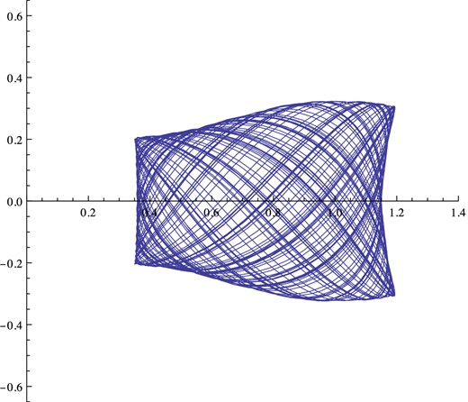
Figure 1.

Lissajoux figure traced by orbit 1 in a rotating meridional plane. Notice that only two lines cross at each point near the starting point (1,0.3). These are at angles to the axis corresponding to the starting v_z/v_R = 0.5 and the computed −0.44.

Open in new tab Download slide

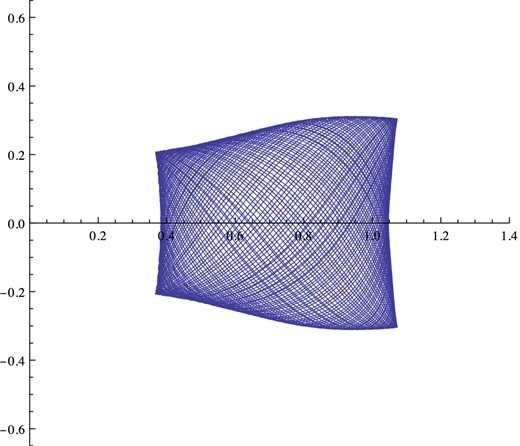
Figure 2.

Lissajoux figure traced by orbit 2 in a rotating meridional plane. Close to the starting point v_z/v_R = 0.5 or the computed −0.59.

Open in new tab Download slide

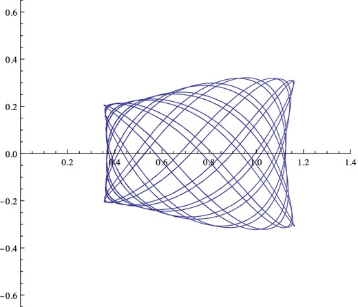
Figure 3.

Figure traced in a rotating meridional plane for an intermediate but resonant orbit. It has been computed for the same time as the other figures but the orbit retraces the same path rather than infilling the gaps.

Open in new tab Download slide

Table 2.

Open in new tab

Orbital returns n = number of orbit.

n	t	R	z
	v_R	v_z	v_R/v_z
1	0	1	0.3
	80	40	0.5
1	0.2083	0.991	0.298
	84	−37	−0.440
1	0.3596	0.992	0.298
	84	−37	−0.437
2	0	1	0.3
	50	25	0.5
2	0.0934	0.987	0.298
	−53	31	−0.595
2	0.1070	1.011	0.302
	44	−26	−0.589
2	0.1463	1.011	0.302
	−44	26	−0.594
2	0.2533	1.000	0.300
	−50	−25	0.498

n	t	R	z
	v_R	v_z	v_R/v_z
1	0	1	0.3
	80	40	0.5
1	0.2083	0.991	0.298
	84	−37	−0.440
1	0.3596	0.992	0.298
	84	−37	−0.437
2	0	1	0.3
	50	25	0.5
2	0.0934	0.987	0.298
	−53	31	−0.595
2	0.1070	1.011	0.302
	44	−26	−0.589
2	0.1463	1.011	0.302
	−44	26	−0.594
2	0.2533	1.000	0.300
	−50	−25	0.498

Table 2.

Open in new tab

Orbital returns n = number of orbit.

n	t	R	z
	v_R	v_z	v_R/v_z
1	0	1	0.3
	80	40	0.5
1	0.2083	0.991	0.298
	84	−37	−0.440
1	0.3596	0.992	0.298
	84	−37	−0.437
2	0	1	0.3
	50	25	0.5
2	0.0934	0.987	0.298
	−53	31	−0.595
2	0.1070	1.011	0.302
	44	−26	−0.589
2	0.1463	1.011	0.302
	−44	26	−0.594
2	0.2533	1.000	0.300
	−50	−25	0.498

n	t	R	z
	v_R	v_z	v_R/v_z
1	0	1	0.3
	80	40	0.5
1	0.2083	0.991	0.298
	84	−37	−0.440
1	0.3596	0.992	0.298
	84	−37	−0.437
2	0	1	0.3
	50	25	0.5
2	0.0934	0.987	0.298
	−53	31	−0.595
2	0.1070	1.011	0.302
	44	−26	−0.589
2	0.1463	1.011	0.302
	−44	26	−0.594
2	0.2533	1.000	0.300
	−50	−25	0.498

REFERENCES

An

J.

Evans

N. W.

2016

ApJ

816

35

Month:	Total Views:
December 2016	2
February 2017	5
March 2017	2
April 2017	3
June 2017	5
July 2017	4
November 2017	3
December 2017	1
January 2018	1
February 2018	10
July 2018	1
August 2018	1
February 2019	2
March 2019	1
May 2019	3
July 2019	5
August 2019	1
October 2019	8
November 2019	9
January 2020	8
February 2020	4
March 2020	5
April 2020	2
May 2020	3
June 2020	4
July 2020	5
August 2020	5
September 2020	1
October 2020	1
November 2020	1
December 2020	4
January 2021	2
February 2021	9
March 2021	9
April 2021	1
May 2021	2
June 2021	2
July 2021	5
August 2021	3
September 2021	3

Article Contents

Principal velocity surfaces in stellar dynamics Free

Abstract

1 INTRODUCTION

2 LOCAL INTEGRALS REVISITED

2.1 Potentials of the form |$\psi [{\boldsymbol r},\zeta (\lambda ,\mu )]$|

2.2 Potentials of the form |$\psi [{\boldsymbol r},\zeta (\lambda ),\eta (\mu )]$|

3 The existence of Eddington's principal velocity surfaces

4 TOO TRUE TO BE GOOD

5 A SIMPLE EXAMPLE

REFERENCES

APPENDIX A: CONFORMAL TRANSFORMATIONS IN FLAT 3-SPACE

Citations

Views

Altmetric

Email alerts

Astrophysics Data System

Citing articles via

Latest

Most Read

Most Cited

This Feature Is Available To Subscribers Only

Principal velocity surfaces in stellar dynamics