


Abstract
We examine subhaloes and galaxies residing in a simulated Λ cold dark matter galaxy cluster (|$M^{\rm crit}_{200}=1.1\times 10^{15}\,h^{-1}\,\mathrm{M}_{\odot }$|) produced by hydrodynamical codes ranging from classic smooth particle hydrodynamics (SPH), newer SPH codes, adaptive and moving mesh codes. These codes use subgrid models to capture galaxy formation physics. We compare how well these codes reproduce the same subhaloes/galaxies in gravity-only, non-radiative hydrodynamics and full feedback physics runs by looking at the overall subhalo/galaxy distribution and on an individual object basis. We find that the subhalo population is reproduced to within ≲10 per cent for both dark matter only and non-radiative runs, with individual objects showing code-to-code scatter of ≲0.1 dex, although the gas in non-radiative simulations shows significant scatter. Including feedback physics significantly increases the diversity. Subhalo mass and Vmax distributions vary by ≈20 per cent. The galaxy populations also show striking code-to-code variations. Although the Tully–Fisher relation is similar in almost all codes, the number of galaxies with 109 h− 1 M⊙ ≲ M* ≲ 1012 h− 1 M⊙ can differ by a factor of 4. Individual galaxies show code-to-code scatter of ∼0.5 dex in stellar mass. Moreover, systematic differences exist, with some codes producing galaxies 70 per cent smaller than others. The diversity partially arises from the inclusion/absence of active galactic nucleus feedback. Our results combined with our companion papers demonstrate that subgrid physics is not just subject to fine-tuning, but the complexity of building galaxies in all environments remains a challenge. We argue that even basic galaxy properties, such as stellar mass to halo mass, should be treated with errors bars of ∼0.2–0.4 dex.
1 INTRODUCTION
The complex environment of galaxy clusters provides a challenging and unique astrophysical laboratory with which to test our theories of cosmic structure formation and the processes that govern galaxy formation. The progenitors of these massive structures collapsed at high redshift, and so their present-day properties probe cosmic structure formation over a large fraction of the Universe's lifetime. A cluster's galaxy population is comprised of both those that have orbited within the dense, violent environment for several dynamical times and newly accreted field galaxies. Modelling these systems has been a great challenge given the enormous range in both spatial and temporal scales probed: from the local cooling of gas; conversion of gas to stars and injection of energy into the surrounding galactic medium from supernovae (SNe); to merger-driven star bursts and the powerful active galactic nucleus (AGN) outflows from massive galaxies that affect the large-scale intracluster medium.
Hydrodynamical simulations traditionally used either Lagrangian smoothed particle hydrodynamics (SPH) techniques (e.g. Gingold & Monaghan 1977; Lucy 1977; Monaghan 1992; Katz, Weinberg & Hernquist 1996; and see Springel 2010a for a review) or Eulerian grid-based solvers sometimes aided by adaptive mesh refinement (AMR) techniques (e.g. Cen & Ostriker 1992; Bryan et al. 1995; Kravtsov et al. 1997). Ideally, synthetic galaxies should be similar regardless of code or technique used. However, early comparisons of hydrodynamical N-body codes showed worrying differences between numerical approaches and even codes. The classic Santa Barbara Cluster Comparison Project (Frenk et al. 1999) compared the properties of a galaxy cluster formed in a non-radiative cosmological simulation using 12 then state-of-the-art mesh- and particle-based codes and found a large scatter in almost all bulk properties. The key difference confirmed in many other studies was the presence of a core in the radial entropy profile in mesh-based codes that was absent in SPH codes (e.g. Dolag et al. 2005; Voit et al. 2005; Mitchell et al. 2009).
Some of these differences can be attributed to the underlying technique used, whether SPH or mesh based. By its very nature, SPH can smooth out shocks, dampen subsonic turbulence and suppress fluid instabilities, at least for vanilla SPH (e.g. Okamoto et al. 2003; Agertz et al. 2007; Tasker et al. 2008). Mesh codes by construction are not Galilean invariant; consequently, results are sensitive to the presence of bulk velocities and significant advection errors can occur when fluids with sharp gradients move across cells in a manner unaligned with the grid, generating entropy spuriously through artificially enhanced mixing (e.g. Tasker et al. 2008; Wadsley, Veeravalli & Couchman 2008). AMR codes, which use flexible but necessarily ad hoc refinement criteria, have artefacts arising from the loss of accuracy at refinement boundaries. When coupled to gravity, this loss of accuracy leads to suppression of low-amplitude gravitational instabilities, which are seeds for cosmological structure formation, and violate energy and momentum conservation in the long-range forces whenever cells are refined or de-refined (e.g. O'Shea et al. 2005; Heitmann et al. 2008). Consequently, even for some simple non-radiative problems, classic Lagrangian and Eulerian codes will not converge to the same solution (e.g. Tasker et al. 2008; Hubber, Falle & Goodwin 2013). Modern codes have attempted to address some of the inherent issues with each method by the inclusion of higher order dissipative switches (e.g. Read, Hayfield & Agertz 2010), new SPH kernels, different SPH formulations (e.g. Hopkins 2013), subgrid physics in mesh codes (e.g. Maier et al. 2009) and hybrid methods (e.g. Springel 2010b; Hopkins 2014).
Comparisons are further complicated by the inclusion of uncertain baryonic physics governing galaxy formation. Although most codes attempt to reproduce the observed galaxy population, implementations of feedback physics vary and typically increases the code-to-code scatter. For instance, Scannapieco et al. (2012) found that different star formation (SF) and stellar feedback implementations lead to significant differences in the morphology, angular momentum and stellar mass of an isolated individual galaxy. Some of the differences are a simple result of different subgrid physics. Several studies have investigated tuning parameters using in subgrid models, clearly showing the need for some tuning (e.g. Haas et al. 2013a,b; Le Brun et al. 2014; Crain et al. 2015), although typically these models focus on varying parameters and not necessarily changing the subgrid implementation. Using the same SPH code, Duffy et al. (2010) showed that different subgrid models produced different baryonic distributions. However, different models need not necessarily produce different galaxy populations. Durier & Dalla Vecchia (2012) showed that two significantly different implementations of SN feedback in SPH codes, thermal and kinetic, do converge. In Scannapieco et al. (2012), the resulting disc galaxy was typically too concentrated but recent developments have shown that there are codes capable of producing more realistic disc galaxies (e.g. Vogelsberger et al. 2014; Feldmann & Mayer 2015; Murante et al. 2015; Schaye et al. 2015; Wang et al. 2015), motivating new comparison projects using individual galaxies such as the ongoing AGORA project (Kim et al. 2014).
The appearance of numerous modern SPH and mesh methods and significant developments in modelling the processes governing galaxy formation warrant a second look at synthetic clusters. Hence, 16 years later, the nIFTy comparison project aims to revisit the Santa Barbara comparison with new state-of-the-art hydrodynamical codes. The first paper in this series of comparisons (Sembolini et al. 2016) studied the bulk properties of the cluster environment using a single well-resolved cluster with 12 modern codes in pure N-body and adiabatic runs. This comparison clearly demonstrated the following.
The dark matter (DM) distribution in pure DM-only simulations show ≲20 per cent variation in the DM density profile.
In non-radiative runs, the variation in the DM density profile remains at ≲20 per cent, but the gas distribution shows variations of up to ∼100 per cent.
Newer SPH codes that use higher order kernels and more complex methods for modelling dissipative physics are in close agreement with mesh codes, with variations of ≲ 10 per cent, and more significantly these codes reproduce the entropy core seen in numerous mesh codes.
Clearly, the latest SPH codes have removed the long-standing problem of falling entropy profiles seen in Frenk et al. (1999).
In paper II (Sembolini et al. 2015) we examined the bulk properties of this same cluster in full physics runs. The inclusion of cooling, SF and feedback significantly increases the scatter between codes, with baryon and stellar fractions varying by 30 per cent. Furthermore, full physics removes between classic and modern SPH codes in regards to entropy profiles, i.e. full physics + classic SPH can produce entropy cores. Intriguingly, the dividing line in properties such as the temperature profile between codes is not the inclusion/absence of AGN, although AGN play an important role in limiting the effect of overcooling.
The next question, which we examine here, is whether codes reproduce not just the same overall cluster environment but also individual subhaloes and galaxies residing in the cluster. Here we examine multiple subhaloes/galaxies, and the change in the differences between codes with the inclusion of more complex physics, going from pure DM simulations to full feedback physics simulations. The goal is to identify the origins of any differences and determine relative ‘error’ bars for predictions from hydrodynamical simulations. This paper is organized as follows: we briefly describe the numerical methods in Section 2, highlighting the differences between the codes in Section 2.1. Our findings are presented in Sections 3 and 4, where we compare the subhalo/galaxy population as a whole and compare individual objects, respectively. We end with discussion in Section 5.
2 NUMERICAL METHODS
2.1 Codes
The initial nIFTy comparison project, as presented in Sembolini et al. (2016), included 13 codes – the cart variant of art, ramses, arepo, hydra and 9 variants of the gadget code. In this study as in Sembolini et al. (2015), we consider the subset of these codes in which full subgrid physics has been included: one AMR code, ramses, the moving mesh code, arepoand nine variants of the SPH gadget code. The subgrid physics included span the range from codes only including cooling and star formation (CSF) to those that also include supermassive black hole formation and associated AGN. Two codes, arepo and g3-music, have been run with variant subgrid physics. The salient features of each code are summarized in Table 1. A comprehensive summary of the approach taken to solving the hydrodynamic equations in each of these codes can be found in Sembolini et al. (2016) and a description of subgrid models in Sembolini et al. (2015) (and Appendix A).
A brief summary of the codes.
| Type | Code | SN | AGN | Comments |
|---|---|---|---|---|
| Mesh | ramses | |$\checkmark$| | Salpeter IMF; No SN feedback; thermal AGN; average metallicity. | |
| For more details, see Teyssier (2002), Teyssier et al. (2011) and Appendix A1.1. | ||||
| Moving mesh | arepo | |$\checkmark$| | |$\checkmark$| | Chabrier IMF; Springel & Hernquist (2003, hereafter SH03) SF; kinetic SN; thermal AGN; tracks nine individual elements. |
| Variant: arepo-sh that uses subgrid physics of g3-music (no AGN, SH03 SF, kinetic SN). | ||||
| For more details, see Vogelsberger et al. (2013, 2014) and Appendix A1.2. | ||||
| Classic SPH | g3-music | |$\checkmark$| | Salpeter IMF; SH03 SF; thermal and kinetic SN. | |
| Variant: g3-musicpi that uses modified kinetic feedback, metal-dependent cooling. | ||||
| For more details, see Sembolini et al. (2013) and Appendix A2.1. | ||||
| g3-owls | |$\checkmark$| | |$\checkmark$| | Chabrier IMF; Schaye & Dalla Vecchia (2008, hereafter SDV08) SF; kinetic SN; thermal AGN; cloudy (Ferland et al. 2013) (element-by-element) cooling; tracks 11 individual elements. | |
| For more details, see Schaye et al. (2010) and Appendix A2.1. | ||||
| g2-x | |$\checkmark$| | |$\checkmark$| | Salpeter IMF; SDV08 SF; thermal SN; thermal AGN, | |
| For more details, see Pike et al. (2014) and Appendix A2.1. | ||||
| Modern SPH | g3-x-art | |$\checkmark$| | |$\checkmark$| | Chabrier IMF; SH03 SF; kinetic SN; thermal ‘quasar’ and ‘radio’ AGN; tracks individual 16 elements; C4 Wendland kernel; artificial conduction to promote mixing; and time-dependent artificial viscosity. |
| For more details, see Beck et al. (2016) and Appendix A2.2. | ||||
| g3-pesph | |$\checkmark$| | Chabrier IMF; SH03 SF-based scheme with additional quenching in massive galaxies based on Rafieferantsoa et al. (2015); probabilistic kinetic SN-driven wind scheme; tracks four individual elements; pressure-entropy formulation of SPH of Hopkins (2013); HOCTS(n=5) kernel with 128 neighbours. | ||
| For more details, see Huang et al. (in preparation) and Appendix A2.2. | ||||
| g3-magneticum | |$\checkmark$| | |$\checkmark$| | Chabrier IMF; SH03 SF; thermal and kinetic SN feedback; thermal ‘quasar’ and ‘radio’ AGN; cloudy (Ferland et al. 2013) (element-by-element) cooling; tracks 11 individual elements; C6 Wendland kernel with 295 neighbours. | |
| For more details, see Hirschmann et al. (2014) and Appendix A2.2. |
We note that there are several unique combinations of subgrid physics modules: ramses has AGN feedback but NO supernova feedback; g3-pesph does not explicitly include AGN feedback but does have additional quenching for massive galaxies. Some codes also have full physics variants, most notably arepo, which has a model without AGN physics.
2.2 Data
The cluster we have used for the nIFTy comparison was drawn from the g3-music-2 cluster catalogue1 (Sembolini et al. 2013, 2014; Biffi et al. 2014), which consists of a mass-limited sample of resimulated haloes selected from the MultiDark cosmological simulation (Riebe et al. 2013). The MultiDark run simulated a 1 Gpc h−1 volume with 20483 DM particles in a |$(h,\Omega _{\rm m},\Omega _{\rm b},\Omega _\Lambda ,\sigma _8,n_{\rm s})=(0.7,0.27,0.0469,0.73,0.82,0.95)$| cosmology based on the best-fitting parameters to WMAP7+BAO+SNI data (Jarosik et al. 2011) using art (Kravtsov, Klypin & Khokhlov 1997) and the data are accessible online via the MultiDark Database.2
The g3-music-2 cluster catalogue was constructed by selecting all the objects with masses >1015 h−1 M⊙ at z = 0. These objects were then resimulated with eight times better mass resolution using the zooming technique described in Klypin et al. (2001). We focus on one cluster in particular, a moderately unrelaxed object with a mass of ≈1.1 × 10¹⁵ h−1 M⊙. The mass resolution of the nIFTy cluster in the pure DM simulations is mDM = 1.09 × 10⁹ h−1 M⊙, and in the gas physics runs, mDM = 9.01 × 10⁸ h−1 M⊙ and mgas = 1.9 × 10⁸ h−1 M⊙. Several sets of these simulations were produced by each code. Here, we focus on the so-called aligned runs, which are the set of simulations that result in approximately the same gravitational accuracy3 for those codes that have produced full physics runs, i.e. subgrid physics modelling the formation of stars (and possibly black holes).
2.3 Analysis
The output produced by the codes was all analysed using a unified pipeline. Haloes and subhaloes were identified and their properties calculated using velociraptor (aka stf; Elahi, Thacker & Widrow 2011, freely available at https://github.com/pelahi/VELOCIraptor-STF.git). This code first identifies haloes using a 3DFOF algorithm (3D Friends-of-Friends in configuration space; see Davis et al. 1985) and then identifies substructures using a phase-space FOF algorithm on particles that appear to be dynamically distinct from the mean halo background, i.e. particles which have a local velocity distribution that differs significantly from the mean, i.e. smooth background halo. Since this approach is capable of not only finding subhaloes, but also tidal streams surrounding subhaloes as well as tidal streams from completely disrupted subhaloes (Elahi et al. 2013), for this analysis we also ensure that a group is self-bound. Bound baryonic content of DM subhaloes is determined by associating gas and star particles with the closest DM particle in phase space belonging to a (sub)halo (see Knebe et al. 2013, for a study on identifying synthetic galaxies). The internal self-energy of the gas is taken into account when determining whether these particles are bound. If we were interested in identifying gas outflows from galaxies, we could relax this condition but for the purposes of this study, we require particles to be strictly bound. Galaxies are defined as any self-bound structure that contains 10 or more star particles, although for the purposes of this study we are generally interested in galaxies containing more than 100 star particles. We have not searched for self-bound star particle groups containing no DM, which are generally not produced by any of the codes, nor have we decomposed the stellar structures to search for bulges and discs.
3 The subhalo/galaxy population
We begin with the simplest comparison, the total number of (sub)haloes/galaxies within 2 h−1 Mpc of the cluster's centre is listed in Table 2 for each type of simulation, dark matter only (DM), non-radiative (NR) and full physics (FP) runs. When comparing the number of subhaloes, we could of course use the virial radius, |$R_{200}^c$|, which is ∼2 h−1 Mpc for all the simulations (g3-music has |$R_{200}^c=1.69\ h^{-1}\,{\rm Mpc}$|). However, since this radius does change from one simulation to the next by a few per cent, for simplicity we fix the radial cut to 2 h−1 Mpc.
Number of DM subhaloes and, for the full physics simulation, number of galaxies at z = 0 with DM mass MS ≥ 2 × 10¹⁰ h−1 M⊙ within 2 h−1 Mpc of the cluster centre. We define galaxies as objects that contain ≥10 star particles, that is stellar masses of M* ≥ 1.9 × 10⁹ h− 1 M⊙, assuming one generation of star particles is produced by a gas particle. We have highlighted values which significantly increase or decrease (by ≳ 25 per cent) going from DM→NR→FP.
| Code | Number of subhaloes | |||
|---|---|---|---|---|
| DM | NR | FP | Galaxies | |
| g3-music | 378 | 303 | 428 | 325 |
| g3-musicpi | ∥ | ∥ | 435 | 324 |
| ramses | 290 | 174 | 182 | 16 |
| arepo | 360 | 243 | 294 | 76 |
| arepo-sh | ∥ | ∥ | 341 | 220 |
| g3-x-art | 381 | 356 | 388 | 262 |
| g3-owls | 383 | 327 | 440 | 307 |
| g3-pesph | 371 | 328 | 425 | 273 |
| g2-x | 399 | 294 | 319 | 186 |
| g3-magneticum | 380 | 341 | 330 | 176 |
Note. ∥It means value is the same as row above.
We see that for the DM run, most codes have similar number of subhaloes to within Poisson errors.4 This pattern is also observed in the non-radiative simulations. arepo, the moving mesh code, is a moderate outlier. The main outlier is the sole adaptive mesh code, ramses, which has 20 per cent fewer DM subhaloes in the DM run. This number drops by ∼40 per cent (30 per cent) going from DM→NR for ramses (arepo), whereas in most SPH codes it decreases by only ∼10–20 per cent. The SPH outlier is g2-x, a classic SPH code, where the number of subhaloes decreases by 25 per cent.
The picture as always is more complex with the addition of feedback physics. Recall that certain codes, g3-music, arepo and g2-x have more than one flavour of full physics runs. In almost all cases, going from NR→FP, i.e. including cooling and feedback processes, increases the total number of subhaloes. Most SPH codes have even more in the FP runs than in the DM, the notable exceptions being g3-magneticum and g2-x, which behave similarly to arepo and ramses. Some of this increase is due to the resolution limit imposed: subhaloes must be composed of 20 or more particles, be they star particles, gas particles or DM particles. Thus in the FP runs, subhaloes with lower DM masses are counted if they also contain baryons. However, most of the increase occurs at masses above the resolution threshold imposed and is a result of the influence of baryons on DM.
The diversity in the number of subhaloes in the full physics runs is mirrored by the galaxy population. Most codes result in the cluster containing of the order of 200 galaxies, though this number ranges from 16 to 325. As our synthetic cluster is of similar to the Virgo cluster one would expect ∼60 massive galaxies (stellar masses M* ≳ 109.5), although the total number of cluster members is ∼1000 (Boselli et al. 2014). Caution should be used when directly comparing numbers is given the likely differences in merger histories between Virgo and our synthetic cluster and the complexity of estimating stellar masses from observations but we should expect similar numbers of galaxies. Typically, most codes produce more galaxies than one might naively expect. The two codes that stand out are the mesh codes, which have far fewer galaxies (and subhaloes) than the SPH codes. ramses has the fewest subhaloes and startlingly few galaxies, by far the lowest of any of the codes. arepo (Illustris physics) also has few galaxies, similar to that observed in Virgo, and a low fraction of subhaloes hosting galaxies. Its variant, arepo-sh has numbers similar to the SPH codes. Amongst the SPH codes, g3-magneticum has the smallest galaxy population and a low galaxy occupation fraction of ∼50 per cent. Other codes, such as g3-music and g3-owls, have occupation fractions of ∼80 per cent and ∼270–320 galaxies.
Perhaps the most relevant change to note is that due to different flavours of subgrid physics. The arepo-sh simulation, which has the same subgrid physics as g3-music, has a moderate change in the number of subhaloes but an enormous change in the galaxy population compared to arepo. The g3-music variant shows little change in the number.
3.1 Subhaloes
We next examine the cumulative mass and maximum circular velocity distributions shown in Figs 1 and 2, with the lower panels showing the ratio of the distribution from one code relative to the median calculated using all other codes. The mass distribution shows that all codes produce similar DM results. The only noticeable feature is the lack of small subhaloes in ramses, which matches the other codes reasonably well for subhaloes composed of ≳50 particles. The overall scatter for all codes using the gadget Tree-PM gravity solver is ≲10 per cent. The excess of MS ∼ 1012 h−1 M⊙ subhaloes in ramses is a result of these subhaloes residing outside our radial cut in most other simulations and a few subhaloes having slightly higher masses in ramses.
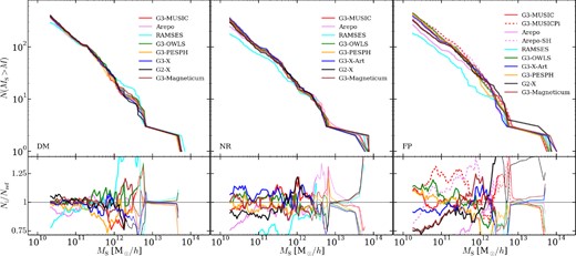
The subhalo cumulative mass function (top) and the difference between a given catalogue and the median calculated using all other catalogues (bottom). The thin lines in the residual plots correspond to where the catalogue's cumulative distribution has fewer than 10 subhaloes, i.e. the region where the statistical error is ≳10 per cent. Three types of simulations are shown: DM (left), NR (middle) and FP (right), respectively.

The general picture becomes worse with the inclusion of gas, although not significantly so despite the variety of approaches modelling gas. The scatter is typically ≲15 per cent. The key feature is that mesh codes, particularly ramses, have fewer objects. However, these codes do not exhibit precisely the same behaviour: arepo has fewer low-mass, poorly resolved objects, whereas ramses actually has a slightly flatter mass distribution across a wide range of masses. This lack of subhaloes in ramses is likely related to the known issue of lower small-scale power found in ramses compared to gadget at z > 1 where these objects should form (see fig. 1 of Schneider 2015).
Including feedback physics increases the scatter to ≳25 per cent for masses ≲1013 h−1 M⊙, although the form of the mass function is generally unchanged. The codes that bracket the overall variation are the g3-music variant and ramses.
The maximum circular velocity is less affected by tidal forces and differences in the position of a given subhalo relative to the host but is sensitive to changes in the central concentration of subhaloes (e.g. Onions et al. 2013). Therefore, we might expect less scatter arising from differences in the position of a subhalo and see biases in the central concentration that would not be evident in the mass distribution for well-resolved haloes where Vmax can be accurately measured. Like the mass distribution, the DM simulations agree with one another if one accounts for the difference in normalization, i.e. the residuals are flat. The non-radiative simulations also have little code-to-code scatter, with two exceptions. Both ramses and arepo have fewer subhaloes low Vmax subhaloes, and ramses has also flatter slopes (the residuals have a slight tilt).
Feedback physics causes the Vmax variation to be more pronounced than that seen in the mass. This variation is a result of appreciable amounts of baryons being moved around by the different cooling and feedback physics included by each code. g3-music subhaloes have higher circular velocities, whereas most other codes have steeper slopes with more low Vmax subhaloes. It is worth noting that arepo-sh, the variant not including AGN feedback (dashed lines), not only contains many more galaxies (see Table 2) but also contains subhaloes with high Vmax.
We examine the radial distribution via the enclosed number density n(rS < R) in Fig. 3, where rS is the radial distance a subhalo is from the cluster centre and R is the radial distance cut. For all simulation types, almost all codes produce the same overall shape, i.e. the residuals are flat though the normalization varies. Only in the very outskirts are significant differences apparent, which is not unexpected given that the DM profiles of the overall cluster agree to within ∼10 per cent. The DM simulations show the smallest amount of scatter and the FP simulations the most. The outlier in all simulation types is ramses, which drops faster than other codes. Note that the major jumps in the residuals seen in the core region are a result of differences in the positions of the few subhaloes identified deep within the host.

3.2 Baryons
Here, we focus on the baryonic component and the changes in the subhalo population resulting from the inclusion of adiabatic and full physics. Gas cooling can contract the core of a field DM halo (e.g. Gnedin et al. 2004), though the effect on a subhalo in the hot cluster environment is not as clear cut. Stripping of cold, low entropy gas contained in a subhalo as it falls into the cluster environment can counter adiabatic contraction. Codes treat mixing of low entropy gas differently, and consequently, the concentration of subhaloes should differ.
We highlight the differences in the Vmax distribution between the runs in Fig. 4. The ratio between NR and DM has a noticeable tilt for haloes with Vmax ≲ 200 km s−1 for the SPH simulations, with the two mesh codes, ramses and arepo, having less pronounced tilts. Adiabatic physics results in fewer subhaloes, less centrally concentrated subhaloes, increasing the number of low Vmax subhaloes over high Vmax subhaloes due to the efficient stripping of gas from small subhaloes.

In full physics runs, gas can cool and contract, centrally concentrating material and forming galaxies, although this can be completely counteracted by feedback physics (e.g. Abadi et al. 2010; di Cintio et al. 2011). The middle and bottom panels of Fig. 4, show that, for SPH codes, cooling and feedback physics has counteracted the expansion of subhaloes arising in the adiabatic runs, with g3-magneticum and both g3-music variants experiencing the largest change. Interestingly, the residual for ramses and arepo with AGN feedback are flat, i.e. feedback processes have balanced the contraction due to cooling, leaving haloes relatively unchanged from how they appear in pure DM simulations. Without AGN feedback, arepo-sh produces more high-Vmax subhaloes in line with the changes seen in g3-music.
The radial distribution shown in Fig. 5 is not significantly affected by additional physics except in the very centre. The inclusion of gas increases the number density within 500 h−1 kpc. This very central concentration is removed going from NR to FP, although full physics runs are still centrally biased compared to pure DM simulations, in agreement with Libeskind et al. (2010). Only ramses appears to have flat residuals.

We next examine baryon fractions in Fig. 6, where we show fb of all objects containing some amount of bound gas or stars. Focusing on the non-radiative simulations, the first notable feature is that the peak of the fb distribution is significantly less than Ωb/Ωm, the cosmic baryon fraction (solid vertical line). The hot cluster environment efficiently strips baryons away from subhaloes. Most codes have the same overall shape, a lognormal centred on fb ∼ 3 × 10⁻³. ramses may be an exception as it is not as strongly peaked as the other codes. There is also the suggestion of a second peak around the cosmic baryon fraction. These two distributions arise from galaxies that have resided in the cluster environment and newly infalling galaxies that have yet to be stripped, of which there are few within 2 h−1 Mpc.

Baryon fraction distribution (top) and the residuals relative to the median calculated in the same fashion as Fig. 1 (bottom subpanel). We show the NR and FP simulations in the top and bottom major panels, respectively. We indicate the cosmic baryon fraction Ωb/Ωm by a solid vertical line. Colour, line types are the same as in Fig. 1.
The bottom two panels of Fig. 6 show that gas CSF allows subhaloes to retain significantly higher baryon fractions in the cluster environment. There are even a few subhaloes with fb > Ωb/Ωm. These are typically undergoing some tidal disruption, which has momentarily increased fb. Key is the increase in the code-to-code scatter. arepo peaks and plateaus at fb ≳ 10−2, whereas most SPH codes have peaks at Ωb/Ωm, indicating that arepo's feedback processes are stronger and/or more efficient in moving material out of host subhalo. ramses is even more extreme, containing no subhaloes with fb close to the cosmic baryon fraction. Interestingly, g2-x has a broad baryon fraction distribution, with a less noticeable peak at Ωb/Ωm.
Fig. 6 showed that in non-radiative simulations, regardless of code, few subhaloes retain their gas (baryons) in the cluster environment. In Fig. 7, we show the gas fraction, fg, versus subhalo mass of all objects with non-negligible amounts in the upper subpanel and in the lower subpanel the probability that a subhalo of a given mass retains negligible amounts of gas (here we use fb < 10−2 based on Fig. 6). Reassuringly, most NR simulations produce similar distributions in the mass of subhaloes which are unable to retain significant gas fractions. Only subhaloes with M ≳ 2 × 10¹² h−1 M⊙ or ≳10−3 times the host cluster mass retain some gas. Note that both mesh codes are more likely to have massive gas-poor subhaloes than SPH codes with ramses again being an outlier.
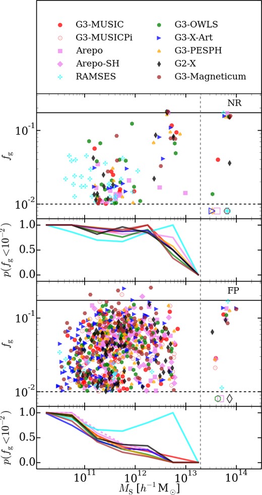
Gas fraction versus mass for NR (top two subpanels) and FP (bottom two subpanels) simulations. The cosmic baryon fraction is shown by a solid black horizontal line. In the bottom subpanels, we show the probability of a galaxy being stripped of all its gas, here assumed to be at fg ≤ 10−2, in a given mass bin for all objects of M ≤ 2 × 10¹³ h−1 M⊙ (dashed vertical line), above which there are very few objects. For those larger objects with fb ≤ 10−2, we plot them as open markers in the top panel. Colour, line types are the same as in Fig. 1, markers are indicated in the legend. For line legend see Fig. 1.
Code variations are also seen on an individual object basis. The most massive subhalo shown here has recently entered the cluster environment and consequently has fb ≈ Ωb/Ωm in all NR runs. However, the second largest subhalo, which lies closer to the cluster centre, has been completely stripped in the mesh or new SPH codes (open points), but retains some gas in the more classic SPH codes. This hint of bimodality between codes is not too surprising considering that studies of mesh and SPH codes using the blob test show that SPH codes increase the survival time of dense gas clumps exposed to a shock front or hot environment as a result of the artificially suppressed mixing present in the classic SPH formalism (e.g. Tasker et al. 2008). Generally, ramses and arepo have smaller fb than classic SPH codes, which is consistent with the quicker gas depletion of substructures found in arepo compared to gadget (Sijacki et al. 2012).
We should note that ramses has a few very low mass subhaloes with non-negligible gas fractions. These subhaloes reside at radii of ≳1500 h−1 kpc outside the hot cluster environment. The reason for this population is partially due to ramses's adaptive mesh, which is able to follow much smaller parcels of gas.
The lower two panels of Fig. 7 show that feedback physics changes the picture. Across all codes, only objects with M ≲ 1011 h−1 M⊙ are now devoid of gas, stripped by the combination of the cluster environment and internal feedback processes. The notable exception is ramses, which has a peak at much higher masses. This peak is partially a statistical fluke; there are only three subhaloes in this mass range, and they have all been stripped of gas. In general, the probability of being gas poor monotonically decreases with increasing mass, with arepo and particularly ramses having higher likelihoods than the other codes and g3-magneticum and g3-x-art having the lowest.
3.3 Galaxies
Hydrodynamical codes typically seek to reproduce the observed galaxy population, hence the first comparison to be made is the resulting stellar mass function of galaxies. However, as is evident from Table 2, different codes result in significantly different number of galaxies. Therefore, we examine both the galaxy stellar mass function (GSMF) and the normalized one, i.e. the probability of a galaxy having a stellar mass within a specific range, in Fig. 8. Note that we do not compare our GSMF to observations as there appears to be significant cluster-to-cluster variation (see fig. 12 of Boselli et al. 2011, for instance).
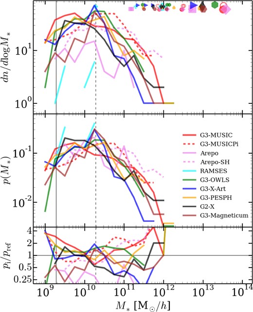
GSMF (top), normalized GSMF, i.e. probability of a galaxy having a mass within 0.25 dex of some mass M* (middle), and the residuals of the probability relative to the median calculated in the same fashion as Fig. 1 (bottom). We also plot the stellar mass of the BCG (includes the intercluster stars), and the three largest galaxies as large markers in the top panel (y ordinate is arbitrary value). The vertical solid line is at a mass of 10mgas (resolution limit for codes which have one generation of stars produced by a gas particle), and we also show a dashed line at 100mgas. Colour, line types and markers are the same as in Fig. 7. For marker legend see Fig. 7.
The stellar mass function shows large code-to-code scatter both for small and large galaxies, even when the differences in normalization are removed. Even the brightest central galaxy (BCG, including the intracluster light) differs by a factor of ≳4. The two mesh codes with AGN feedback, ramses and arepo, produce the smallest BCG, and arepo-shwithout AGN feedback produces the largest BCG. In fact, ramses severely stunts the growth to 1012 h−1 M⊙, a factor of 10 less massive than the next smallest BCG. Amongst the SPH codes, g3-music and g3-owls produce the largest, g3-x-art and g3-pesph the smallest, differing by a factor of ∼5.
This diversity is not simply due to different formulations of SPH or mesh codes evolving gas, the building blocks of stars, differently. For instance, the probability and number of low-mass galaxies in g2-x and g3-music differ by ≳2 for M* ≲ 5 × 10⁹ h− 1 M⊙, with g2-x having more. g3-music has much larger galaxies than g2-x. This is in spite of the fact that both use standard SPH; the differences lie in the subgrid physics. That is not to say that all codes disagree. g3-music and g2-x have monotonically decreasing stellar mass functions above masses of ∼2 × 10⁹ h−1 M⊙. Other codes typically produce stellar mass functions that are strongly suppressed for M* ≲ 1010 h− 1 M⊙, with g3-magneticum showing the strongest suppression. However, this turnover likely arises partially due to resolution effects and not solely due to SN feedback, as indicated by the fact that it occurs for masses corresponding to less than 100 star particles.
We can see the effects of different subgrid physics by looking at arepo and arepo-sh, that is, galaxies produced including/ignoring AGN physics. With the modified subgrid physics (specifically the lack of AGN feedback), arepo-sh is able to reproduce the BCG seen in g3-music and also has similar numbers of massive galaxies. In fact, it is more biased towards massive galaxies than g3-music. AGN physics is, however, not a precise dividing line between codes. g3-pesph, which does not included AGN feedback but has a modified SN feedback, has a BCG similar to g2-x and GSMF similar to g3-owls, AGN SPH codes.
The interplay between gas cooling and feedback is what transforms the (sub)halo mass function (Fig. 1) to the GSMF (Fig. 8). In small haloes, SN feedback should blow out gas from small haloes, whereas SF is suppressed in larger haloes by the energy injected into the surroundings by the supermassive black hole (AGN) residing in the (sub)halo centre. Despite the fact that subgrid physics in each code attempts to model these processes, the stellar mass to host halo mass relation, seen in Fig. 9, has large code-to-code scatter. Most codes have the same overall shape: M*/Mh decreases with increasing halo mass, with plateaus for Mh ≲ 1011 h−1 M⊙ and Mh ≳1012. However, g3-music (and g3-musicpi and arepo-sh) has an almost constant average M*/Mh relation and the efficiency of SF only seems to gradually decrease for much larger host haloes.5 Even for codes with similar M*/Mh shapes, the actual average M*/Mh for a given halo mass can vary by a factor of ∼4. For instance, galaxies in g2-x are far more DM dominated that those in g3-owls.
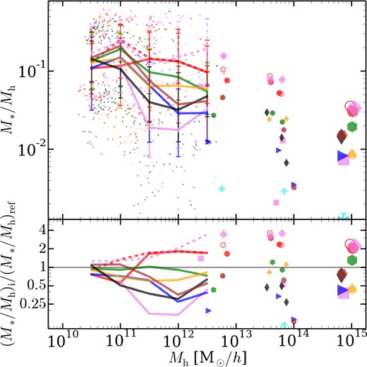
Stellar mass to host (sub)halo relation (top) and the residuals relative to the median calculated in the same fashion as Fig. 1 (bottom). In the top panel, we bin the data in host mass and plot median and 0.16,0.84 quantiles along with the data lying outside this range as small filled points. Similar to Fig. 8, we also plot the BCG and next three largest galaxies as points. Colour, line types and markers are the same as in Fig. 7. For legends see Figs 7 and 8.
Finally, we examine how well a common observational relation is reproduced, the Tully–Fisher/Faber–Jackson relations in Fig. 10. Here, we limit ourselves to a simple comparison, the maximum circular velocity as a function of stellar mass. We find that in contrast to the diversity seen in the other relations, there is little code-to-code scatter in the average relation. A galaxy with a mass M* will on average reside in a similar potential well ϕ ∝ GM/R regardless of code but the total mass associated with and size of that potential will vary from code to code. The only code that truly not follow the same slope and amplitude is ramses, where galaxies reside in far more massive subhaloes. g3-magneticum, g3-x-art and arepo also have low-mass galaxies residing in larger hosts than other codes, although to a lesser extent than ramses.
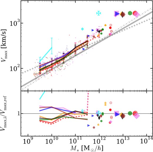
Relation between circular velocity and stellar mass (top) and the residuals relative to the median calculated in the same fashion as Fig. 1 (bottom), similar to Fig. 9. For reference, we also plot observational fits of Kassin et al. (2007, thick solid grey line), Dutton et al. (2011, thick dashed grey line) and Cortese et al. (2014, thick dash–dotted line) to field galaxies. For legends see Figs 7 and 8.
The relation produced by hydrodynamical codes differs from the observed relations shown in this figure; however, this is not completely unexpected given the environment probed here, a high-density cluster. Observations typically stack galaxies from a wide variety of environments. Furthermore, we have not split our galaxies into morphological types and estimated rotational or dispersive velocities from line-of-sight measurements within some radius, necessary if we wish to compare directly to observations. Overall, codes only differ from the observed relation significantly at high stellar masses. Only the BCGs lie off the observed trend; however, as these galaxies lie at the centre of the cluster, Vmax no longer probes the central galaxy but the overall cluster potential.
4 ONE-TO-ONE COMPARISONS
Section 3 shows that most codes reproduce the same bulk distribution when running DM or NR simulations. The question is whether this agreement masks a variation in an individual object's properties. The properties of an individual object that has experienced the same mass accretion history and dynamical environment should be the same. A quick glance at the previous section shows that all the codes reproduce the same large subhalo in terms of total mass. This subhalo is somewhat unique in that it has only been recently accreted around z ≈ 0.2 and lies at the outer edge of the cluster environment. The second most massive subhalo, which has resided for a longer period of time in the cluster environment, shows larger code-to-code variation. Here, we expand this line of comparison and search for counterparts between the subhalo catalogues produced by different simulation codes and compare their properties.
When comparing properties we could cross-correlate all catalogues with one another and compare codes relative to a virtual median object. However, not all objects are found in all catalogues. Moreover, using a median (or mean) implies a median model. What is this median model? If most codes were similar then that medial model is easily understood and variations about this median give rise to differences in properties, i.e. scatter. However, this is not the case as we have codes that have attempted to incorporate different feedback physics. As we are not only interested in the scatter between codes but also how different subgrid implementations affect galaxies, i.e. systematic differences, we use the g3-music catalogue as our reference, though any one could be used.
Before we compare properties, it is important to check whether this is a viable exercise by identifying subhaloes for which no counterpart is found. Recall that a counterpart is one which satisfies equation (1) with a merit of 0.2. If there are numerous missing subhaloes, then comparing individual objects is not informative as the codes have produced clusters with wildly different internal structures. We compare catalogues in Fig. 11, where we plot for every subhalo identified in the g3-music catalogue, the number of particles in a subhalo, its radial distance from the cluster centre and the fraction of other catalogues this subhalo exists in. Grey diamonds are subhaloes identified in all catalogues, black circles missing in all other catalogues and coloured squares for subhaloes identified in some catalogues.
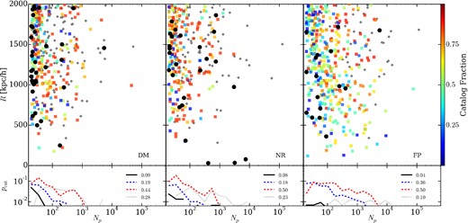
The distribution of ‘missing’ subhaloes, specifically the number of particles in the DM subhalo and its radial position from the centre of the host halo (top panel). We use the g3-music catalogue as our reference. Subhaloes that are missing in all other simulations are plotted as large black circles. Subhaloes that are missing in one or more catalogues but not all of them are plotted as filled squares, with the colour showing the fraction of catalogues it is missing in. Subhaloes identified in all catalogues are plotted as grey diamonds. In the lower panel, we show the probability distribution of missing subhaloes (solid black line), subhaloes found in fewer than 50 per cent of the catalogues (dashed blue line), subhaloes found in more than 50 per cent of the catalogues (dashed red line) and subhaloes found in all catalogues (dotted grey line), along with the total fraction of the catalogue in each of these subcategories. The three types of simulations are shown: DM (left), NR (middle) and FP (right) respectively.
If we pay particular attention to the subhaloes for which no counterpart is found, it is reassuring to know that most are composed of significantly less than 100 particles. Most large subhaloes, those composed of ≳500 particles, are present in all simulations, with a few interesting exceptions. The large subhalo identified in the DM-g3-music catalogue composed of ∼5 × 10³ particles at a radius of 1500 h−1 kpc is merging with the largest subhalo, also at 1500 h−1 kpc. Matches are identified in other catalogues but are not above the merit threshold used. This also applies to the object in the FP-g3-music catalogue. Similarly, the subhaloes in the NR-g3-music catalogue located at very small radii have matches but these less-than ideal matches are due to the difficulty of identifying subhaloes residing within the central regions of the halo hosts. Small differences in orbits will mean in some codes, different portions of the subhalo remain self-bound and are identified.
Given that ≲10 per cent of the subhalo population is ‘missing’ in the three types of simulations, one-to-one comparison of well-resolved subhaloes is meaningful. From here on, we will restrain our comparison to subhaloes composed of ≥100 particles in both catalogues. This limits our comparison to ≈105, ≈80 and ≈50 objects in the DM, NR and FP simulations, respectively.
4.1 Mass proxies
Fig. 12 shows the distribution of the ratio of a subhalo's bound mass and maximum circular velocity in one simulation to its counterpart in the g3-music catalogue for all well-resolved (Np ≳ 100) subhaloes. For almost all codes, the DM and NR runs have a ratio that follows a lognormal distribution. The typical variation is ∼20 per cent. The Vmax distribution has a smaller scatter, ≈10 per cent, not surprising since the central region usually defining Vmax is less affected by the tidal field of the cluster. The fact that all catalogues have similar variation suggests that this scatter is probably dominated by the differences in the exact orbits these subhaloes have taken in the highly non-linear cluster environment, rather than different hydrodynamical implementations. The main outlier is ramses, which primarily differs in the NR simulations. ramses produces smaller, less centrally concentrated subhaloes which are more susceptible to tidal disruption, hence the reason it has fewer subhaloes (see Table 2).
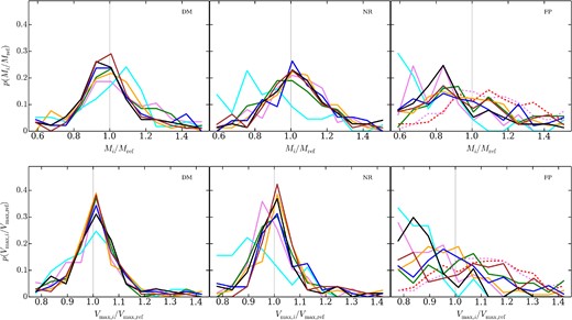
Ratio distribution of subhalo counter parts in simulation listed to those in the g3-music catalogue for mass (top) and Vmax (bottom) of the DM (left), NR (middle) and FP (right) simulations, respectively. Line styles and colours are the same as in Fig. 1. To guide the eye, we plot a solid grey vertical line at a ratio of 1 in both panels. For legend see Fig. 8.
Given the differences seen in Fig. 2 for the FP simulations, it is not surprising that even for subhaloes with a well-defined counterpart in the g3-music simulation, the ratio of Vmax shows systematic differences and vary greatly between codes. Feedback physics moves material out of cores of subhaloes, changing their circular velocity profiles significantly. What is somewhat unexpected is the variation in the mass. g3-music typically has more massive subhaloes than the other codes, and there is a great deal of variation which is not that readily apparent from Fig. 1.
4.2 Baryons
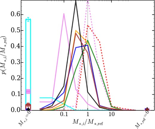
We compare baryon fractions in Fig. 13. When comparing the baryonic content of individual objects, we must account for the possibility that either the subhalo or its counterpart has been completely stripped of baryonic material, resulting in a ratio fb, i/fb, ref that spans (0, ∞). Therefore, we have binned objects where fb, i ≤ 0.1fb, ref and fb, i ≥ 10fb, ref separately in this figure. The non-radiative simulations have another issue: few objects contain non-negligible baryon fractions. For all the codes, ≈70 per cent of the cross-matched subhaloes have fb ≤ 10−2Ωb/Ωm in both catalogue. We ignore these stripped objects when comparing the ratio of the baryon fraction in Fig. 13.
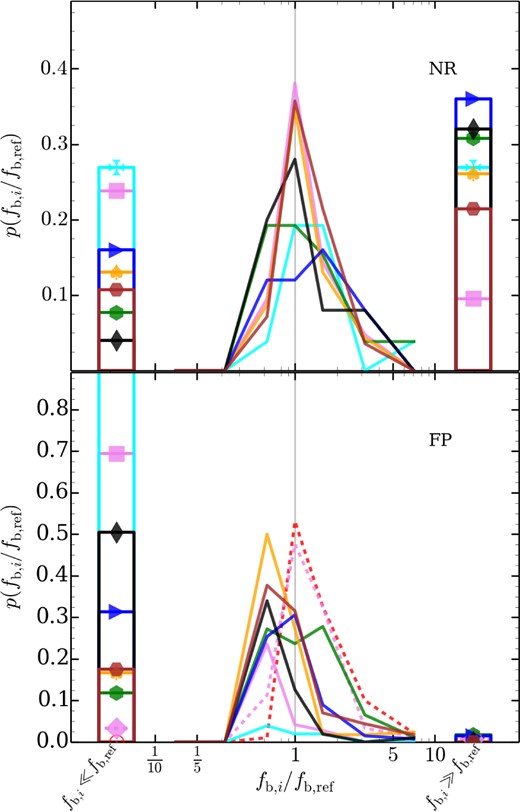
Baryon fraction comparison. Here, we plot a histogram of the fb ratio. We also plot two bins corresponding to subhaloes which contain negligible amounts baryons but have counterpart containing some, fb, i ≪ fb, ref, and vice versa, fb, i ≫ fb, ref. Line styles and colours are the same as in Fig. 1. For legend see Figs 7 and 8.
The first noticeable feature in the NR simulations is that for most codes there are two significant populations, the largest centred at fb, i/fb, ref ≈ 1. The major difference between codes lie which outlying bin contains a significant population. Subhaloes in arepo are more likely to have been stripped of their gas relative to g3-music. Conversely, most other codes are systematically less stripped, with g2-x and g3-x-art, a classic SPH and modern SPH code, having the largest systematic offset. Interestingly, ramses shows little bias in either direction.
In the FP runs, it appears that g3-music (and g3-musicpi) is the outlier, with subhaloes having higher baryon fractions. arepo-sh is the only other code with counterparts having similar baryon fractions. ramses, arepo and g2-x (both variants) have subhaloes biased to low fb. The question is whether g3-music's high baryon fractions are a consequence of it efficiently converting gas into stars, which are not subject to ram pressure or shocks, or whether these baryon-rich objects have simply managed to retain gas in instances where other codes have been stripped. Or perhaps the counterpart is more massive and therefore able to better hold on to its baryons. A closer examination of these objects reveals that their g3-music counterparts typically have the same mass (within 20 per cent) and contain both galaxies that have been stripped of or blown out all their gas and those that still have large reservoirs of fuel with which to form stars. Some of these galaxies even have gas fractions as high as Mg/Mb ∼ 0.5.
If we then focus on galaxies and their counterparts, we see in Fig. 14 significant systematic differences between codes in the stellar mass. arepo typically not only has galaxies that are an order of magnitude less massive, it has a significant population of empty subhaloes whose g3-music counterparts do host a galaxy. ramses is even more extreme. However, these are exceptions. Clearly for well-resolved subhaloes composed of ≥100 particles, if a galaxy is present in one code, it is present in another. The difference lies in the size. Typically, codes have less massive galaxies than g3-music, the exceptions being arepo-sh, which lacks AGN, and g3-musicpi. AGN feedback is not the sole reason for the difference as g3-pesph (no AGN) has smaller galaxies than g3-owls, which does have AGN feedback.
4.3 Galaxy/Subhalo diversity
We summarize the differences between subhaloes in a given simulation and their g3-music counterparts in Fig. 15. The logarithmic ratio, log (xi/xMUSIC), is typically well characterized by a normal distribution in the DM and NR runs, although some distributions have significant tails or broad peaks in the FP runs (see Fig. 12). Thus, we use the median, μ, and calculate an effective standard deviation, SD, using the 0.32 and 0.66 quantiles. Naturally, the median between a given catalogue and g3-music indicates whether systematic differences are present. Caution should be used in interpreting SD as it is the variation between g3-music and a given code, not the scatter between all codes. Note that here when comparing baryonic masses (and related quantities) we require that either the object or its reference counterpart have non-negligible amounts of gas/stars (depending on the comparison being made). For more complex properties such as spin, both must have non-negligible amounts.
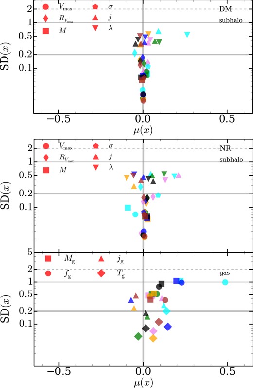
Properties comparison: we plot the median (μ) and standard deviation (SD) of the logarithmic ratio between the listed simulation and g3-music. Subhalo properties are Vmax, maximum circular velocity; |$R_{V_{\rm max}}$|, radius of Vmax; M, virial mass; σ, velocity dispersion; j, specific angular momentum; λ, the spin parameter from Bullock et al. (2001). Gas: Mg, gas mass; fg, gas fraction; jg, gas specific angular momentum; Tg, average temperature. We show several lines to guide the eye: a thick grey line at μ = 1 and SD = 0.2; and lines at SD = 1 and 2 dex. Marker colours are the same as in Fig. 7, see legend in Fig. 7.
First, examining the bulk subhalo properties in the DM runs, we see here that the mass and Vmax are well reproduced so long as SF and feedback physics are not included. There is not a significant systematic difference between codes and little scatter, with Vmax varying by ≲1 per cent. The velocity dispersion and |$R_{V_{\rm max}}$| are numerically converged for the non-full physics runs, with SD ≈ 0.2 dex. Angular momentum based quantities show large variations of up to 1 dex, primarily as j is affected by distant, marginally bound particles, and small differences in the exact position of a subhalo in one simulation to another will significantly contribute to the scatter. ramses is the only code to show some systematic offset, having subhaloes with marginally high spins.
We next present the NR runs. The subhalo properties are almost as well converged as those in the DM runs, with ramses the only code with some systematic differences, producing smaller, less concentrated subhaloes. The NR-gas panel of Fig. 15 shows that the gas distribution is less numerically converged, particularly the amount of gas, with an average variation of 0.25 dex. Some codes show greater code-to-code scatter of ∼1 dex (g3-x-art, g2-x, g3-owls). Most codes typically have more gas than g3-music. Interestingly, the gas temperature shows less scatter than the mass but the systematic differences between codes are more pronounced. The temperature bias does not appear to depend purely on numerical implementation as ramses and g3-x-art, two very different codes have higher temperatures. However, we do find that both mesh codes have higher angular momentum gas than SPH codes.
However, it is important to recall that the number of subhaloes with gas is small, so the μ and SD estimators suffer from small number statistics. Additionally, the Mg and fg ratios have a bimodal distribution since a subhalo can retain gas in one code but have been completely stripped in another. As we have used quantiles to estimate the mean and standard deviation, these subhaloes do not drastically skew these estimates (we treat them as containing one gas particle for the purposes of mass comparisons) and excluded when comparing other properties. Generally, ≈20–30 per cent of subhaloes fall into this category; therefore, the systematic differences and variance presented here are underestimates but the general features will not change.
In the full physics runs seen in Fig. 16, the scatter in the bulk properties of the galaxy/(sub)halo host have increased by ∼0.1 dex for Vmax and M, respectively. However, systematic differences are becoming noticeable, with Vmax in ramses and arepo being lower by ∼0.2 dex. The amount of gas has similarly increased scatter along with systematic differences. Both mesh codes differ significantly from the SPH results, being more gas poor by a factor of 2 for arepo and up to an order of magnitude for ramses. The scatter is also very high at ∼1 dex, whereas the SPH codes show ∼0.3 dex scatter.
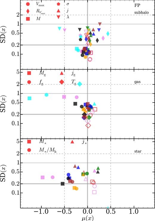
Similar to Fig. 15 but for the FP simulations. Also includes galaxy properties: M*, stellar mass, M*/Mh, stellar mass to halo mass; j*, stellar specific angular momentum. We also plot extra lines at μ = −0.5, 0.5, the x-axis limits in Fig. 15. Code variants g3-musicpi and arepo-sh are plotted as open points. Note that ramses only has a single well-resolved galaxy with a match in g3-music where the angular momentum can be measured and hence has SD = 0. To place this data point on the figure, we set SD = 0.02.
The galaxies stellar content shows a minimum of ∼0.15 dex scatter. More importantly, codes typically produce less massive galaxies than g3-music, with the two mesh codes with AGN being the most extreme. arepo's galaxies are 1 dex smaller. ramses's galaxies are 2.4 dex smaller (this lies off the figure) and has SD =0.43. Only g3-owls, arepo-sh and the g3-music variant itself produce similar galaxies to g3-music. The stellar angular momentum shows large code-to-code variation and scatter. For example arepo, g3-owls and g2-x galaxies relative to g3-music are more rotationally supported. The sole well-resolved ramses galaxy is also biased high. The other codes show that the overall picture is mixed as codes with/without AGN and modern and classic SPH codes have stellar distributions with similar angular momentum as g3-music.
We also calculate the effective standard deviation based on comparing objects to the median object. Recall that this median is calculated based on possibly incomplete list of catalogues as an object may not be present in all codes. Nevertheless this comparison, although it hides some systematic differences, is informative in estimating the code-to-code scatter. We find that for DM and NR runs the scatter for subhalo properties save angular momentum is similar to that seen in Fig. 15 at around ≲0.1 dex. The angular momentum related properties have higher scatter 0.2 dex scatter (lower than that calculated using g3-music as a reference). In the NR simulations, gas properties typically vary by 0.1–0.2 dex. Including SF and feedback physics increases the scatter for all properties, with subhalo quantities such as mass varying by ∼0.1 dex, gas properties varying by 0.2 dex and stellar properties vary by 0.2–0.4 dex.
5 DISCUSSION AND CONCLUSION
Hydrodynamical codes, regardless of specific numerical approach used, attempt to model (some of) the complex processes involved in forming a galaxy. In this paper, we have assessed how well hydrodynamic codes reproduce the same subhaloes and galaxies in a cluster environment using the nIFTy cluster data set. To address this goal, we have compared both the overall distribution of subhaloes and galaxies and compared individual objects.
We find that in DM only and non-radiative simulations, codes show 5–10 per cent scatter in the DM subhalo population and even on an individual object basis the scatter is only 0.1 dex for properties such as Vmax and mass.6 This is unsurprising considering the small amount of scatter in the DM distribution observed in Sembolini et al. (2016).
The differences lie in the baryonic component. In Sembolini et al. (2016), we found that even in NR runs, the gas entropy and density profiles of the cluster differed significantly from code to code, with mesh and modern SPH codes producing entropy cores whereas classic SPH codes produced ever falling entropy profiles. Here, we find that individual subhaloes show large variation in the baryonic fraction depending on the code used. The code-to-code scatter is 0.2–0.4 dex despite the overall similarity between codes in the likelihood of a subhalo being baryon poor. However, subhaloes do not show a strong separation between classic SPH and other codes.
The key result of this paper is that codes produce different galaxy populations and that the diversity is significant, despite all codes approaching galaxy formation in a similar fashion. Codes convert gas particles or cells into a ‘star’ particle when some criterion is satisfied, typically if a converging flow of gaseous material has high enough local densities and able to cool. This newly formed particle represents a star cluster, the basic galaxy building block. Star particles feed energy and metals back into the local environment. The issue is that these processes occur at unresolved scales, thus each code uses their own subgrid modules to model this complex process. Add to this mix, supermassive black holes, their growth by accretion and the associated injection of energy via AGN. Some codes include AGN feedback, some do not. Considering the variety of subgrid physics, some diversity is to be expected but perhaps not to the extent seen here. Even the bulk gas and stellar fractions of the entire cluster show marked differences, with gas and stellar fractions ranging from ∼0.12 to 0.18 and ∼0.01 to 0.05, respectively (Sembolini et al. 2015).
We find that the number of galaxies of a given stellar mass can vary by a factor of 4 in the cluster environment. The exception is ramses, which severely suppresses galaxy formation inside clusters, producing a paltry number of galaxies despite having no SN feedback. Among the other codes, arepo produces the fewest, followed by g3-magneticum, whereas g3-music and g3-owls produce the most.
Not only do the number of galaxies differ, but also codes do not produce the same stellar mass to halo mass relation. Codes with AGN physics have massive galaxies with much lower M*/Mh, yet some have higher M*/Mh values than g3-music for the lowest mass galaxies resolved here. Despite all this variety, codes generally produce the same effective baryonic Tully–Fisher (Faber–Jackson) relation, i.e. M*–Vmax relation, indicating that observations such as those of Bell & de Jong (2001) and Reyes et al. (2011) have limited use in pinning subgrid physics.
By comparing well-resolved individual objects between codes, we find that if a subhalo hosts a galaxy in one code, generally it will host a galaxy in other codes. The exceptions are the two mesh codes that include AGN, ramses and arepo, which have the lowest SF efficiencies. Of greater importance is that this synthetic galaxy will not have the same stellar mass across codes, despite having a similar merger and orbit history. First, we note that galaxies show large scatter of ∼0.2–0.5 dex in stellar mass, M*/Mh and stellar angular momentum. Secondly, there are significant systematic differences between codes. For example, galaxies in arepo are ∼1 dex less massive than those in g3-music.
The variety in synthetic galaxies and input subgrid physics is telling. Some codes with similar subgrid schemes, such as g2-x & g3-owls, which have similar SF and AGN but different initial mass functions (IMFs) and SN feedback and significantly different cooling curves (g2-x assumes solar metallicity), produce different numbers of galaxies. The number of galaxies here differ by 60 per cent, and distributions such as gas fractions and luminosity functions differ in shape. Changes in the cooling curve might account for some of these differences. Other examples of similar codes are g3-x-art and g3-magneticum. These two modern SPH codes have the same SF, IMF, similar AGN and differ in the SPH conduction scheme and significantly in the SN feedback scheme (g3-x-art has kinetic SN, g3-magneticum has both thermal and kinetic). Here, the differences are more subtle: the GSMFs have similar shapes but g3-magneticum has fewer low stellar mass galaxies likely due to stronger quenching from the addition of thermal SN feedback, resulting in g3-x-art having 50 per cent more galaxies with M* > 109 h− 1 M⊙.
Mesh codes at first glance are far less efficient than similar SPH codes at producing galaxies. arepo has similar subgrid schemes to the modern SPH code g3-x-art, yet has only 30 per cent of the galaxies that g3-x-art has. The galaxies in the arepo cluster are more likely to be stripped of gas, have lower stellar masses and do not follow the same GSMF, although they have a similar mass BCG (including intracluster stars). arepo also has galaxies with higher angular momentum than g3-x-art. This higher angular momentum difference appears to hinge on the AGN feedback scheme. arepo-sh, lacking AGN feedback, produces numbers much closer to that of g3-music, the only code lacking AGN feedback. Moreover, the distributions and even individual galaxies themselves are similar, although g3-music tends to produce a larger number of low stellar mass galaxies. The dependence of subgrid physics on the method used to evolve gas has been noted for the subgrid physics implemented (for instance the EAGLE simulations; Schaller et al. 2015; Schaye et al. 2015).
Many numerical studies show that AGN feedback can play an important role (e.g. McCarthy et al. 2010; Puchwein et al. 2010; Teyssier et al. 2011; Cui, Borgani & Murante 2014, although observational evidence may not be as clear cut, see Schawinski et al. 2014). However, the galaxy diversity seen between our suite of codes tells us that differences do not solely arise from the inclusion of AGN feedback. g3-owls, which has AGN, has similar mass galaxies to g3-music. Conversely, g3-pesph produces systematically lower mass galaxies than g3-owls yet it does not include AGN, although the use of a quenching model for massive galaxies in g3-pesph might mimic the statistical suppression of SF that AGN have.
In general, codes that reproduce the observed galaxy population in some respects, such as the luminosity function, in certain environments will need to be adjusted to reproduce galaxies in another environment. Therefore, subgrid physics as it stands is fine-tuned. The fact that subgrid physics requires tuning has been noted before (e.g. Haas et al. 2013a,b; Le Brun et al. 2014; Crain et al. 2015; Schaye et al. 2015). However, the similarity of galaxies produced by codes with different subgrid physics and differences between codes with similar schemes implies that the diversity and similarity are not solely a matter of fine-tuning a particular subgrid scheme. Rather current subgrid physics schemes do not fully capture the real processes governing galaxies.
In conclusion, our comparison suggests that the properties of any individual synthetic galaxy should be treated with errors bars of at least ∼0.2–0.4 dex.
The authors thank Joop Schaye for insightful comments. The authors also express special thanks to the Instituto de Fisica Teorica (IFT-UAM/CSIC in Madrid) for its hospitality and support, via the Centro de Excelencia Severo Ochoa Program under grant no. SEV-2012-0249, during the three week workshop ‘nIFTy Cosmology’ where this work developed. We further acknowledge the financial support of the University of Western 2014 Australia Research Collaboration Award for ‘Fast Approximate Synthetic Universes for the SKA’, the ARC Centre of Excellence for All Sky Astrophysics (CAASTRO) grant number CE110001020, and the two ARC Discovery Projects DP130100117 and DP140100198. We also recognize support from the Universidad Autonoma de Madrid (UAM) for the workshop infrastructure.
PJE is supported by the SSimPL programme and the Sydney Institute for Astronomy (SIfA), and Australian Research Council (ARC) grants DP130100117 and DP140100198. STK acknowledges support from STFC through grant ST/L000768/1. AK is supported by the Ministerio de Economía y Competitividad (MINECO) in Spain through grant AYA2012-31101 as well as the Consolider-Ingenio 2010 Programme of the Spanish Ministerio de Ciencia e Innovación (MICINN) under grant MultiDark CSD2009-00064. He also acknowledges support from the Australian Research Council (ARC) grants DP130100117 and DP140100198. He further thanks The Feelies for crazy rhythms. CP acknowledges support of the Australian Research Council (ARC) through Future Fellowship FT130100041 and Discovery Project DP140100198. WC and CP acknowledge support of ARC DP130100117. GY and FS acknowledge support from MINECO (Spain) through the grant AYA 2012-31101. GY thanks also the Red Española de Supercomputacion for granting the computing time in the Marenostrum Supercomputer at BSC, where all the MUSIC simulations have been performed. AMB is supported by the DFG Research Unit 1254 ‘Magnetisation of interstellar and intergalactic media’ and by the DFG Cluster of Excellence ‘Universe’. SB and GM acknowledge support from the PRIN-MIUR 2012 Grant ‘The Evolution of Cosmic Baryons’ funded by the Italian Minister of University and Research, by the PRIN-INAF 2012 Grant ‘Multi-scale Simulations of Cosmic Structures’, by the INFN INDARK Grant and by the ‘Consorzio per la Fisica di Trieste’. IGM acknowledges support from an STFC Advanced Fellowship. EP acknowledges support by the ERC grant ‘The Emergence of Structure during the epoch of Reionization’. JS acknowledges support from the European Research Council under the European Union's Seventh Framework Programme (FP7/2007-2013)/ERC grant agreement 278594-GasAroundGalaxies.
The authors contributed to this paper in the following ways: PJE organized and analysed the data, made the plots and wrote the paper. AK, GY and FRP organized the nIFTy workshop at which this program was completed. GY supplied the initial conditions. All the other authors, as listed in Section 2 performed the simulations using their codes. All authors have read and commented on the paper.
The simulations used for this paper have been run on a variety of supercomputers and are publicly available at the MUSIC website, http://www.music.ft.uam.es. MUSIC simulations were carried out on Marenostrum. arepo simulations were performed with resources awarded through STFCs DiRAC initiative. The authors thank Volker Springel for helpful discussions and for making arepo and the original gadget version available for this project. g3-pesph Simulations were carried out using resources at the Center for High Performance Computing in Cape Town, South Africa.
This research has made use of NASA's Astrophysics Data System (ADS) and the arXiv preprint server.
For more details on how these simulations were aligned, see Sembolini et al. (2016).
Despite the fact that all codes use the same initial conditions, an object in one code may lie just outside the radial cut used whereas in another code the object lies just within as a result of differences in the gravitational integration (see appendix in Sembolini et al. (2016) for related discussion on aligning codes). Moreover, the same object will experience slightly different tidal forces in each code and a subhalo that lies above the resolution threshold used in one code may have been stripped enough to lie below it in another.
Although the downturn in M*/Mh with decreasing Mh due to SN feedback at small halo masses is hinted at here, typically, this effect would most noticeable at host (sub)halo masses of ≲1010 h−1 M⊙, below the mass resolution used here.
Note that we only used codes that have full physics modules, mostly limiting our analysis to codes with similar Tree-PM gravity back-ends, the exception being ramses.
REFERENCES
APPENDIX A: CODES
A1 Mesh-based codes
A1.1 AMR
ramses(Teyssier, Perret):ramses is an AMR code that uses a directionally unsplit, second-order Godunov scheme with the HLLC Riemann solver to solve hydrodynamics and an adaptive particle mesh code to solve the Poisson equation. The grid is adaptively refined on a cell-by-cell basis, following a quasi-Lagrangian refinement strategy whereby a cell is refined into eight smaller new cells if its DM or baryonic mass grows by more than a factor of 8. Time integration is performed using an adaptive, level-by-level, time stepping strategy.
Cooling and heating: Gas cooling and heating is performed assuming coronal equilibrium with a modification of the Haardt & Madau (1996) UV background and a self-shielding recipe based on Aubert & Teyssier (2010). Hydrogen and helium cooling and heating processes are included following Katz et al. (1996), and metal cooling follows Sutherland & Dopita (1993). Here, the code also uses a temperature floor of 104 K to prevent spurious fragmentation of relatively poorly resolved galactic discs.
Star formation: SF is implemented as a stochastic process using a local Schmidt law as in Rasera & Teyssier (2006). The density threshold for SF was set to n* = 0.1H/cc, and the local SF efficiency per gas free fall time was set to 5 per cent.
Stellar population properties and chemistry: Each star particle is treated as a single stellar population (SSP) with a Chabrier (2003) IMF. Mass and metal return to the gas phase by core-collapse SNe only. A single average metallicity is followed during this process and advected in the gas as a passive scalar, to be used as an indicator of the gas metallicity in the cooling function.
Stellar feedback: In this project, no feedback processes related to the stellar population are used.
SMBH growth and AGN feedback: Supermassive black hole (SMBH) particles are represented by sink particles (Teyssier et al. 2011). The SMBH accretion follows Bondi accretion with the rate constrained by the instantaneous Eddington limit. When the gas density is larger than the SF density threshold the Bondi accretion rate is boosted (Booth & Schaye 2009). SMBH particles are evolved using a direct gravity solver, to obtain a more accurate treatment of their orbital evolution. SMBH particles more massive than 108 M⊙ are allowed to merge if their relative velocity is smaller than their pair-wise scale velocity. Less massive SMBH particles, on the other hand, are merged as soon as they fall within four cells from another SMBH particle. The AGN feedback used is a simple thermal energy dump with 0.1c2 of specific energy, multiplied by the instantaneous SMBH accretion rate.
A1.2 Moving mesh
arepo(Puchwein):arepo uses a Godunov scheme on an unstructured moving Voronoi mesh; mesh cells move (roughly) with the fluid. The main difference between arepo and traditional Eulerian AMR codes (such as art) is that arepo is almost Lagrangian and Galilean invariant by construction. The main difference between arepo and SPH codes (see the next subsection) is that the hydrodynamic equations are solved with a finite-volume Godunov scheme. The version of arepo used in this study conserves total energy in the Godunov scheme, rather than the entropy-energy formalism described in Springel (2010b). Detailed descriptions of the galaxy formation models implemented in arepo can be found in Vogelsberger et al. (2013) and Vogelsberger et al. (2014), but the key features can be summarized as follows.
Cooling and heating: Gas cooling takes the metal abundance into account. The metal cooling rate is computed for solar composition gas and scaled to the total metallicity of the cell. Photoionization and photoheating are followed based on the homogeneous UV background model of Faucher-Giguère et al. (2009) and the self-shielding prescription of Rahmati et al. (2013). In addition to the homogeneous UV background, the ionizing UV emission of nearby AGN is taken into account.
Star formation: The formation of stars is followed with a multiphase model of the interstellar medium (ISM) which is based on Springel & Hernquist (2003, hereafter SH03) but includes a modified effective equation of state above the SF threshold, i.e. above a hydrogen number density of 0.13 cm−3.
Stellar population properties and chemistry: Each star particle is treated as an SSP with a Chabrier (2003) IMF. Mass and metal return to the gas phase by asymptotic giant branch (AGB) stars, core-collapse SNe and Type Ia supernovae is taken into account. Nine elements are followed during this process (H, He, C, N, O, Ne, Mg, Si and Fe).
Stellar feedback: Feedback by core-collapse SNe is implicitly invoked by the multiphase SF model. In addition, we include a kinetic wind model in which the wind velocity scales with the local DM velocity dispersion (vwind ∼ 3.7σDM, 1D). The mass-loading is determined by the available energy which is assumed to be 1.09 × 1051 erg per core-collapse SN. Wind particles are decoupled from the hydrodynamics until they fall below a specific density threshold or exceed a maximum travel time. This ensures that they can escape form the dense ISM.
SMBH growth and AGN feedback: SMBHs are treated as collisionless sink particles. 105 M⊙ h−1 BHs are seeded into haloes once they exceed a mass of 5 × 10¹⁰ M⊙ h−1. The BHs subsequently grow by Bondi–Hoyle accretion with a boost factor of α = 100. The Eddington limit on the accretion rate is enforced in addition. AGN are assumed to be in the quasar mode for accretion rates larger than 5 per cent of the Eddington rate. In this case, 1 per cent of the accreted rest mass energy is thermally injected into nearby gas. For accretion rates smaller than 5 per cent of the Eddington rate, AGN are in the radio mode in which 7 per cent of the accreted rest mass energy is thermally injected into spherical bubbles (similar to Sijacki et al. 2007). Full details of the black hole (BH) model are given in Sijacki et al. (2015).
In addition to the main run, we have performed a simulation with simplified galaxy formation physics which allows a direct comparison to gadget simulations with the same baryonic physics. In this simulation, we account only for primordial cooling, photoheating by the UV background, SF with the SH03 model and kinetic wind feedback with a mass-loading of two times the SF rate and a wind velocity of ∼342 km s−1, essentially the subgrid physics of g3-music.
A2 SPH codes
A2.1 Classic
gadget3-music(Yepes, Sembolini): This is modified version of the gadget3 Tree-PM code that uses classic entropy-conserving SPH formulation with a 40-neighbour M3 kernel. The basic SH03 model was used. The variant, g3-musicpi, uses the same SPH formulation but different feedback (there are differences in how SN energy is distributed to surrounding SPH particles, the cooling function is metal dependent, it traces different metal species from Type Ia and SN-II separately and it switches off cooling around SN explosions; see Piontek & Steinmetz 2011).
Cooling and heating: Radiative cooling is assumed for a gas of primordial composition, with no metallicity dependence, and the effects of a background homogeneous UV ionizing field is assumed, following Haardt & Madau (2001).
Star formation: The SH03 model is implemented.
Stellar population properties and chemistry: A Salpeter (1955) IMF is assumed, with a slope of −1.35 and upper and lower mass limits of 40 and 0.1M⊙, respectively.
Stellar feedback: This has both a thermal and a kinetic mode; thermal feedback evaporates the cold phase within SPH particles and increases the temperature of the hot phase, while kinetic feedback is modelled as a stochastic wind (as in SH03) – gas mass is lost due to galactic winds at a rate |$\dot{M}_{\rm w}$|, which is proportional to the SF rate |$\dot{M}_{\ast }$|, such that |$\dot{M}_{\rm w} = \eta \dot{M}_{\ast }$|, with η = 2. SPH particles near the star-forming region will be subjected to enter in the wind in an stochastic way. Those particles impacted upon by the wind will be given an isotropic velocity kick of vw = 400 km s− 1 and will freely travel without feeling pressure forces up to 20 kpc distance from their original positions.
SMBH growth and AGN feedback: These processes are not included.
gadget3-owls(McCarthy, Schaye): The is a heavily modified version of gadget3 using a classic entropy-conserving SPH formulation with a 40-neighbour M3 kernel.
Cooling and heating: Radiative cooling rates for the gas are computed on an element-by-element basis by interpolating within pre-computed tables (generated with the cloudy code; cf. Ferland et al. 2013) that contain cooling rates as a function of density, temperature and redshift calculated in the presence of the cosmic microwave background and photoionization from a Haardt & Madau (2001) ionizing UV/X-ray background (further details in Wiersma, Schaye & Smith 2009a).
Star formation: SF follows the prescription of Schaye & Dalla Vecchia (2008, hereafter SDV08) – gas with densities exceeding the critical density for the onset of the thermogravitational instability is expected to be multiphase and to form stars (Schaye 2004). Because the simulations lack both the physics and numerical resolution to model the cold interstellar gas phase, an effective equation of state (EOS) is imposed with pressure P ∝ ρ4/3 for densities nH > n* where n* = 0.1 cm− 3. Gas on the effective EOS is allowed to form stars at a pressure-dependent rate that reproduces the observed Kennicutt–Schmidt law (Schmidt 1959; Kennicutt 1998) by construction.
Stellar population properties and chemistry: The ejection of metals by massive- (SNeII and stellar winds) and intermediate-mass stars (SNeIa, AGB stars) is included following the prescription of Wiersma et al. (2009b). A set of 11 individual elements are followed (H, He, C, Ca, N, O, Ne, Mg, S, Si and Fe), which represent all the important species for computing radiative cooling rates.
Stellar feedback: Feedback is modelled as a kinetic wind (Dalla Vecchia & Schaye 2008) with a wind velocity vw = 600 km s− 1 and a mass-loading η = 2, which corresponds to using approximately 40 per cent of the total energy available from SNe for the adopted Chabrier (2003) IMF. This choice of parameters results in a good match to the peak of the SFR history of the universe (Schaye et al. 2010).
SMBH growth and AGN feedback: Each BH can grow either via mergers with other BHs within the softening length or via Eddington-limited gas accretion, the rate of which is calculated using the Bondi–Hoyle formula with a modified efficiency, setting β = 2 as in Booth & Schaye (2009). The BH is forced to sit on the local potential minimum to suppress spurious gravitational scattering (Springel et al. 2005). Feedback is done by storing up the accretion energy (assuming ϵr = 0.1, ϵf = 0.15) until at least one particle can be heated to a fixed temperature of TAGN = 108 K (Booth & Schaye 2009).
gadget2-x(Kay): This is a modified version of the original gadget2 Tree-PM code that uses the classic entropy-conserving SPH formulation with a 40-neighbour M3 kernel. A detailed description of the code can be found in Pike et al. (2014), but its key features can be summarized as follows.
Cooling and heating: Cooling follows the prescription of Thomas & Couchman (1992) – a gas particle is assumed to radiate isochorically over the duration of its timestep. Collisional ionization equilibrium is assumed and the cooling functions of Sutherland & Dopita (1993) are used, with the metallicity Z = 0 to ignore the increase in cooling rate due to heavy elements. Photoheating rates are not included but the gas is heated to a minimum T = 104 K at z < 10 and nH < 0.1 cm−3.
Star formation: SF follows the method of SDV08; it assumes an equation of state for the gas with nH > 0.1 cm−3, with an effective adiabatic index of γeff = 4/3 for constant Jeans mass. Gas is converted to stars at a rate given by the Kennicutt–Schmidt relation (Schmidt 1959; Kennicutt 1998), assuming a disc mass fraction fg=1. The conversion is done stochastically on a particle-by-particle basis so the gas and star particles have the same mass.
Stellar population properties and chemistry: Each star particle is assumed to be an SSP with a Salpeter (1955) IMF.
Stellar feedback: A prompt thermal Type II SNe feedback model is used. This assumes that a fixed number, NSN, of gas particles are heated to a fixed temperature, TSN, with values of NSN = 3 and TSN = 1e7K chosen to match observed hot gas and star fractions (cf. Pike et al. 2014). Heated gas is allowed to interact hydrodynamically with its surroundings and radiate.
SMBH growth and AGN feedback: A variation on the Booth & Schaye (2009) model is used. BHs are seeded in friends-of-friends (FOF) haloes with more than 50 particles at z = 5, at the position of the most bound star or gas particle, which is replaced with a BH particle. The gravitational mass of the replaced particle is unchanged but an internal mass of 106 h−1M⊙ is adopted for the calculation of feedback. Each BH can grow either via mergers with other BHs within the softening length or via Eddington-limited gas accretion, the rate of which is calculated using the Bondi–Hoyle formula with a modified efficiency, setting β = 2 as in Booth & Schaye (2009). The BH is forced to sit on the local potential minimum, to suppress spurious gravitational scattering. Feedback is done by storing up the accretion energy (assuming ϵr = 0.1, ϵf = 0.15) until at least one particle can be heated to a fixed temperature of TAGN = 3 × 10⁸ K. This high temperature was chosen for high-mass clusters to match their observed pressure profiles – a lower temperature causes too much gas to accumulate in cluster cores because there is insufficient entropy to escape to larger radius.
A2.2 Modern
gadget3-x(Murante, Beck): This is a modified version of the non-public gadget3 that includes an artificial conduction term that largely improves the SPH capability of following gas-dynamical instabilities and mixing processes; a higher order Wendland C4 kernel (Dehnen & Aly 2012) to better describe discontinuities and reduce clumpiness instability; and a time-dependent artificial viscosity term to minimize viscosity away from shock regions. Pure hydrodynamical and hydro/gravitational tests on the performance of modified SPH scheme are presented in Beck et al. (2016).
Cooling and heating: Gas cooling is computed for an optically thin gas and takes into account the contribution of metals, using the procedure of Wiersma et al. (2009a), while a uniform UV background is included following the procedure of Haardt & Madau (2001).
Star formation: SF is implemented as in Tornatore et al. (2007), and follows the SF algorithm is that of SH03 – gas particles above a given density threshold are treated as multiphase. The effective model of SH03 describes a self-regulated, equilibrium ISM and provides a SF rate that depends upon the gas density only, given the model parameters.
Stellar population properties and chemistry: Each star particle is considered to be an SSP. We follow the evolution of each SSP, according to the Chabrier (2003) IMF. We account for metals produced in the SNeIa, SNeII and AGB phases, and follow 16 chemical species. Star particles are stochastically spawned from parent gas particles as in SH03, and get their chemical composition of their parent gas. Stellar lifetimes are from Padovani & Matteucci (1993); metal yields from Woosley & Weaver (1995) for SNeII, Thielemann et al. (2003) for SNeIa and van den Hoek & Groenewegen (1997) for AGB stars.
Stellar feedback: SNeII release energy into their surroundings, but this only sets the hot gas phase temperature and, as a consequence, the average SPH temperature of gas particles. SN feedback is therefore modelled as kinetic and the prescription of SH03 is followed (i.e. energy-driven scheme with a fixed wind velocity of 350 km s−1, wind particles decoupled from surrounding gas for a period of 30 Myr or until ambient gas density drops below 0.5 times the multiphase density threshold).
SMBH growth and AGN feedback: AGN feedback follows Steinborn et al. (2015). In the aforementioned model, SMBHs grow via Bondi–Hoyle like gas accretion (Eddington limited) with the model distinguishing between cold and hot component (see their equation 19). Here, only cold accretion is considered, using a fudge-factor αcold = 100 in the Bondi–Hoyle formula (i.e. αhot = 0). The radiative efficiency is variable, and it is evaluated using the model of Churazov et al. (2005). Such a model outputs separately the AGN mechanical and radiative power as a function of the SMBH mass and the accretion rate. Here, these are summed to give the resulting energy thermally to the surrounding gas with an AGN feedback/gas coupling efficiency of ϵfb = 0.5. The parameters of the hydro model were tuned using the tests presented in Beck et al. (2016) and those of the AGN model for reproducing observational scaling relations between SMBH mass and stellar mass of the host galaxies. No attempt was made to reproduce any of the observational properties of the intracluster medium. First results on the application of this code to simulations of galaxy clusters, including the reproduction of the cool core/non-cool core dichotomy, can be found in Rasia et al. (2015).
gadget3-pesph(February, Davé, Huang, Katz): This version of gadget uses the pressure-entropy SPH formulation of Hopkins (2013) with a 128 neighbour HOCTS (n = 5) kernel and the time-dependent artificial viscosity scheme of Morris & Monaghan (1997).
Cooling and heating: Radiative cooling using primordial abundances is modelled as described in Katz et al. (1996), with additional cooling from metal lines assuming photoionization equilibrium follows Wiersma et al. (2009a). A Haardt & Madau (2001) uniform ionizing UV background is assumed.
Star formation: SF follows the approach set out in SH03, where a gas particle above a density threshold of nH = 0.13 cm3 is modelled as a fraction of cold clouds embedded in a warm ionized medium, following McKee & Ostriker (1977). The SF rate obeys the Schmidt (1959) law and is proportional to |$n_{\rm H}^{1.5}$|, with the SF time-scale scaled to match the z = 0 Kennicutt (1998) relation. In addition, the heuristic model of Rafieferantsoa et al. (2015), tuned to reproduce the exponential truncation of the stellar mass function, is used to quench SF in massive galaxies. A quenching probability PQ, which depends on the velocity dispersion of the galaxy, determines whether or not SF is stopped in a given galaxy; if it is stopped, each gas particle eligible for SF first has its quenching probability assessed, and if it is selected for quenching then it is heated to 50 times the galaxy's virial temperature, which unbinds it from the galaxy.
Stellar population properties and chemistry: Each star particle is treated as an SSP with a Chabrier (2003) IMF throughout. Metal enrichment from SNeIa, SNeII and AGB stars are tracked, while four elements – C, O, Si and Fe – are also tracked individually, as described by Oppenheimer & Davé (2008).
Stellar feedback: SN feedback is assumed to drive galactic outflows, which are implemented using a Monte Carlo approach analogous to that used in the SF prescription. Outflows are directly tied to the SF rate, using the relation |$\dot{M}_{{\rm wind}} = \eta \times$|SFR, where η is the outflow mass-loading factor. The probability for a gas particle to spawn a star particle is calculated from the subgrid model described above, and the probability to be launched in a wind is η times the SF probability. If the particle is selected to be launched, it is given a velocity boost of vw in the direction of v × a, where v and a are the particle's instantaneous velocity and acceleration, respectively.
This is a highly constrained heuristic model for galactic outflows, described in detail in Davé et al. (2013), which utilizes outflows scalings expected for momentum-driven winds in sizeable galaxies (σ > 75 km s−1), and energy-driven scalings in dwarf galaxies. In particular, the mass-loading factor (i.e. the mass outflow rate in units of the SF rate) is η = 150 kms−1/σ for galaxies with velocity dispersion σ > 75 km s1 and η = 150 kms−1/σ2 for σ < 75 km s−1.
SMBH growth and AGN feedback: These processes are not included.
gadget3-magneticum (Saro): g3-magneticum is a modified version of gadget3 using a kernel based on the bias-corrected, sixth-order Wendland kernel (Dehnen & Aly 2012) with 295 neighbours. The code also incorporates a low-viscosity scheme to track turbulence (Dolag et al. 2005; Beck et al. 2016), gradients computed with a high-order scheme (Price 2012), thermal conduction is modelled isotropically at 1/20th of the Spitzer rate (Dolag et al. 2004) and a timestep limiting particle wake-up algorithm (Pakmor et al. 2012).
Cooling and heating: Cooling follows the prescription of Wiersma et al. (2009a) and photoionization from a Haardt & Madau (2001) ionizing UV/X-ray background. Radiative cooling rates for 11 elements (H, He, C, N, O, Ne, Mg, Si, S, Ca and Fe) are computed by interpolating within pre-computed tables (generated with the cloudy code; cf. Ferland et al. 2013)
Star formation: The SH03 model is implemented.
Stellar population properties and chemistry: Stars follow a Chabrier IMF. Chemical evolution follows Tornatore et al. (2007): metals are produced by SNII, by SNIa and by intermediate- and low-mass stars in the AGB. Metals and energy are released accounting for mass-dependent lifetimes with lifetimes according to Padovani & Matteucci (1993), metallicity-dependent stellar yields according to Woosley & Weaver (1995) for SNII, van den Hoek & Groenewegen (1997) for AGB stars and Thielemann et al. (2003) for SNIa.
Stellar feedback: The hot gas within the multiphase ISM model is heated by SNe and can evaporate the cold clouds. A certain fraction of massive stars (10 per cent) is assumed to explode as SNII triggering galactic winds with a mass-loading rate proportional to the SFR and a wind velocity of 350 km s−1.
SMBH growth and AGN feedback: SMBH and AGN feedback are based on Springel et al. (2005), Di Matteo, Springel & Hernquist (2005) and modifications of Sijacki et al. (2007), Fabjan et al. (2010), Hirschmann et al. (2014) and Dolag et al. (2015). SMBHs grow via Bondi–Hoyle accretion of gas or mergers. The accretion rate is limited to the Eddington rate and a characteristic boost factor of 100 is applied as only the accretion to large scale is captured. Unlike Springel et al. (2005) in which entire gas particles are accreted, here 1/4 of a gas particle's mass can be captured in an accretion event. During accretion events, 10 per cent of the accreted mass is converted into energy, 10 per cent of which is thermally coupled with gas within the smoothing length of the SMBH, weighted using the hydrodynamics SPH kernel. When the accretion rate drops below a threshold, it is assumed that there is a transition from a quasar mode to a radio mode of AGN feedback, and the feedback efficiency is enhanced by a factor of 4.
