


Abstract
We have simulated the formation of a galaxy cluster in a Λ cold dark matter universe using 13 different codes modelling only gravity and non-radiative hydrodynamics (ramses, ART, arepo, hydra and nine incarnations of gadget). This range of codes includes particle-based, moving and fixed mesh codes as well as both Eulerian and Lagrangian fluid schemes. The various gadget implementations span classic and modern smoothed particle hydrodynamics (SPH) schemes. The goal of this comparison is to assess the reliability of cosmological hydrodynamical simulations of clusters in the simplest astrophysically relevant case, that in which the gas is assumed to be non-radiative. We compare images of the cluster at z = 0, global properties such as mass and radial profiles of various dynamical and thermodynamical quantities. The underlying gravitational framework can be aligned very accurately for all the codes allowing a detailed investigation of the differences that develop due to the various gas physics implementations employed. As expected, the mesh-based codes ramses, art and arepo form extended entropy cores in the gas with rising central gas temperatures. Those codes employing classic SPH schemes show falling entropy profiles all the way into the very centre with correspondingly rising density profiles and central temperature inversions. We show that methods with modern SPH schemes that allow entropy mixing span the range between these two extremes and the latest SPH variants produce gas entropy profiles that are essentially indistinguishable from those obtained with grid-based methods.
INTRODUCTION
Galaxy clusters are the largest virialized objects in the Universe and, as such, provide both an important testbed for our theories of cosmological structure formation and a challenging laboratory within which to study the fundamental physical processes that drive galaxy formation and evolution. The overdense regions that contain clusters in the present-day Universe were the first to collapse and virialize in the early Universe, and so our theories must predict their assembly history over a large fraction of the lifetime of the Universe (see Allen, Evrard & Mantz 2011; Kravtsov & Borgani 2012, for a recent review). At the same time, galaxies in the cores of clusters have orbited within the often violently growing cluster potential over many dynamical times, while the broader cluster galaxy population is continually replenished by the infall of galaxies from the field.
Computer simulations are now well established as a powerful and indispensable tool in the interpretation of astronomical observations (see for instance Borgani & Kravtsov 2011). Early N-body simulations (White 1976; Fall 1978; Aarseth, Turner & Gott 1979), which included the gravitational effects of dark matter only, were vital in interpreting the results of galaxy redshift surveys and unveiling the large-scale structure of the Universe, and subsequently in resolving structure in the non-linear regime of dark matter halo formation. The focus of modern simulations has now shifted to modelling galaxy formation in a cosmological context (see Borgani & Kravtsov 2011 for a recent review), incorporating the key physical processes that drive galaxy formation – such as the cooling of a collisional gaseous component (e.g. Pearce et al. 2000; Muanwong et al. 2001; Davé, Katz & Weinberg 2002; Kay et al. 2004; Nagai, Kravtsov & Vikhlinin 2007; Wiersma, Schaye & Smith 2009), the birth of stars from cool overdense gas (e.g. Springel & Hernquist 2003; Schaye & Dalla Vecchia 2008), the growth of black holes (Di Matteo, Springel & Hernquist 2005) and the injection of energy into the interstellar medium by supernovae (e.g. Metzler & Evrard 1994; Borgani et al. 2004; Davé, Oppenheimer & Sivanandam 2008; Dalla Vecchia & Schaye 2012) and powerful active galactic nuclei (AGN) outflows (e.g. Thacker, Scannapieco & Couchman 2006; Sijacki et al. 2007, 2008; Puchwein, Sijacki & Springel 2008; Booth & Schaye 2009). These processes span an enormous dynamic range, both spatial and temporal, from the sub-pc scales of black hole growth to the accretion of gas on to Mpc scales from the cosmic web. Galaxy clusters offer an ideal testbed for the study of these processes and their complex interplay, precisely because their enormous size encompasses the range of scales involved. For this reason, the study of galaxy formation and evolution in cluster environments occupies a fundamental position in observational and numerical astrophysics.
These results have been confirmed subsequently by several studies (Dolag et al. 2005; O'Shea et al. 2005; Voit, Kay & Bryan 2005; Wadsley, Veeravalli & Couchman 2008; Mitchell et al. 2009; Valdarnini 2012). For example, Wadsley et al. (2008) and Mitchell et al. (2009) suggested that the discrepancy owes also to the artificial surface tension and the associated lack of multiphase fluid mixing in classic SPH, while similar conclusions have been reached by Sijacki et al. (2012) when comparing the moving mesh code arepo of Springel (2010) with classic SPH, using p-gadget3 with the entropy conserving SPH version of Springel & Hernquist (2002). Interestingly, in their recent study, Power, Read & Hobbs (2014) have shown that SPHS (Read & Hayfield 2012), an extension of SPH that improves the treatment of mixing by means of entropy dissipation, produces constant entropy cores in non-radiative galaxy cluster simulations that are consistent with the results of the adaptive mesh refinement (AMR) code ramses (Teyssier 2002). Both Wadsley et al. (2008) and Maier et al. (2009) report entropy cores in runs that incorporate subgrid models for turbulence. These results suggest that modern SPH codes can overcome the problems first reported in SB99 and subsequently in Agertz et al. (2007). It is worth noting that it is not obvious that mesh-based codes necessarily recover the correct form for the entropy profile. For example, Springel (2010) reports significant variation in the entropy profile for the same AMR code (enzo) that is particularly sensitive to choice of refinement criteria. More generally, differences are apparent when comparing AMR results to that of the moving mesh code arepo; Springel (2010) reports an entropy core that is significantly lower than that found in AMR codes (e.g. compare fig. 45 of Springel 2010 with fig. 18 of SB99 or fig. 5 of Voit et al. 2005).
In this work – emerging out of the ‘nIFTy cosmology’ workshop1 – we revisit the idea of the Santa Barbara Cluster Comparison Project 15 yr later. We take five modern cosmological simulation codes (with one of them taken in eight different flavours, for a total of 12 different codes) and study the formation and evolution of a large galaxy cluster (with final mass |$M_{\rm 200}^{\rm crit} \simeq 1.1 \times 10^{15}$| M⊙). First we perform blind dark matter-only simulations with the favoured parameter sets of each group. The results from these show the typical scatter that is expected for currently published works in this area. We then use a common parameter set to align our gravitational framework before continuing to study non-radiative gas simulations. This allows us to focus solely on the differences between the models that arise due to the different hydrodynamical implementations. This also permits us to cleanly study the formation (or not) of a gas entropy core.
The rest of this paper is organized as follows. in Section 2 we briefly describe the 12 methods used in this study and supply tables listing parameter choices. In Section 3 we describe how our initial conditions were generated and chosen. The main results are presented in Section 4, which discusses the dark matter-only simulations, and in Section 5, which presents the results from the non-radiative simulations. We discuss convergence and scatter among the different codes in Section 6. We summarize out results in Section 7. We present additional supporting material in Appendix A.
THE CODES
The numerical codes used for this project can be divided into two main groups: mesh-based and SPH codes. The mesh-based codes used in this work are ramses (Teyssier 2002), art (Rudd, Zentner & Kravtsov 2008) and arepo (Springel 2010): the first two use Eulerian hydrodynamics while arepo uses a moving unstructured mesh and can be considered almost Lagrangian. SPH codes use Lagrangian hydrodynamics: we study hydra (Couchman, Thomas & Pearce 1995) and nine different versions of gadget (Springel 2005). Among the SPH codes we can distinguish classic and modern forms. We define modern variants as those which adopt an improved treatment of discontinuities.
The various codes employ different techniques to solve the evolution equations for a two-component fluid of dark matter and non-radiative gas coupled by gravity. To calculate gravitational forces, ramses and art use AMR while arepo and gadget are based on the TreePM method. hydra uses an ap3m approach. Hydrodynamical forces are treated in the following ways: by means of SPH in gadget and hydra, using a Voronoi mesh in arepo, and using Eulerian AMR in ramses.
There follow short summaries detailing the specifics of each simulation code contributing to this comparison and the authors responsible for running each method. We focus on key differences and novel aspects. Generalized descriptions of the individual codes can be found in their respective methods papers, listed in Table 1. Table 2 summarizes the key numerical parameters used by each team.
List of all the simulation codes participating in the nIFTy cluster comparison project, including reference and gravity algorithm adopted.
| Code name | Reference | Gravity model |
|---|---|---|
| ramses | Teyssier (2002) | AMR |
| art | Rudd et al. (2008) | AMR |
| arepo | Springel (2010) | TreePM |
| gadget: | Springel (2005) | TreePM |
| g2-anarchy | Dalla Vecchia et al. (in preparation) | |
| g3-x-art | Beck et al. (2016) | |
| g3-sphs | Read & Hayfield (2012) | |
| g3-magneticum | Hirschmann et al. (2014) | |
| g3-pesph | Huang et al. (in preparation) | |
| g3-music | Sembolini et al. (2013) | |
| g3-owls | Schaye et al. (2010) | |
| g2-x | Pike et al. (2014) | |
| hydra | Couchman et al. (1995) | ap3m |
Key numerical parameters used for each run. Columns 2 and 3 list values for the Plummer-equivalent softening lengths for the dark matter particles in physical (not comoving) units (kpc), columns 4 and 5 list the same but for the gas particles (where present) and column 6 lists the number of FFT cells along each side of the box. We use the label ‘Adp’ when adaptive force resolution is used.
| Code name | ϵDM | |$\epsilon ^{\rm max}_{\rm DM}$| | ϵgas | |$\epsilon ^{\rm max}_{\rm gas}$| | NFFT |
|---|---|---|---|---|---|
| ramses | 11.0 | 11.0 | 11.0 | 11.0 | 256 |
| art | Adp | Adp | Adp | Adp | 256 |
| arepo | 33.0 | 5.5 | Adp | Adp | 512 |
| g2-anarchy | 20.0 | 5.0 | 20.0 | 5.0 | 512 |
| g3-x-art | 8.0 | 6.0 | 8.0 | 6.0 | 512 |
| g3-sphs | 5.0 | 5.0 | Adp | Adp | 1024 |
| g3-magneticum | 11.25 | 3.75 | 3.75 | 3.75 | 256 |
| g3-pesph | 5.0 | 5.0 | 5.0 | 5.0 | 256 |
| g3-music | 8.0 | 6.0 | 8.0 | 6.0 | 512 |
| g3-owls | 9.77 | 5.0 | 9.77 | 5.0 | 1024 |
| g2-x | 24.0 | 6.0 | 24.0 | 6.0 | 512 |
| hydra | Adp | 5.0 | Adp | 5.0 | 512 |
Mesh-based codes
ramses (Perret, Teyssier)
ramses is an AMR code. For fluid dynamics a directionally unsplit, second-order Godunov scheme with the HLLC Riemann solver is used. The N-body solver is an adaptive particle mesh code, for which the Poisson equation is solved using the multigrid technique. The grid is adaptively refined on a cell-by-cell basis, following a quasi-Lagrangian refinement strategy whereby a cell is refined into eight smaller new cells if its dark matter or baryonic mass grows by more than a factor of 8. Time integration is performed using an adaptive, level-by-level, time stepping strategy. Parallel computing is based on the MPI library, with a domain decomposition set by the Peano–Hilbert space filling curve.
art (Nagai, Lau, Nelson)
art (Adaptive Refinement Tree, ART) is an N-body plus hydrodynamics code with adaptive mesh refinement developed by Kravtsov, Klypin & Khokhlov (1997). The computational grid is refined based on the oct-tree structure: when a property of a given grid cell, e.g. density, exceeds certain predefined threshold, the cell is refined into eight smaller child cells. We solve the Poisson equation using FFT on the base grid, while for each refinement level we employ a multilevel relaxation method. The code solves the inviscid fluid dynamical equations using a second-order accurate Godunov method with piecewise-linear reconstructed boundary states and the exact Riemann solver of Colella & Glaz (1985). The version of the code (Rudd et al. 2008) used for this work has been parallelized for distributed machines using MPI and features a flexible time-stepping hierarchy.
arepo (Puchwein)
arepo uses a Godunov scheme on an unstructured moving Voronoi mesh. The mesh cells move (roughly) with the fluid. The main differences to Eulerian AMR codes consist in that arepo is almost Lagrangian and it is Galilean invariant by construction; furthermore, arepo has automatic refinement for hydrodynamics and gravity and uses a TreePM gravity solver. The main difference to SPH codes is that the hydrodynamic equations are solved with a finite-volume Godunov scheme. In this work, we always use the total energy as a conserved quantity in the Godunov scheme rather than the entropy–energy formalism described in Springel (2010).
SPH codes
g2-anarchy (Dalla Vecchia)
g2-anarchy is an implementation of gadget2 employing the pressure-entropy SPH formulation derived by Hopkins (2013). The artificial viscosity switch has been implemented following Cullen & Dehnen (2010), whose algorithm allows precise detection of shocks which avoids excessive viscosity in pure shear flows. g2-anarchy uses a purely numerical switch for entropy diffusion similar to the one of Price (2008), but without requiring any diffusion limiter. The kernel adopted is the C2 function of Wendland (1995) with 100 neighbours, with the purpose of avoiding particle pairing (as suggested by Dehnen & Aly 2012). The time stepping adopted is described in Durier & Dalla Vecchia (2012).
g3-x-art (Murante)
g3-x-art is an advanced version of gadget3 incorporating the Wendland kernel functions (Dehnen & Aly 2012) with 200/295 neighbours, artificial conductivity to promote fluid mixing following Price (2008) and Tricco & Price (2013), but with an additional limiter for gravitationally induced pressure gradients, a time-step limiting particle wake-up scheme (Pakmor et al. 2012) and a high-order scheme for gradient computation (Price 2012), shock detection and artificial viscosity similar to Cullen & Dehnen (2010) and Hu et al. (2014). A companion paper (Beck et al. 2016) presents an improved hydrodynamical scheme and its performance in a wide range of test problems. In order to clearly illustrate the changes due to an improved SPH implementation within an identical code, this variant of gadget has also been run with a cubic spline kernel, 64 neighbours, low-order viscosity and a shear flow limiter (Balsara 1995) and no conduction. Results from this version, g3-x-std, are included on the radial plots below but omitted from the panel figures as the results are in all cases essentially indistinguishable from the other gadget implementations of classic SPH.
g3-sphs (Power)
g3-sphs was developed to overcome the inability of classic SPH to resolve instabilities. It has been implemented in the gadget3 code. The key differences with respect to standard gadget3 are in the choice of kernel and in dissipation. Rather than the cubic spline kernel, g3-sphs uses as an alternative either the HOCT kernel with 442 neighbours or the Wendland C4 kernel with 200 neighbours. A higher order dissipation switch detects, in advance, when particles are going to converge. If this happens, conservative dissipation is switched on for all advected fluid quantities. The dissipation is switched off again once particles are no longer converging. This ensures that all fluid quantities are single valued throughout the flow by construction.
g3-magneticum (Saro)
g3-magneticum is an advanced version of gadget3. In this non-radiative version, a higher order kernel based on the bias-corrected, sixth-order Wendland kernel (Dehnen & Aly 2012) with 295 neighbours is included. The code also incorporates a low viscosity scheme to track turbulence as originally described in Dolag et al. (2005) with improvements following Beck et al. (2016), which uses a high-order scheme (Price 2012) to compute velocity gradients. Thermal conduction is modelled isotropically at 1/20th of the Spitzer rate (Dolag et al. 2004). At last, it uses a particle wake-up algorithm (Pakmor et al. 2012; Dolag, private communication) for a more accurate time integration.
g3-pesph (February)
g3-pesph is an implementation of gadget3 with pressure-entropy SPH (Hopkins 2013) which features special galactic wind models. The SPH kernel is an HOCTS (n = 5) B-spline with 128 neighbours. The time-dependent artificial viscosity is that of Morris & Monaghan (1997).
g3-music (Yepes)
The original MUSIC runs (g3-music) were completed with the gadget3 code, based on the entropy-conserving formulation of SPH (Springel & Hernquist 2002). gadget3 employs a spline kernel (Monaghan & Lattanzio 1985) and parametrized artificial viscosity following the model described by Monaghan (1997).
g3-owls (McCarthy)
The g3-owls simulations were run using a version of gadget3 which was significantly modified to include new subgrid physics for radiative cooling, star formation, stellar feedback, black hole growth and AGN feedback, developed as part of the OWLS/cosmo-OWLS projects (Schaye et al. 2010). Standard entropy-conserving SPH (Le Brun et al. 2014) was used with 48 neighbours.
g2-x (Kay)
g2-x is a modified version of the gadget2 code, using the TreePM gravity solver and standard entropy-conserving SPH. It includes a number of subgrid modules to model metal-dependent radiative cooling, star formation and feedback from supernovae and AGN.
hydra (Thacker)
hydra-omp (Thacker & Couchman 2006) is a parallel implementation of the earlier serial hydra code (Couchman et al. 1995). Aside from the parallel nature of the code, hydra-omp differs from the serial implementation by using a standard pair-wise artificial viscosity along with the Balsara modification for rotating flows. Otherwise, the SPH implementation is classic in nature, using 52 neighbours, and does not include more recently preferred kernels, terms for conduction or explicit shock tracking to modify the dissipation. It also uses a conservative time-stepping scheme that keeps all particles on the same synchronization.
Colour scheme
In all the radial plots below we adopt the following colour scheme to distinguish the various underlying code groupings amongst our implementations. The AMR codes ramses and art and the moving-mesh code arepo have black lines. For the nine gadget codes we use three colours, blue, yellow and red. Blue (g2-anarchy, g3-x-art and g3-sphs) indicates modern SPH codes with artificial mixing and conduction, yellow (g3-magneticum and g3-pesph) indicates modern SPH codes with conduction and red (g3-music, g3-x-std, g3-owls and g2-x) indicates classic SPH implementations. hydra, also a classic SPH code, is shown in green.
Progress with modern SPH codes
Since the first development of SPH by Gingold & Monaghan (1977) and Lucy (1977) the accuracy and stability of SPH simulations have been greatly improved. In particular, much attention has been given to the treatment of discontinuities where artificial viscosity is necessary for a proper fluid sampling at shocks and to prevent particle interpenetration. The first spatially constant low-order formulations of artificial viscosity applied viscosity not only in shocks, but also in shearing flows and unshocked regions leading to an overdiffusion of kinetic energy. Modern formulations of artificial viscosity rely on improved shock detection methods and high-order gradient estimators to distinguish between shocked and unshocked or shearing regions (Morris & Monaghan 1997; Cullen & Dehnen 2010; Price 2012; Hu et al. 2014; Biffi & Valdarnini 2015). Most importantly, they preserve kinetic energy to a much higher degree and follow the growth of turbulence and hydrodynamical instabilities. The lack of turbulence growth within classic SPH implies that these older forms fail to treat any interfaces between different gas phases and their subsequent mixing adequately. This is sometimes expressed as a lack of diffusive terms or as an artificial spurious surface tension, as shown for instance by Agertz et al. (2007). However, it should be stressed that the actual mixing behaviour of the various gas phases within the intracluster medium is still not well known, a point we will revisit later.
Read, Hayfield & Agertz (2010) showed that the mixing problem in SPH arises from two causes: the force inaccuracy and the lack of entropy mixing. Artificial conduction (Price 2008; Valdarnini 2012) and pressure-entropy (Ritchie & Thomas 2001; Hopkins 2013; Saitoh & Makino 2013) formulations have been developed to overcome these issues. They act by providing for the transport of heat between particles or by adjusting the physical state slightly. However, in the presence of gravitationally induced pressure and temperature gradients, artificial conduction schemes can lead to excessive (unwanted) transport of heat, making the use of numerical limiters as well as correction terms highly desirable. Read & Hayfield (2012) showed that pressure-entropy SPH fails for strong shocks and/or if the density gradient is large. This was significantly improved by Hopkins (2013) who derived a conservative pressure-entropy SPH for the first time. However, the problem with large density gradients remained. Read & Hayfield (2012) proposed instead to use higher order switching, similar to Cullen & Dehnen (2010), but applied to all advected fluid quantities. This solved the mixing problem in SPH also for high density contrasts and opened the door to multimass SPH for the first time.
Lastly, the commonly employed cubic spline kernel function can easily become unstable: this leads to a pairing instability, incorrect gradient estimators and poor fluid sampling. A change of kernel function is therefore highly recommended; Wendland kernels (Dehnen & Aly 2012) are now commonly used to retain fluid sampling. Table 3 provides an overview of the different SPH codes participating in our cluster comparison project and lists their numerical details.
SPH schemata used for the comparison runs. We list the employed kernel functions and number of neighbours (NSPH) as well as the minimum smoothing length (hmin) in terms of the gravitational softening length. Furthermore, we provide in the last four columns information about the artificial viscosity and conductivity switches.
| Code name | Hydrodyn. kernel | NSPH | hmin | Art. visc. | Shear flow | Mixing | Limiter | |
|---|---|---|---|---|---|---|---|---|
| g2-anarchy | Wendland C2 | 100 ± 3 | 0 | Adaptive | Low | Artificial | Yes | |
| g3-x-art | Wendland C6 | 295 ± 10 | 0.1 | Adaptive | High | Artificial | Yes | |
| g3-sphs | Wendland C4 | 200 ± 0.5 | 1.0 | Adaptive | Low | Artificial | Yes | |
| g3-magneticum | Wendland C6 | 295 ± 0.5 | 0.001 | Adaptive | High | Physical | – | |
| g3-pesph | HOCTS B-spline | 128 ± 2 | 0.1 | Adaptive | Low | – | – | |
| g3-music | Cubic spline | 40 ± 3 | 0.1 | Constant | Low | – | – | |
| g3-x-std | Cubic spline | 64 ± 1 | 0.1 | Constant | Low | – | – | |
| g3-owls | Cubic spline | 48 ± 1 | 0.01 | Constant | Low | – | – | |
| g2-x | Cubic spline | 50 ± 3 | 1 | Constant | Low | – | – | |
| hydra | Cubic spline | 53 ± 1 5 | 0.5 | Constant | Low | – | – |
THE SIMULATION
The cluster we have adopted for this project was drawn from the MUSIC-2 sample (Sembolini et al. 2013, 2014; Biffi et al. 2014) which consists of a mass-limited sample2 of resimulated haloes selected from the MultiDark cosmological simulation (Prada et al. 2012). This simulation is dark matter only and contains 20483 (almost 9 billion) particles in a (1 h−1 Gpc)3 cube. It was performed in 2010 using art (Kravtsov et al. 1997) at the NASA Ames Research Centre. All the data from this simulation are accessible online through the MultiDark Database.3 The run was done using the best-fitting cosmological parameters to WMAP7+BAO+SNI (ΩM = 0.27, Ωb = 0.0469, ΩΛ = 0.73, σ8 = 0.82, n = 0.95, h = 0.7; Komatsu et al. 2011). This is the reference cosmological model used in the rest of the paper.
The MUSIC-2 cluster catalogue was originally constructed by selecting all the objects in the simulation box which are more massive than 1015 h−1 M⊙ at redshift z = 0. In total, 282 objects were found above this mass limit. A zooming technique, described in Klypin et al. (2001), was used to produce the initial conditions for the resimulations. All particles within a sphere with a radius of 6 h−1 Mpc around the centre of each selected object at z = 0 were found in a low-resolution version (2563 particles) of the MultiDark volume. This set of particles was then mapped back to the initial conditions to identify the Lagrangian region corresponding to a 6 h−1 Mpc radius sphere centred on the cluster centre of mass at z = 0. The initial conditions of the original simulations were generated on a finer mesh of size 40963. By doing so, the mass resolution of the resimulated objects was improved by a factor of 8 with respect to the original simulations. In the high-resolution region the mass resolution for the dark matter-only simulations corresponds to mDM = 1.09 × 10⁹ h−1 M⊙. For the runs with gas physics, mDM = 9.01 × 10⁸ h−1 M⊙ and mgas = 1.9 × 10⁸ h−1 M⊙.
DARK MATTER RUN COMPARISON
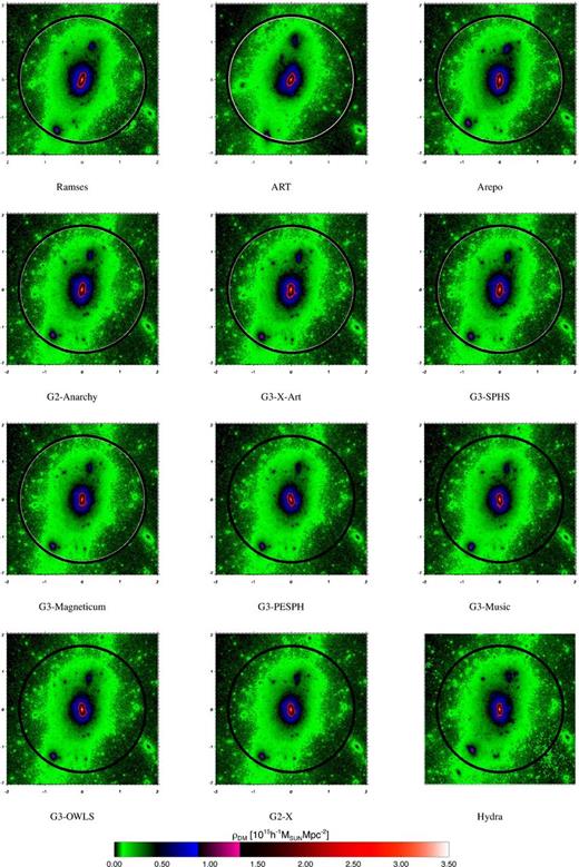
We first completed a dark matter-only simulation, performed using the parameter values given in Table 2. These were chosen independently by each modelling group following their previous experience, so this is in essentially a blind comparison without iteration. A visual comparison of the smoothed density field centred on the cluster at z = 0 is given in Fig. 1. While it is clear that all the methods have followed the formation of the same object (with a significant improvement with respect to fig. 1 of SB99) the precise location of the major subhalo (which is the object located at 7 o'clock with respect to the centre of the cluster in Fig. 1) is not accurately recovered. The variance across this figure illustrates the typical range of outcomes from commonly used cosmological codes. A possible major cause of the discrepancy (for the gadget based codes at least) is the size of the base-level particle mesh, at least for gadget-based codes. Those implementations which employed a base mesh of 2563 did not sufficiently resolve the interface region between this low-resolution mesh and the higher resolution region placed over the cluster: g3-magneticum, g3-pesph and g2-x – the gadget codes which adopted a base mesh of 2563 – show the major subhalo positioned closer to |$R_{200}^{{\rm crit}}$| (the subhalo centre is located at ∼0.9|$R_{200}^{{\rm crit}}$| from the cluster centre) with respect to the codes with a higher base mesh (∼0.75|$R_{200}^{{\rm crit}}$| from the cluster centre). In order to test this effect, we repeated the g3-music run changing only the base-level mesh from 5123 to 2563 and keeping all the other parameters unaltered; as expected, we found that the major subhalo had sensibly moved closer to the virial ratio of the cluster with respect to the original run.
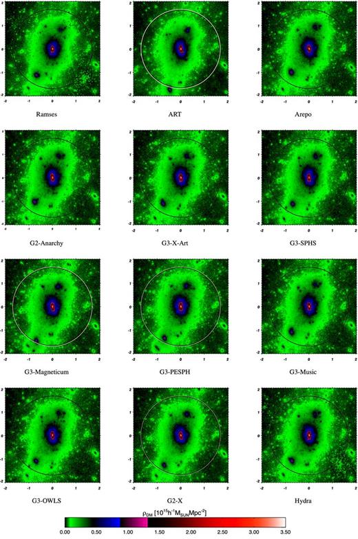
Projected density of the dark matter halo at z = 0 for each simulation as indicated. The box is 2 h−1 Mpc on a side. The white circle indicates |$M_{200}^{{\rm crit}}$| for the halo, the black circle shows the same but for the g3-music simulation.
Improving the resolution of the base-level mesh to 5123 alleviates therefore this problem and aligns the dark matter component well. We illustrate this in Appendix A by reproducing Fig. 1 with all the base-level meshes set to 5123. For the non-radiative comparison described in the next section, we aligned all the codes to a common value of the size of the base level (5123).
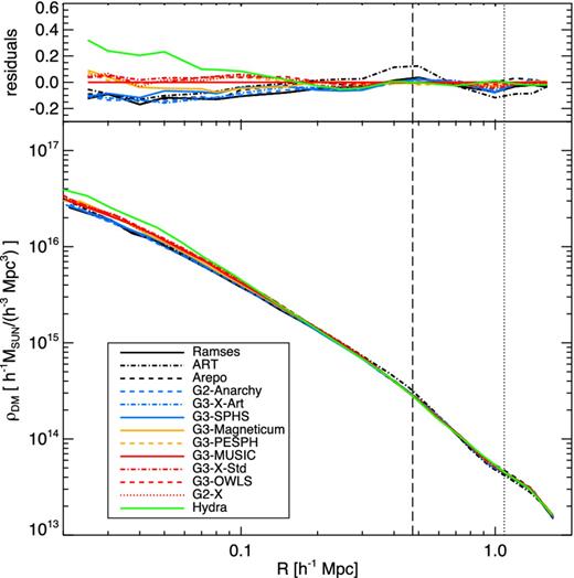
Fig. 2 displays the radially averaged projected dark matter density profiles for the 12 different non-aligned dark matter-only runs, including also the residuals relative to the density profile of the reference g3-music simulation. All the simulations lie well within 10 per cent of each other at all radii with the hydra simulation being indistinguishable from the gadget runs.
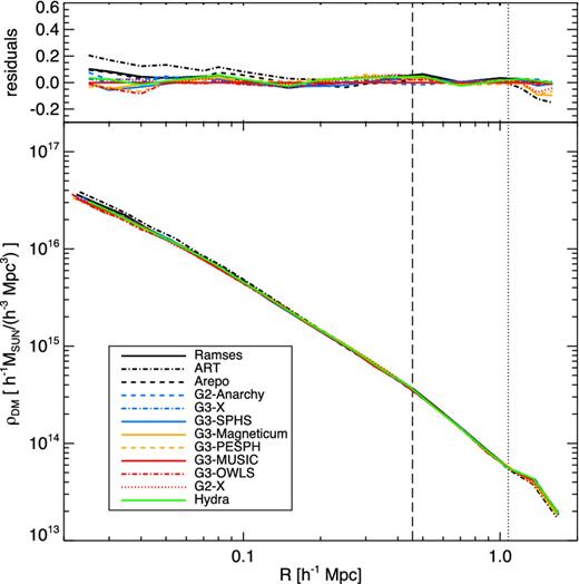
Radial density profiles for the dark matter-only simulations at z = 0 (bottom panel) and the difference between the radial density profiles of each dark matter-only simulation at z = 0 and the reference g3-music density profile (top panel). The vertical dashed line corresponds to R2500 and the vertical dotted line to R500 in the reference g3-music simulation. The radial profiles finish at R200.
The subhalo mass function at z = 0 (Fig. 3) is recovered with only small differences between the models (the differences are always below 20 per cent at all masses). Subhaloes were identified using ahf (Gill, Knebe & Gibson 2004; Knollmann & Knebe 2009; freely available from http://popia.ft.uam.es/AHF). The number of subhaloes is essentially identical except for tiny mass differences which are driven by the small divergences in radial location that were identified above. These code-to-code variations lead to differences in the mass associated with each subhalo as the threshold that defines where a subhalo is separated from the background halo varies. As expected, subhaloes closer to the centre of the main halo than the equivalent subhalo in one of the other models have a lower recovered mass.
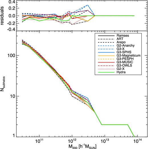
Subhalo mass function for the dark matter-only simulations at z = 0 (bottom panel) and difference between the subhalo mass function of each dark matter-only simulation at z = 0 and the reference g3-music subhalo count (top panel). The lines all overlay each other at M200 > × 1012 h−1 M⊙.
Comparison of the dark matter distribution and of its radial density profile at z = 1 yields results similar to those described above. We conclude that the typical range of chosen parameters for cosmological simulation codes found in the literature introduces a variation of around 10 per cent in the density profile of collapsed objects. This scatter can be reduced to less than 5 per cent by aligning the numerical accuracy of our calculations (see Fig. A1 in Appendix A). Although this is not essential for many applications, we choose to do this in the remainder of this paper so that the underlying dark matter framework agrees closely, allowing us to focus on differences resulting from the various hydrodynamical schemes. Given these concerns we adopt for the non-radiative runs a common set of parameters, including a base-level mesh fixed to 5123 (the full set of aligned parameters is listed in Table A1).
NON-RADIATIVE RUN COMPARISON
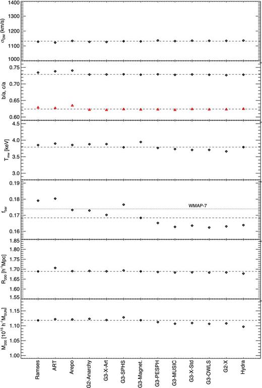
Global properties of the cluster calculated by the different codes. All quantities are computed within |$R_{200}^{{\rm crit}}$|. From top panel to bottom panel: (1) the one-dimensional velocity dispersion of the dark matter; (2) the axial ratio (b/a in black, c/a in red); (3) the mass-weighted temperature; (4) the gas fraction (the dotted line represents the value of the cosmic ratio from WMAP7 (Komatsu et al. 2011); (5) the radius and (6) the total cluster mass. The dashed lines represent the median value for each one of the plotted quantities.
Thumbnail images of the gas density distribution for each of the methods at z = 0 are given in Fig. 5. We see a dramatic variation in the central concentration of the gas, with some methods having significantly larger extended nuclear gas regions.
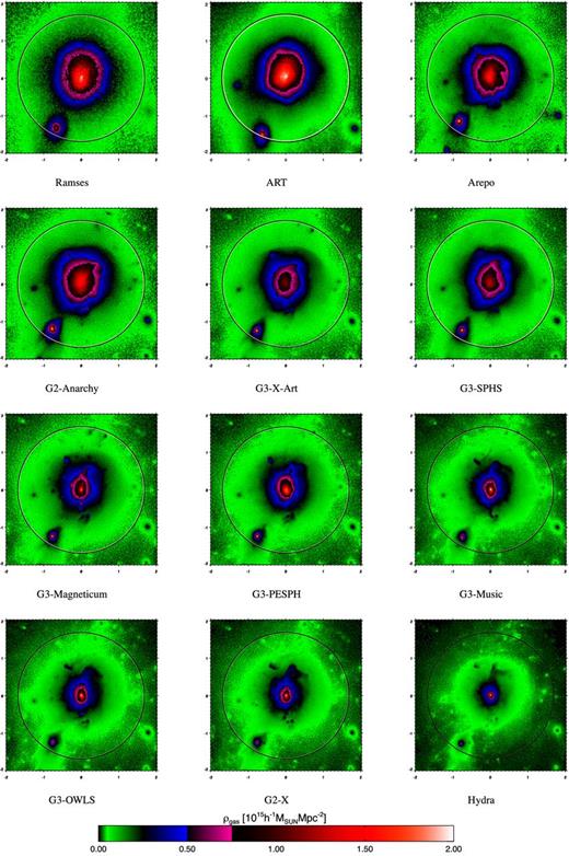
Projected density of the gas halo at z = 0 for each simulation as indicated. The box is 2 h−1 Mpc on a side. The white circle indicates |$M_{200}^{{\rm crit}}$| for the halo, the black circle shows the same but for the g3-music simulation.
This trend is born out by the radial gas density profiles given in Fig. 6. We see that the radial gas density contains a significant core for ramses, art and arepo when compared to the classic SPH schemes employed by some SPH codes such as hydra and g2-x. SPH codes that implement artificial diffusion can produce results that are close to those of ramses and arepo. In between these two extremes the various SPH implementations can produce a range of core sizes in the radial gas density profile.
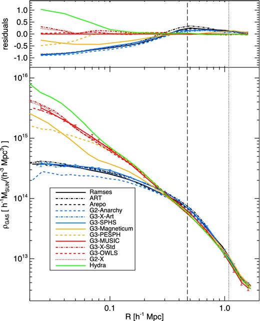
Radial gas density profiles at z = 0 for each simulation as indicated (bottom panel) and difference in radial gas density profiles at z = 0 between each simulation and the reference g3-music simulation. The vertical dashed line corresponds to R2500 and the dotted line to R500 of the reference g3-music values. The error bars on g3-sphs (black) and g3-music (red) are calculated from the scatter between snapshots averaged over the final 0.27 Gyr. The data are cut-off when the radius goes below the softening scale of the code at the inside and at R200 at the outside.
Similarly to all subsequent radial plots the differences in the gas density compared to the fiducial g3-music simulation are shown in the top panel of Fig. 6. At z = 0 the lowest central densities are an order of magnitude lower than in the g3-music simulation while the highest central densities are around two to three times larger, i.e. the variation in the central gas density across our runs is well over an order of magnitude. The scatter becomes more moderate when considering the outer region of the cluster, not exceeding 20 per cent at radii larger than |$R_{2500}^{{\rm crit}}$|.
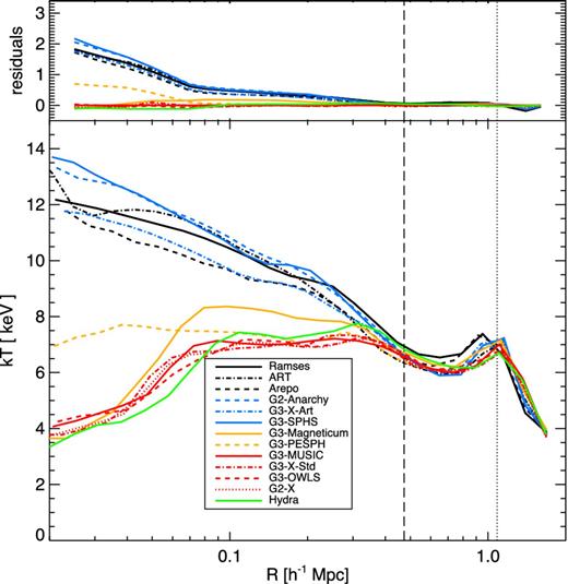
Radial temperature profile at z = 0 for each simulation as indicated and difference between each simulation and the reference g3-music simulation. The vertical dashed line corresponds to R2500 and the vertical dotted line to R500 of the reference g3-music values. The lines terminate at R200 for each model.
At radii larger than |$R_{2500}^{\rm crit}$| the scatter is significantly more moderate, and the residuals appear to be a factor of 2 smaller than in fig. 17 of SB99 in the same cluster regions.
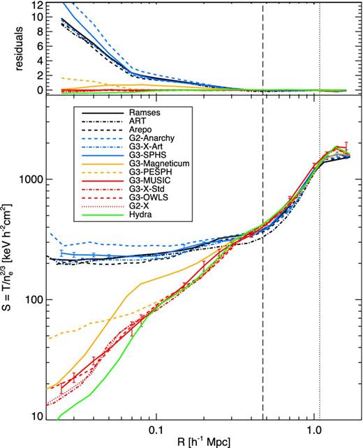
Radial entropy profile at z = 0 (bottom panel) for each simulation as indicated and difference between each simulation and the reference g3-music simulation (top panel). The dashed line corresponds to R2500 and the dotted line to R500 of the reference g3-music values. The error bars on g3-sphs (blue) and g3-music (red) are calculated from the scatter between snapshots averaged over the last 0.27 Gyr.
Other quantities in the non-radiative simulations
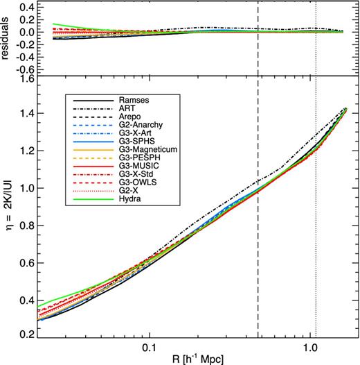
The ratio of kinetic to thermal energy in the gas, η, measured radially at z = 0 for each simulation as indicated (bottom) and difference between each simulation and the reference g3-music simulation (top). The dashed line corresponds to R2500 and the dotted line to R500 of the reference g3-music values.
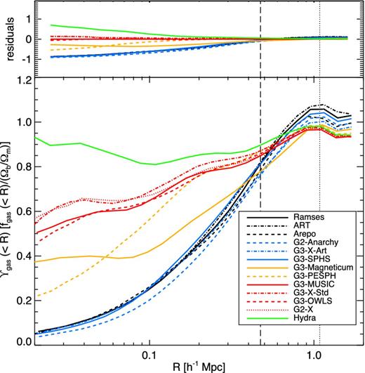
Radial gas fraction at z = 0 relative to the cosmic value for each simulation as indicated (bottom) and difference between each simulation and the reference g3-music simulation (top). The dashed vertical line corresponds to R2500 and dotted vertical line to R500 of the reference g3-music values.
We can combine our measurements of the gas density and temperature to produce Fig. 11, the gas pressure profiles and Fig. 12, the X-ray emission profiles. We define the pressure as P = ρgasT and we normalize the profiles to the value of P500 (the value of the pressure as calculated at |$R_{500}^{\rm crit}$|) in order to be consistent with the definition of universal pressure profile introduced by Arnaud et al. (2010).
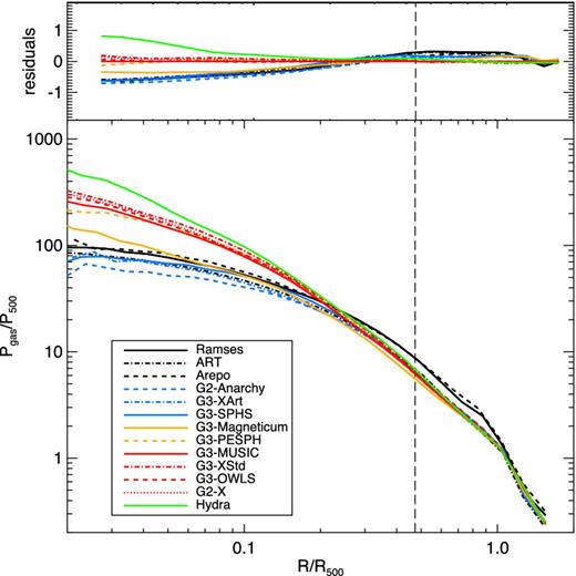
Radial gas pressure at z = 0 measured in each simulation as indicated (bottom panel) and difference between each simulation and the reference g3-music simulation (top panel). The pressure, as well as the radius, has been normalized to the corresponding value at R500 for each code. The dashed vertical line corresponds to R2500 of the reference g3-music value.

Radial X-ray luminosity profiles at z = 0 for each simulation as indicated (bottom panel) and difference between each simulation and the reference g3-music simulation (top panel). The dashed vertical line corresponds to R2500 and the dotted vertical line to R500 of the reference g3-music values.
The X-ray luminosity profile is defined as |$4\pi R^3\mathcal {L}_{\rm X}$| and we approximate the X-ray luminosity density as |$\mathcal {L}_{\rm X} \propto \rho _{{\rm gas}}^2T^{1/2}$|. The variation in the gas density and temperature produce very different pressure and X-ray emission profiles.
As expected, the pressure profiles continue to rise all the way into the centre for all codes (as the central gas is close to hydrostatic equilibrium in all cases). Because of the very high central density, the central X-ray emission for hydra is over two orders of magnitude higher than that found by the grid-based codes and some modern SPH methods which form extended cores.
CONVERGENCE AND SCATTER BETWEEN SIMULATIONS
Dark matter-only runs
We began with an essentially blinded simulation of the same dark matter cluster. By doing this we discovered that the major cause of the discrepancy (for the gadget-based codes at least) between the methods is the size of the base-level particle mesh. Between this and the refined region that covers the cluster there is a resolution jump, typically to an effective resolution of at least 20483. A base mesh of 2563 is not sufficient to resolve the interface region between the low-resolution region (i.e. the base level) and the high-resolution region (i.e. the refined level) placed over the cluster; we found that a base-level of at least 5123 is required to ensure that the dark matter component is well aligned across the different codes. We then resimulated the cluster with an agreed set of matching parameters. For the N-body only simulations we find excellent agreement between the density profiles of the main halo and the statistics of their subhaloes (Figs 2 and 3), once the input parameters of the various runs are matched (see Appendix A). The numerous implementations of gadget, ramses and hydra agree remarkably well, although the gadget agreement is perhaps not surprising given that the gravity solver is in each case built on the same foundation.
Variation amongst classic SPH methods
Despite the excellent agreement between the dark matter-only runs, the classic SPH simulations also show scatter in their central gas density, temperature and entropy that is significantly larger than the theoretical error on each (as calculated from the scatter between snapshots averaged over the final 0.27 Gyr; see the error bars marked on the plots shown in Figs 6 and 8). This is likely because in classic SPH entropy mixing is extremely low and so the final entropy profile forms a historical record reflecting the result of all the mergers that formed the cluster. The resultant radial profile is well sorted in entropy as low entropy material sinks and high entropy material rises. Small differences between the codes in their ability to resolve the entropy jumps due to accretion shocks are therefore amplified by the final time (Power et al. 2014). Nevertheless, a similar scatter is observed also for the gas density profiles of modern SPH codes, suggesting that the lack of mixing may not be the only cause of the discrepancies. We recall that the behaviour of low entropy particles in the real ICM, which depends on how the different phases mix, is largely unknown.
Variation between modern SPH methods and grid-based schemes
Of considerable interest are the differences between the modern SPH flavours (g3-x-art; g3-sphs; g2-anarchy; g3-pesph; g3-magneticum) and the grid-based schemes. There is excellent agreement between the dark matter distributions across the runs, which allows us to isolate the effect of the hydrodynamics solver (Fig. A2). This agreement for the dark matter is somewhat overemphasized by the plots because all the gadget methods and arepo use the same underlying gravity solver. However, ramses and hydra are not related to the gadget family and still look remarkably similar for the dark matter (see Fig. A1 for example).
For the radial gas density profiles shown in Fig. 6, ramses, arepo and g3-x-art are in excellent agreement with one another and g3-sphs and art only show some moderate discrepancies, while g2-anarchy seems to be an outlier. In Fig. 7 the temperature profiles for arepo and g3-x-art are very closely matched but look to have an offset from g3-sphs and g2-anarchy, which are very close to one other. ramses produces a result that is intermediate between these two pairs. art produces a temperature lower than the other two grid-based codes outside of the cluster centre. In Fig. 8 the radial entropy profiles of g3-sphs, g3-x-art and ramses are again very close to one another while g2-anarchy is somewhat higher and arepo somewhat lower. art show a lower entropy in the region around R500. The origin of these differences is yet to be explained, although we note that it cannot be attributed to different merger phases and must result from the hydrodynamics solver. In the case of g2-anarchy a possible cause of discrepancy may be the choice of the kernel (using a C4 kernel with 200 neighbours gives slightly different values for the central entropy). Power et al. (2014) showed that at the resolution of the simulations in this paper, g3-sphs is numerically converged. It would be interesting to see if the remaining differences between g3-sphs, g3-x-art, arepo, ramses, art and g2-anarchy remain with increasing resolution. We defer such a resolution study to future work, whose intent will be to narrow down these numerical uncertainties.
The arepo simulations use the total energy as a conserved quantity in the Godunov scheme, which is the usual choice in finite volume codes and the same choice as that used in the most recent arepo studies (as e.g. in Vogelsberger et al. 2014). As discussed in Springel (2010), using an entropy-energy formalism results in smaller entropy cores and higher central gas densities somewhat closer to classic SPH results (similar results are also shown by gizmo; Hopkins 2015). Following most recent arepo studies, we have not employed the latter method here due to concerns regarding the artificial suppression of weak shocks and the potentially less accurate energy conservation.
Finally, we note that the results of g3-pesph are very different from those of the other modern SPH flavours (with the exception of g3-magneticum), and are more similar to those of classic SPH simulations. A key difference is that this version of g3-pesph does not include any explicit conductivity or mixing, while all the other modern variants do. Hu et al. (2014) showed that g3-pesph performs much better than previous versions of SPH for surface instabilities by greatly mitigating surface tension problems, but in areas of very strong shocks (M ∼ 1000) adding artificial conduction provides a better match to analytic solutions. Insights into the behaviour of g3-pesph may be gained by considering the SPH method presented in Read et al. (2010), and the earlier multiphase method by Ritchie & Thomas (2001). As pointed out by Read & Hayfield (2012), the Richie & Thomas method only works well for relatively small entropy contrasts between different fluid phases. As the entropy contrast becomes very large, the admixture of low and high entropy particles within the smoothing kernel creates large pressure fluctuations that prevent mixing, as in classic SPH. This was recognized also by Ritchie & Thomas (2001) who proposed scaling the neighbour number with the entropy contrast to combat this. However, this rapidly becomes prohibitively expensive in real-world applications, which led Read & Hayfield (2012) to abandon such methods in favour of dissipation switching, as proposed by Price (2008); such switching is common to g3-x-art, g3-sphs and g2-anarchy and helps to explain their similarity. The discrepancy between g3-pesph and the other modern SPH flavours may also reflect the treatment of artificial viscosity. They all adopt the artificial viscosity model suggested by Cullen & Dehnen (2010) which can produce larger entropy gains in shocks while the authors of g3-pesph do not use this because it also seems to add substantial entropy into very diffuse intergalactic gas that may be spurious (Katz, private communication). In short, it is unclear how much artificial conductivity and/or mixing is appropriate in SPH, or even whether the mesh-based codes are providing the correct solution that all SPH codes should be trying to emulate. Nonetheless, consistency with mesh codes appears to require modern SPH using conduction, mixing and a higher order dissipation switch.
SUMMARY AND CONCLUSIONS
We have investigated the performance of 13 modern astrophysical simulation codes – ramses, art, arepo, hydra and nine versions of gadget with different SPH implementations – by carrying out cosmological zoom simulations of a single massive galaxy cluster. Our goal was to assess the consistency of the different codes in reproducing the spatial and thermodynamical structure of the dark matter and non-radiative gas in a galaxy cluster.
As our initial step, we ran dark matter-only versions of the simulations with each simulation team using their preferred set of numerical parameters (e.g. time step accuracy, gravitational softening, dimension of the particle mesh), and examined the spherically averaged mass density profile and the spatial distribution of substructures. We found good consistency between the density profiles recovered by the codes at approximately the 10 per cent level, while there were small variations in the positions of substructures. When these simulations were re-run with an agreed common set of numerical parameters, we found that these small variations could be suppressed (essentially entirely, in the case of the gadget codes).
By adopting this common parameter set, we were able to isolate those differences between the results of the hydrodynamical simulations that arise only from the choice of hydrodynamical solver, rather than from the complex interplay of the hydrodynamical and gravity solvers. As expected from the wide range of hydrodynamical implementations covered we found that the resulting gas density profiles varied substantially amongst the codes. Our key findings can be summarized as follows.
Some codes, essentially the oldest, with classic SPH implementations, exhibit continually falling inner entropy profiles, without any evidence of an entropy core. This is because these codes, particularly hydra, were carefully designed to be entropy conserving with very low levels of mixing. This lack of mixing preserves low-entropy gas particles at the centres of all objects, including subhaloes, which survive until late times. As the cluster relaxes, these particles sink to the centre of the radial density profile, decreasing the central entropy.
In contrast, the grid-based codes ramses, art and arepo produce extended cores with a large constant entropy core. In these mesh-based codes mixing of entropy arises as a consequence of the numerical diffusion associated with the Riemann solver: they naturally mix entropy between gas elements, essentially eliminating the very low entropy material.
Modern SPH codes such as g2-anarchy, g3-sphs and g3-x-art, which have dissipative switches and new kernels, can bridge the gap between the classic SPH codes and grid-based codes, producing entropy cores that are indistinguishable from those of the grid-based schemes.
Our results confirm that the discrepancies between grid-based codes and SPH codes in describing the radial entropy profile of simulated clusters, identified by the Santa Barbara Cluster Comparison Project presented in SB99, can be overcome by modern SPH codes. Importantly, all the codes employed in this work succeed in recovering the global properties and most of the radial profiles of a simulated large galaxy cluster with much greater accuracy and significantly smaller scatter than those presented in SB99; this highlights the enormous strides in the development of astrophysical hydrodynamical simulation codes over the last decade.
This work constitutes the first in a series of papers in which we examine in detail the predictions of modern astrophysical hydrodynamical simulation codes. The next paper in this series will focus on simulations of the same galaxy cluster, now modelled with a variety of galaxy formation processes including cooling, star formation, supernovae and feedback from AGN. This will allow us to establish how radiative processes affect the entropy cores of simulated clusters. Subsequent papers will look at the recovery of cluster properties such as X-ray temperature and Sunyaev–Zel'dovich profiles, gravitational lensing and cluster outskirts and hydrostatic-mass bias; all of which will add to our understanding of how consistently the results of different codes can inform our understanding of galaxy cluster properties.
The authors would like to express special thanks to the Instituto de Fisica Teorica (IFT-UAM/CSIC in Madrid) for its hospitality and support, via the Centro de Excelencia Severo Ochoa Program under Grant No. SEV-2012-0249, during the three-week workshop ‘nIFTy Cosmology’ where this work developed. We further acknowledge the financial support of the University of Western 2014 Australia Research Collaboration Award for ‘Fast Approximate Synthetic Universes for the SKA’, the ARC Centre of Excellence for All Sky Astrophysics (CAASTRO) grant number CE110001020, and the two ARC Discovery Projects DP130100117 and DP140100198. We also recognize support from the Universidad Autonoma de Madrid (UAM) for the workshop infrastructure.
AK is supported by the Ministerio de Economía y Competitividad (MINECO) in Spain through grant AYA2012-31101 as well as the Consolider-Ingenio 2010 Programme of the Spanish Ministerio de Ciencia e Innovación (MICINN) under grant MultiDark CSD2009-00064. He also acknowledges support from the Australian Research Council (ARC) grants DP130100117 and DP140100198. He further thanks France Gall for le coeur qui jazze. CP acknowledges support of the Australian Research Council (ARC) through Future Fellowship FT130100041 and Discovery Project DP140100198. WC and CP acknowledge support of ARC DP130100117. EP acknowledges support by the ERC grant ‘The Emergence of Structure during the epoch of Reionization’. STK acknowledges support from STFC through grant ST/L000768/1. RJT acknowledges support via a Discovery Grant from NSERC and the Canada Research Chairs program. Simulations were run on the CFI-NSRIT funded Saint Mary's Computational Astrophysics Laboratory. SB and GM acknowledge support from the PRIN-MIUR 2012 Grant ‘The Evolution of Cosmic Baryons’ funded by the Italian Minister of University and Research, by the PRIN-INAF 2012 Grant ‘Multi-scale Simulations of Cosmic Structures’, by the INFN INDARK Grant and by the ‘Consorzio per la Fisica di Trieste’. IGM acknowledges support from a STFC Advanced Fellowship. PJE is supported by the SSimPL program and the Sydney Institute for Astronomy (SIfA), DP130100117. JIR acknowledges support from SNF grant PP00P2 128540/1. CDV acknowledges financial support from the Spanish Ministry of Economy and Competitiveness (MINECO) through the 2011 Severo Ochoa Program MINECO SEV-2011-0187 and the AYA2013-46886-P grant. AMB is supported by the DFG Research Unit 1254 ‘Magnetisation of Interstellar and Intergalactic Media’ and by the DFG Cluster of Excellence ‘Origin and Structure of the Universe’. RDAN acknowledges the support received from the Jim Buckee Fellowship. The arepo simulations were performed with resources awarded through STFCs DiRAC initiative. The authors thank Volger Springel for helpful discussions and for making arepo and the original gadget version available for this project. G3-PESPH simulations were carried out using resources at the Center for High Performance Computing in Cape Town, South Africa.
The authors contributed to this paper in the following ways: FS, GY, FRP, AK, CP, STK and WC formed the core team that organized and analysed the data, made the plots and wrote the paper. AK, GY and FRP organized the nIFTy workshop at which this program was completed. GY supplied the initial conditions. PJE assisted with the analysis. All the other authors, as listed in Section 2 performed the simulations using their codes. All authors had the opportunity to proof read and comment on the paper.
The simulation used for this paper has been run on Marenostrum supercomputer and is publicly available at the MUSIC website.4
This research has made use of NASA's Astrophysics Data System (ADS) and the arXiv preprint server.
Specifically, it is cluster 19 of MUSIC-2 data set; all the initial conditions of MUSIC clusters are available at http://music.ft.uam.es
REFERENCES
APPENDIX A: DARK MATTER ALIGNMENT
In order to perform a clean comparison of the various gas physics implementations we carefully aligned the underlying gravitational framework for each model. While Fig. 1 illustrates the range of outcomes that result in the dark matter-only runs from a blind comparison using individual parameter choices, we can choose a common parameter set for those quantities that control the accuracy of the gravitational forces. For instance, for gadget, Table A1 gives the parameter choices made independently by each group. The final row lists the common parameter set adopted for the non-radiative comparison. The improvement in the alignment between the different methods is shown in Fig. A1, which displays the dark matter radial profiles of the dark matter-only simulations re-run using the common parameters listed in Table A1. After fixing the base-level mesh to the common value of 5123, the scatter in the profiles among different codes is below 10 per cent. We tested that increasing the resolution of the base-level mesh further to 10243 did not result in further movement of this substructure. The largest reduction of scatter is seen in the outskirts, where the location of most massive subhalo around the 7 o'clock position is well matched just inside R200. Despite this improvement, the ART profile shows deviation of order 10 per cent due to the positional offset of another massive subhalo around the 12 o'clock position. As we advance the ART run by ∼20 per cent of the dynamical time of the cluster at R200, we are able to better match the position of this subhalo, indicating that this is due to timing offset. Further investigation is needed, and we plan to do so in our follow-up work using multiple haloes with varying dynamical states.
Radial density profiles for the dark matter-only simulations with aligned parameters at z = 0 (bottom panel) and difference between the radial density profiles of dark matter-only simulation at z = 0 and the reference g3-music density profile (top panel). The vertical dashed line corresponds to R2500 and the vertical dotted line to R500 of the reference g3-music values.
Numerical parameters used for the arepo and gadget runs: accuracy of the time step (ETIA), time step displacement factor (MRDF), minimum (MINT) and maximum (MAXT) time step, tolerance on the force accuracy (ETFA), accuracy of the tree algorithm (ETT), Courant factor (CFAC), double precision (DP, DF) and the number of FFT cells along each side of the box (NFFT).
| Code name | ETIA | MRDF | MINT | MAXT | ETFA | ETT | CFAC | DP | DF | NFFT |
|---|---|---|---|---|---|---|---|---|---|---|
| arepo | 0.025 | 0.125 | 0 | 0.01 | 0.0025 | 0.6 | 0.3 | Y | Y | 512 |
| g2-anarchy | 0.01 | 0.125 | 0.0 | 0.01 | 0.025 | 0.3 | 0.3 | Y | Y | 512 |
| g3-x-art | 0.01 | 0.5 | 0 | 0.01 | 0.01 | 0.45 | 0.15 | N | N | 512 |
| g3-sphs | 0.03 | 0.5 | 0 | 0.02 | 0.005 | 0.5 | 0.4 | N | N | 1024 |
| g3-magneticum | 0.05 | 0.25 | 0 | 0.05 | 0.005 | 0.45 | 0.15 | Y | Y | 256 |
| g3-pesph | 0.05 | 0.25 | 10−7 | 0.05 | 0.005 | 0.4 | 0.15 | Y | Y | 256 |
| g3-music | 0.01 | 0.5 | 0 | 0.01 | 0.01 | 0.4 | 0.15 | Y | Y | 512 |
| g3-owls | 0.025 | 0.25 | 10−10 | 0.025 | 0.005 | 0.6 | 0.15 | Y | N | 1024 |
| g2-x | 0.02 | 0.25 | 10−7 | 0.025 | 0.0025 | 0.3 | 0.15 | Y | Y | 256 |
| Common parameter set | 0.01 | 0.125 | 0.0 | 0.01 | 0.025 | 0.3 | 0.15 | Y | Y | 512 |
For this common choice the gravitational evolution of all the simulations is also essentially indistinguishable in the non-radiative case, as illustrated by Fig. A2, which gives visual images of the dark matter distribution in the non-radiative runs. Fig. A3 shows the radial density distribution of the dark matter in the non-radiative case, and the difference relative to the g3-music simulation. For hydra, the central gas density is so high that it steepens the central dark matter distribution relative to the other codes. As a consequence of adding the gas, the scatter in the radial dark matter density profile is higher than that seen in the dark matter-only runs. There is also a marked split between those codes that produce a core in the radial gas distribution and those that do not. This is in the sense expected and demonstrates the expected back-reaction in the dark matter potential. As in the case of dark matter-only aligned simulations, the difference in the profiles of art is due to mismatch of the main subhalo in the 12 o'clock position caused by timing offset, which we will investigate in detail in another upcoming paper.
Projected density of the dark matter halo in the non-radiative simulations at z = 0 for each method as indicated. The box is 2 h−1 Mpc on a side. The white circle indicates |$M^{200}_{{\rm crit}}$| for the halo, the black circle the same but for the g3-music simulation.
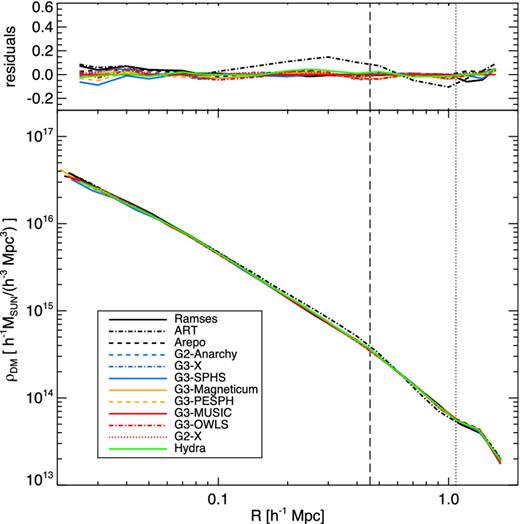
Radial dark matter density profiles for the non-radiative simulations at z = 0 (bottom panel) and difference between the radial density profiles of each non-radiative simulation at z = 0 and the reference g3-music density profile (top panel). The vertical dashed line corresponds to R2500 and the vertical dotted line to R500 of the reference g3-music values.
