


Abstract
The Sun is the only star whose surface can be directly resolved at high resolution, and therefore constitutes an excellent test case to explore the physical origin of stellar radial-velocity (RV) variability. We present HARPS observations of sunlight scattered off the bright asteroid 4/Vesta, from which we deduced the Sun's activity-driven RV variations. In parallel, the Helioseismic and Magnetic Imager instrument on board the Solar Dynamics Observatory provided us with simultaneous high spatial resolution magnetograms, Dopplergrams and continuum images of the Sun in the Fe i 6173 Å line. We determine the RV modulation arising from the suppression of granular blueshift in magnetized regions and the flux imbalance induced by dark spots and bright faculae. The rms velocity amplitudes of these contributions are 2.40 and 0.41 m s−1, respectively, which confirms that the inhibition of convection is the dominant source of activity-induced RV variations at play, in accordance with previous studies. We find the Doppler imbalances of spot and plage regions to be only weakly anticorrelated. Light curves can thus only give incomplete predictions of convective blueshift suppression. We must instead seek proxies that track the plage coverage on the visible stellar hemisphere directly. The chromospheric flux index |$R^{\prime }_{HK}$| derived from the HARPS spectra performs poorly in this respect, possibly because of the differences in limb brightening/darkening in the chromosphere and photosphere. We also find that the activity-driven RV variations of the Sun are strongly correlated with its full-disc magnetic flux density, which may become a useful proxy for activity-related RV noise.
INTRODUCTION
The surface of a star is constantly bustling with magnetic activity. Starspots and faculae/plage1 inhibit convective motions taking place at the stellar surface, thus suppressing part of the blueshift naturally resulting from granulation. In addition, dark starspots (and bright faculae, to a lesser extent) coming in and out of view as the star rotates induce an imbalance between the redshifted and blueshifted halves of the star, which translates into a radial-velocity (RV) variation. Stellar activity, through the perturbation of photospheric convection, induces RV variations on much longer time-scales of the order of years, in tune with their magnetic cycles (e.g. see Santos et al. 2010; Dumusque et al. 2011; Díaz et al. 2016).
Short-term activity-induced RV variations are quasi-periodic: they are modulated by the star's rotation and change as active regions (starspots and faculae) emerge, evolve and disappear. The amplitude of these variations is 1–2 m s−1 in ‘quiet’ stars (Isaacson & Fischer 2010), but they are often larger than this and can mimic or conceal the Doppler signatures of orbiting planets. This has resulted in several false detections (see Queloz et al. 2001; Bonfils et al. 2007; Huélamo et al. 2008; Boisse et al. 2009, 2011; Gregory 2011; Haywood et al. 2014; Robertson et al. 2014; Santos et al. 2014 and many others).
Understanding the RV signatures of stellar activity, especially those at the stellar rotation time-scale, is essential to develop the next generation of more sophisticated activity models and further improve our ability to detect and characterize (super-)Earths and even small Neptunes in orbits of a few days to weeks. In particular, identifying informative and reliable proxies for the activity-driven RV variations is crucial. Desort et al. (2007) found that the traditional spectroscopic indicators [the bisector span (BIS) and full width at half-maximum (FWHM) of the cross-correlation profile] and photometric variations do not give enough information for slowly rotating, Sun-like stars (low v sin i) to disentangle stellar activity signatures from the orbits of super-Earth-mass planets.
The Sun is a unique test case as it is the only star whose surface can be resolved at high resolution, therefore allowing us to investigate directly the impact of magnetic features on RV observations. Early attempts to measure the RV of the integrated solar disc did not provide quantitative results about the individual activity features responsible for RV variability. Jiménez et al. (1986) measured integrated sunlight using a resonant scattering spectrometer and found that the presence of magnetically active regions on the solar disc led to variations of up to 15 m s−1. They also measured the disc-integrated magnetic flux but did not find any significant correlation with RV at the time due to insufficient precision. At about the same time, Deming et al. (1987) obtained spectra of integrated sunlight with an uncertainty level below 5 m s−1, enabling them to see the RV signature of supergranulation. The trend they observed over the 2-yr period of their observations was consistent with suppression of convective blueshift from active regions on the solar surface. A few years later, Deming & Plymate (1994) confirmed the findings of both Jiménez et al. (1986) and Deming et al. (1987), only with a greater statistical significance. Not all studies were in agreement with each other; however, McMillan et al. (1993) recorded spectra of sunlight scattered off the Moon over a 5-yr period and found that any variations due to solar activity were smaller than 4 m s−1.
More recently, Molaro & Centurión (2010) obtained HARPS spectra of the large and bright asteroid Ceres to construct a wavelength atlas for the Sun. They found that these spectra of scattered sunlight provided precise disc-integrated solar RVs, and proposed using asteroid spectra to calibrate high-precision spectrographs used for planet hunting, such as HIRES and HARPS (see a recent paper by Lanza et al. 2016).
In parallel, significant discoveries were made towards a precise quantitative understanding of the RV impact of solar surface features. Lagrange, Desort & Meunier (2010) and Meunier, Desort & Lagrange (2010a) used a catalogue of sunspot numbers and sizes and Michelson Doppler Imager/Solar and Heliospheric Observatory (MDI/SOHO) magnetograms to simulate integrated-Sun spectra over a full solar cycle and deduce the impact of sunspots and faculae/plage on RV variations. The work of Meunier et al. (2010a) also relied on the amplitude of convection inhibition derived by Brandt & Solanki (1990), based on spatially resolved magnetogram observations of plage and quiet regions on the Sun (i.e. independently of full-disc RV measurements).
Sunspot umbrae and penumbrae are cooler and therefore darker than the surrounding quiet photosphere, producing a flux deficit at the local rotational velocity. Faculae, which tend to be spatially associated with spot groups, are slightly brighter than the quiet photosphere, producing a spectral flux excess at the local rotational velocity. Spots have large contrasts and small area coverage, while faculae have lower contrasts but cover large areas. We thus expect their rotational Doppler signals to be of opposite signs (due to the opposite sign of their flux) and of roughly similar amplitudes. However, facular emission also occurs independently of spot activity in the more extended solar magnetic network (Chapman et al. 2001), so their contributions do not cancel out completely. Meunier et al. (2010a) found that the residual signal resulting from the rotational Doppler imbalance of both sunspots and faculae is comparable to that of the sunspots on their own. Lagrange et al. (2010) estimated the rotational perturbation due to sunspot flux deficit to be of the order of 1 m s−1. In a complementary study, Meunier et al. (2010a) also investigated the effect of sunspots and faculae on the suppression of convective blueshift by magnetic regions. Sunspots occupy a much smaller area than faculae, and as they are dark, they contribute little flux, so their impact on the convective blueshift is negligible. Facular suppression of granular blueshift, however, can lead to variations in RV of up to 8–10 m s−1 (Meunier et al. 2010a). Meunier, Lagrange & Desort (2010b) estimated the disc-integrated solar RV variations expected from the suppression of convective blueshift, directly from MDI/SOHO Dopplergrams and magnetograms (in the 6768 Å Ni i line). Their reconstructed RV variations, over one magnetic cycle, agree with the simulations of Meunier et al. (2010a), establishing the suppression of convective blueshift by magnetic features as the dominant source of activity-induced RV variations. Meunier et al. (2010b) also found that the regions where the convective blueshift is most strongly attenuated correspond to the most magnetically active regions, as was expected.
Following the launch of the Solar Dynamics Observatory (SDO; Pesnell, Thompson & Chamberlin 2012) in 2010, continuous observations of the solar surface brightness, velocity and magnetic fields have become available with image resolution finer than the photospheric granulation pattern. This allows us to probe the RV variations of the Sun in unprecedented detail. In the present paper, we deduce the activity-driven RV variations of the Sun based on HARPS observations of the bright asteroid Vesta (Section 2). In parallel, we use high spatial resolution continuum, Dopplergram and magnetogram images of the Fe i 6173 Å line from the Helioseismic and Magnetic Imager (HMI/SDO; Schou et al. 2012) to model the RV contributions from sunspots (and pores), faculae and granulation via inhibition of granular blueshift and flux blocking (Section 3). This allows us to create a model which we test against the HARPS observations (Section 4). Finally, we discuss the implications of our study for the effectiveness of various proxy indicators for activity-driven RV variations in stars. We show that the disc-averaged magnetic flux could become an excellent proxy for activity-driven RV variations on other stars (Section 5).
HARPS OBSERVATIONS OF SUNLIGHT SCATTERED OFF VESTA
HARPS spectra
The HARPS spectrograph, mounted on the European Southern Observatory 3.6 m telescope at La Silla, was used to observe sunlight scattered from the bright asteroid 4/Vesta (its average magnitude during the run was 7.6). Two to three measurements per night were made with simultaneous Thorium exposures for a total of 98 observations, spread over 37 nights between 2011 September 29 and December 7. The geometric configuration of the Sun and Vesta relative to the observer is illustrated in Fig. 1. At the time of the observations, the Sun was just over three years into its 11-yr magnetic cycle; the SDO data confirm that the Sun showed high levels of activity.

Schematic representation of the Sun, Vesta and Earth configuration during the period of observations (not to scale).
The spectra were reprocessed using the HARPS Data Reduction Software (DRS) pipeline (Baranne et al. 1996; Lovis & Pepe 2007). Instead of applying a conventional barycentric correction, the wavelength scale of the calibrated spectra was adjusted to correct for the Doppler shifts due to the relative motion of the Sun and Vesta, and the relative motion of Vesta and the observer (see Section 2.3).
The FWHM and BIS (as defined in Queloz et al. 2001) and |$\log R^{\prime }_{HK}$| index were also derived by the pipeline. The median, minimum and maximum signal-to-noise ratio of the reprocessed HARPS spectra at central wavelength 556.50 nm are 161.3, 56.3 and 257.0, respectively. Overall, HARPS achieved a precision of 75 ± 25 cm s−1 (see Table A1). The reprocessed HARPS cross-correlation functions and derived RV measurements are available in the Supplementary Files that are available online.
We account for the RV modulation induced by Vesta's rotation in Section 2.4.1, and investigate sources of intra-night RV variations in Section 2.4.2. We selected the SDO images in such a way as to compensate for the different viewing points of Vesta and the SDO spacecraft: Vesta was trailing SDO, as shown in Fig. 1. This is taken into account in Section 2.5.
Solar rest frame
(1) vsv: the velocity of Vesta relative to the Sun at the instant that light received at Vesta was emitted by the Sun;
(2) vve: the velocity of Vesta relative to Earth at the instant that light received by HARPS was emitted at Vesta.
This correction accounts for the RV contribution of all bodies in the Solar system and places the Sun in its rest frame. The values of RVbary,Earth, vsv and vve are given in the Supplementary Files that are available online.
Relativistic Doppler effects
We apply this correction twice:
(1) The light is emitted by the Sun and received at Vesta. In this case, v is the magnitude of the velocity of Vesta with respect to the Sun (decreasing from approximately 19.9 to 19.4 km s−1 over the duration of the HARPS run), and the radial component v cos θo is equal to vsv (defined in Section 2.2, starting at about 1.66 km s−1 and reaching 1.72 km s−1 at opposition near the middle of the run).
(2) Scattered sunlight is emitted from Vesta and received at La Silla. v is the magnitude of the velocity of Vesta with respect to an observer at La Silla (increasing from 20 to 36 km s−1 over the run), and v cos θo is vve (starting at 19.8 km s−1 and reaching 23.3 km s−1 at opposition).
The two wavelength correction factors are then multiplied together in order to compute the total relativistic correction factor to be applied to the pixel wavelengths in the HARPS spectra, from which we derive the correct RVs, shown in Fig. 2(a) (see also column 2 of Table A1). All velocities are measured at the flux-weighted mid-exposure times of observation (MJDmid_UTC).
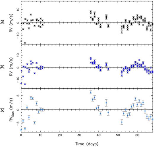
(a) HARPS RV variations in the solar rest frame, corrected for relativistic Doppler effects (but not yet corrected for Vesta's axial rotation). (b) HARPS RV variations of the Sun as a star (after removing the RV contribution of Vesta's axial rotation). (c) Nightly binned HARPS RV variations of the Sun as a star – note the change in scale on the y-axis. The values for each time series are provided in the Supplementary Files that are available online.
The reader may also refer to appendix A of Lanza et al. (2016) for further details on these Doppler corrections. All quantities used to calculate these effects are listed in the Supplementary Files that are available online.
Sources of intra-night RV variations
Vesta's axial rotation
Vesta rotates every 5.34 h (Stephenson 1951), so any significant inhomogeneities in its shape or surface albedo will induce an RV modulation. Vesta's shape is close to a spheroid (Thomas et al. 1997), and Lanza & Molaro (2015) found that the RV modulation expected from shape inhomogeneities should not exceed 0.060 m s−1.
Fig. 2(b) shows the RV observations obtained after subtracting Vesta's rotational signature, with coefficients C and S of equation (7) derived from the global fit of Section 4.1. The night-to-night scatter has been reduced, even though much of it remains in the first block of observations; this is discussed in the following section.
Additional intra-night scatter in first half of HARPS run
The RV variations in the first part of the HARPS run (nights 0 to 11 in Fig. 2) contain some significant scatter, even after accounting for Vesta's rotation. This intra-night scatter does not show in the solar FWHM, BIS or |$\log (R^{\prime }_{HK})$| variations. We investigated the cause of this phenomenon and excluded changes in colour of the asteroid or instrumental effects as a potential source of additional noise. Vesta was very bright (7.6 mag), so we deem the phase and proximity of the Moon unlikely to be responsible for the additional scatter observed.
Solar p-mode oscillations dominate the Sun's power spectrum at a time-scale of about 5 min. Most of the RV oscillations induced by p-mode acoustic waves are therefore averaged out within the 15-min HARPS exposures. Granulation motions result in RV signals of several m s−1, over time-scales ranging from about 15 min to several hours. Taking multiple exposures each night and averaging them together (as plotted in panel (c) of Fig. 2) can help to significantly reduce granulation-induced RV variations.
The remaining variations, of the order of 7–10 m s−1, are modulated by the Sun's rotation and are caused by the presence of magnetic surface markers, such as sunspots and faculae. These variations are the primary focus of this paper, and we model them using SDO/HMI data in Section 3.
Time lag between Vesta and SDO observations
At the time of the observations, the asteroid Vesta was trailing the SDO spacecraft, which orbits the Earth (see Fig. 1). In order to model the solar hemisphere facing Vesta at time t, we used SDO images recorded at t + Δt, where Δt is proportional to the difference in the Carrington longitudes of the Earth/SDO and Vesta at the time of the HARPS observation. These longitudes were retrieved from the JPL Horizons data base. The shortest delay, at the start of the observations, was ∼2.8 d, while at the end of the observations it reached just over 6.5 d (see Table A1). We cannot account for the evolution of the Sun's surface features during this time, and must assume that they remain frozen in this interval. The emergence of sunspots can take place over a few days, but in general large magnetic features (sunspots and networks of faculae) evolve over time-scales of weeks rather than days. Visual inspection of animated sequences of SDO images obtained during the campaign revealed no major flux emergence events on the visible solar hemisphere.
PIXEL STATISTICS FROM SDO/HMI images
The spacecraft's motion and the rotation of the Sun introduce velocity perturbations, which we determine in Sections 3.1 and 3.2, respectively. These two contributions are then subtracted from each Doppler image, thus revealing the Sun's magnetic activity velocity signatures. We compute the RV variations due to the suppression of convective blueshift and the flux blocked by sunspots on the rotating Sun in Sections 3.7.3 and 3.7.2. We show that the Sun's activity-driven RV variations are well reproduced by a scaled sum of these two contributions in Section 4. Finally, we compute the disc-averaged magnetic flux and compare it as an RV proxy against the traditional spectroscopic activity indicators in Section 5.
Spacecraft motion
Solar rotation
Solar differential rotation profile parameters from Snodgrass & Ulrich (1990).
| Parameter | Value (deg d−1) |
|---|---|
| α1 | 14.713 |
| α2 | − 2.396 |
| α3 | − 1.787 |
| Parameter | Value (deg d−1) |
|---|---|
| α1 | 14.713 |
| α2 | − 2.396 |
| α3 | − 1.787 |
Solar differential rotation profile parameters from Snodgrass & Ulrich (1990).
| Parameter | Value (deg d−1) |
|---|---|
| α1 | 14.713 |
| α2 | − 2.396 |
| α3 | − 1.787 |
| Parameter | Value (deg d−1) |
|---|---|
| α1 | 14.713 |
| α2 | − 2.396 |
| α3 | − 1.787 |
Flattened continuum intensity
Unsigned magnetic field strength
The noise level in HMI magnetograms is a function of μ (Yeo, Solanki & Krivova 2013). It is lowest for pixels in the centre of the CCD, where it is close to 5 G, and increases towards the edges and reaches 8 G at the solar limb. For our analysis, we assume that the noise level is constant throughout the image with a conservative value |$\sigma _{B_{{\rm obs}, ij}}$| = 8 G, in agreement with the results of Yeo et al. (2013). We therefore set Bobs,ij and Br,ij to 0 for all pixels with a line-of-sight magnetic field measurement (Bobs,ij) below this value.
Identifying quiet-Sun regions, faculae and sunspots
As is routinely done in solar work, we do not consider pixels that are very close to the limb (μij < 0.1), as the limb-darkening model becomes unreliable on the very edge of the Sun. This affects about 1 per cent of the pixels of the solar disc.
The first three panels of Fig. 3 show an SDO/HMI flattened intensitygram, line-of-sight Dopplergram and unsigned radial magnetogram for a set of images taken on 2011 November 10, after removing the contributions from spacecraft motion and solar rotation. We identify quiet-Sun regions, faculae and sunspots by applying magnetic and intensity thresholds.
- Magnetic threshold: the distribution of pixel unsigned observed magnetic field strength as a function of pixel flattened intensity is shown in Fig. 4. In the top histogram and main panel, we see that the distribution of magnetic field strength falls off sharply with increasing field strength. The vast majority of pixels are clustered close to the noise level: these pixels are part of the quiet-Sun surface. Note that the fragmented distribution of pixels with magnetic field strength less than a few gauss arises from the numerical precision in the SDO/HMI images. This is not an issue in our analysis, however, as these pixels are well below the magnetic noise threshold and we set their field value to zero. We separate active regions from quiet-Sun regions by applying a threshold in unsigned radial magnetic field strength for each pixel. Yeo et al. (2013) investigated the intensity contrast between the active and quiet photosphere using SDO/HMI data, and found an appropriate cutoff atwhere |$\sigma _{B_{{\rm obs}, ij}}$| represents the magnetic noise level in each pixel (see the last paragraph of Section 3.4). As in Yeo et al. (2013), we exclude isolated pixels that are above this threshold as they are likely to be false positives. We can thus write(18)\begin{equation} |B_{{\rm r}, ij}| > 3\, \sigma _{B_{{\rm obs}, ij}} / \mu _{ij}, \end{equation}The combined effects of imperfect limb-darkening correction and the μ-correction for the radial magnetic field strength at the very edge of the solar disc (μij < 0.3) result in a rim of dark pixels being identified as sunspot pixels. In order to avoid this, we set all such pixels as quiet-Sun elements. In any case, sunspots become invisible near the edge of the solar disc because of the Wilson depression (Loughhead & Bray 1958), so our cut should not affect the identification of real sunspot pixels.(19)\begin{equation} |B_{{\rm r, thresh}, ij}| = 24\, {\rm G} \,/\mu _{ij}. \end{equation}
- Intensity threshold: the distribution of line-of-sight velocity as a function of pixel flattened intensity is shown in Figs 4 and 5. The main panel allows us to further categorize active-region pixels into faculae and sunspots (umbra and penumbra). We apply the intensity threshold between faculae and spots of Yeo et al. (2013):where |$\hat{I}_{\rm quiet}$| is the mean pixel flattened intensity over quiet-Sun regions. It can be calculated by summing the flattened intensity of each pixel:(20)\begin{equation} I_{\rm thresh}\,=\,0.89\,\hat{I}_{\rm quiet}, \end{equation}where the weighting factor Wij is set to 1 if |Br,ij| < |Br,thresh,ij|, 0 otherwise.(21)\begin{equation} \hat{I}_{{\rm quiet}} = \frac{\sum _{ij} I_{{\rm flat}, ij} \, W_{ij}}{\sum _{ij} W_{ij}}, \end{equation}
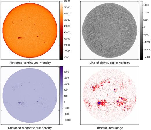
First three panels: SDO/HMI flattened intensity Iflat, line-of sight velocity v (km s−1) for the non-rotating Sun and unsigned radial magnetic flux |Br| (G) of the Sun, observed on 2011 November 10 at 00:01:30 UTC. Last panel: our thresholded image, highlighting faculae (red/lighter shade pixels) and sunspots (blue/darker shade pixels). For this set of observations (representative of the whole run), faculae account for 9 per cent of the total pixel count, while sunspots account for less than 0.4 per cent. The remaining ∼90 per cent of the pixels on the solar disc are magnetically quiet.
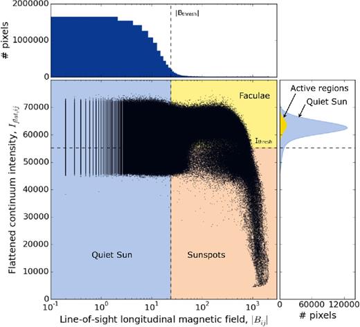
Observed pixel line-of-sight (unsigned) magnetic field strength, |Bobs,ij| (G), as a function of flattened intensity Iflat,ij, for the Sun on 2011 November 10 at 00:01:30 UTC. The top and right histograms show the distributions of |Bobs,ij| and Iflat,ij, respectively. The dashed lines represent the cutoff criteria selected to define the quiet photosphere, faculae and sunspots.
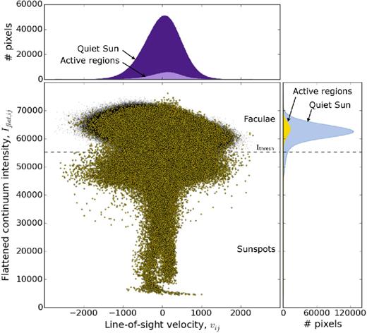
Pixel line-of-sight velocity, vij (in m s−1), as a function of flattened intensity Iflat,ij, for the Sun on 2011 November 10 at 00:01:30 UTC. The top and right histograms show the distributions of vij and Iflat,ij, respectively, in bins of 1000. In the case of active pixels (yellow dots), the line-of-sight velocity is invariant with pixel brightness. For quiet-Sun pixels (black dots), however, brighter pixels are blueshifted while fainter pixels are redshifted: this effect arises from granular motions.
In the main panel of Fig. 5, quiet-Sun pixels are plotted in black, while active-region pixels are overplotted in yellow. The last panel of Fig. 3, which shows the thresholded image according to these Iflat,ij and |Br,ij| criteria, confirms that these thresholding criteria are effective at identifying sunspot and faculae pixels correctly.
Surface velocity flows in sunspot penumbrae and umbrae
The range of velocities in the penumbral pixels (which form the horizontal oval of yellow points just below Ithresh in Fig. 5) is large owing to the Evershed effect (Evershed 1909). The darker umbral pixels have a narrower velocity distribution, allowing the umbral flows that feed the Evershed effect to be resolved into a blueshifted and redshifted velocity component. The much broader range of velocities seen in Fig. 5 for penumbral versus umbral pixels confirms that these velocity flows accelerate with distance from the middle of the spot (Evershed 1909). This effect is highlighted in Fig. 6, which shows a zoom-in on the largest sunspot group in the images of Fig. 3. The Evershed flows are tangential to the surface. They will be most visible for sunspots located away from disc centre, where a larger proportion of them will be directed along our line of sight.
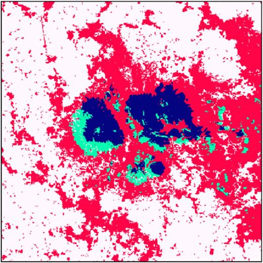
Zoom-in on the largest sunspot group on the approaching hemisphere of the Sun observed on 2011 November 10 at 00:01:30 UTC. Red pixels represent faculae, while the sunspot pixels are colour-coded according to the direction of their velocity flows, thereby revealing the presence of Evershed flows: dark blue pixels are directed towards the observer (v < 0), while light cyan pixels are directed away from the observer (v > 0).
The sunspot group illustrated in Fig. 6 is located near the approaching side of the Sun. The flows in its left half are directed away from the observer, while in its right half they are directed towards the observer.
Decomposing the Sun's RV into individual feature contributions
The total disc-integrated RV of the Sun is the sum of all contributions from the quiet-Sun, sunspot and faculae/plage regions. The ‘quiet’ parts of the Sun's surface are in constant motion due to granulation, while sunspots and faculae induce RV variations via two processes (cf. introduction).
Photometric effect: as the Sun rotates, the presence of dark spots or bright faculae on the solar surface breaks the Doppler balance between the approaching (blueshifted) and receding (redshifted) hemispheres. We calculated the contribution of dark spots and bright faculae separately and our findings confirm those of Meunier et al. (2010a), who found that this residual signal is approximately equal to the photometric contribution from sunspots. We note, however, that this is merely a coincidence arising from the specific geometrical configuration and ratio of sunspots to faculae/plage on the Sun. In other words, this assumption may not be valid for other stars with different spot to faculae configurations and/or filling ratios. We therefore decide to include the effect of faculae in this study (even though it is effectively negligible in the case of the Sun). Because the two contributions are correlated (see Fig. 7), we must account for them in a single term |$\Delta \hat{v}_{\rm phot}$|, which we describe in Section 3.7.2.
Convective effect: sunspots and faculae are strongly magnetized features that inhibit convective motions. Sunspots, which cover a small area of the solar surface and contribute little flux, have a very small contribution. In the case of faculae, however, this contribution is large and is expected to be the dominant contribution to the total solar RV variations (Meunier et al. 2010a,b). We compute this contribution |$\Delta \hat{v}_{\rm conv}$| in Section 3.7.3.
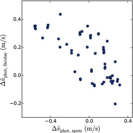
Correlation diagram showing the relationship between the rotational Doppler imbalances resulting from sunspots (horizontal axis) and faculae (vertical axis), if computed separately. The Spearman correlation coefficient is −0.69. The variations are only partially anticorrelated, reflecting both the tendency of faculae to be spatially associated with sunspot groups and the existence of faculae in bright networks not associated with sunspots. The values of these two basis functions are given in the Supplementary Files that are available online.
Velocity contribution of convective motions in quiet-Sun regions
This velocity field is thus averaged over the vertical motions of convection granules on the solar surface. Hot and bright granules rise up to the surface, while cooler and darker fluid sinks back towards the Sun's interior. This process is visible in the main panel of Fig. 5: quiet-Sun pixels (black dots) are clustered in a tilted ellipse. The area of the upflowing granules is larger than that enclosed in the intergranular lanes, and the granules are carrying hotter and thus brighter fluid. This results in a net blueshift, as seen in Fig. 5.
Rotational Doppler imbalance due to dark sunspots and bright faculae
As illustrated in Fig. 7, the photometric effects of sunspots and faculae are quite similar in amplitude and roughly anticorrelated, due to their opposite flux signs. However, because they are not strictly anticorrelated, they sum into a net signal that has an amplitude similar to the photometric effect of sunspots (Meunier et al. 2010a). The value of |$\Delta \hat{v}_{{\rm phot}}$| at each time of the HARPS observations is listed in Table A1. From the SDO images, we derive an rms amplitude of 0.17 m s−1 for this signal, which is smaller than the observational uncertainties of the HARPS velocities. This value is slightly lower than that found by Meunier et al. (2010a) during the peak of the Sun's activity cycle, of 0.42 m s−1, but remains broadly consistent with their results given the small amplitude of this signal.
Suppression of convective blueshift from active regions
The value of |$\Delta \hat{v}_{{\rm conv}}$| at each time of the HARPS observations is listed in Table A1. The rms amplitude of this basis function (unscaled) is 1.30 m s−1, which is consistent with the value of 1.39 m s−1 computed by Meunier et al. (2010a) during the peak of the solar activity cycle.
REPRODUCING THE RV VARIATIONS OF THE SUN
Total RV model
We carry out an optimal scaling procedure in order to determine the scaling factors (A, B, C and S) of each of the contributions, as well as the constant offset RV0 and a constant variance term s2 added in quadrature to the observational errors. This variance term will account for any remaining uncorrelated noise arising from granulation motions. The SDO/HMI images were exposed for 45 s each, while the HARPS observations were exposed for 15 min and binned nightly. We expect these differences to result in a small night-to-night uncorrelated noise contribution. In addition, this variance term will absorb any residual signal of Vesta's axial rotation, which will naturally not be completely sinusoidal.
Agreement between HARPS observations and SDO-derived model
After all the scaling coefficients were determined, we grouped the observations in each night by computing the inverse-variance weighted average for each night. The final model is shown in Fig. 8.
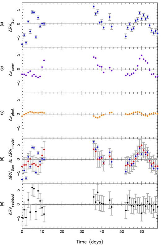
(a) HARPS RV variations of the Sun as a star, ΔRVSun. (b) Scaled basis function for the suppression of convective blueshift, |$\Delta \hat{v}_{\mathrm{conv}}$|, derived from SDO/HMI images. (c) Scaled basis function for the rotational Doppler imbalance due to spots and faculae, |$\Delta \hat{v}_{\mathrm{phot}}$|. (d) Total RV model, ΔRVmodel (red/lighter shade, with errors including additional variance s), overlaid on top of the HARPS RV variations (blue/darker shade points). (e) Residuals obtained after subtracting the model from the observations. All RVs are in m s−1. Note that the scale of the y-axis is different from that used in Fig. 2. The values of these nightly binned time series are provided in the Supplementary Files available online.
We list the best-fitting values of the scaling parameters for each of the basis functions in Table 2. We note that the values of A and B, which represent the difference in response of HARPS and SDO to the Doppler imbalance and the suppression of convective blueshift, differ from unity. The HMI/SDO images are based on measurements of a single spectral line, namely the Fe i 6173 Å line, which may not be representative of the several thousand lines from which the HARPS RVs are derived. The value of |$\Delta \hat{v}_{\mathrm{phot}}$| is determined by the contrast between the magnetic elements (spots, faculae) and the quiet-Sun photosphere. Most of the lines in the HARPS mask lie bluewards of Fe i 6173 Å where the contrast is greater for both types of feature. We therefore expect to have to scale the SDO-derived |$\Delta \hat{v}_{\mathrm{phot}}$| by a factor of order, but greater than, unity. We measure it to be 2.45 ± 2.02; the amplitude of |$\Delta \hat{v}_{\mathrm{phot}}$| is so small that A cannot be distinguished from unity when the additional variance s is taken into account. The strength of the convection inhibition changes with line depth (cf. Gray 2009 and Meunier et al. 2010b). We find that the HARPS response to suppression of granular blueshift is 1.85 ± 0.27 times greater than we predict from SDO.
Best-fitting parameters and rms amplitudes resulting from the optimal scaling procedure.
| Parameter | Value | Basis function | rms amplitude |
|---|---|---|---|
| (unscaled) | |||
| A | 2.45 ± 2.02 | |$\Delta \hat{v}_{{\rm phot}}$| | 0.17 m s−1 |
| B | 1.85 ± 0.27 | |$\Delta \hat{v}_{{\rm conv}}$| | 1.30 m s−1 |
| C | 2.19 ± 0.42 | cos (2π − λ) | 0.74 m s−1 |
| S | 0.55 ± 0.47 | sin (2π − λ) | 0.66 m s−1 |
| RV0 | 99.80 ± 0.28 m s−1 | ||
| s | 2.70 m s−1 |
We show a plot of the observed HARPS RVs (ΔRVSun) versus our SDO-modelled RVs (ΔRVmodel) in Fig. 9, in a similar fashion to fig. 9 of Meunier et al. (2010b). We see good agreement between the data and the model. The Spearman correlation coefficient is 0.64 for the full data set and 0.87 when considering only the second part of the run. This is close to, although not as good as, the correlation coefficient of 0.94 found by Meunier et al. (2010b) between simulated velocities of Meunier et al. (2010a) and MDI/SOHO Dopplergrams.
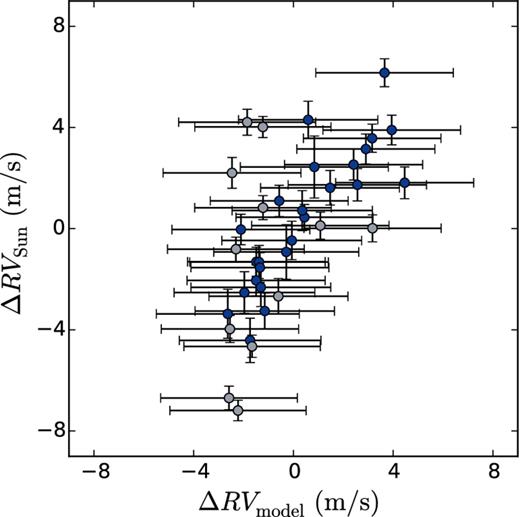
HARPS RV variations of the Sun as a star versus our model derived from SDO/HMI images. Observations from the first part of the run are highlighted in a lighter shade.
Panel (e) of Fig. 8 shows the residuals remaining after subtracting the total model ΔRVmodel from the HARPS observations of the Sun as a star ΔRVSun. We see that the residuals are within the level of the error bars, when considering an extra variance term s of 2.7 m s−1. Maximum-likelihood analysis of the additional uncorrelated noise during the first part of the run (nights 0–11) yields an additional variance with rms amplitude 4.0 m s−1, while the second part (nights 36–68) has an additional noise rms of 1.5 m s−1. As discussed in Section 2.4.2, we attribute the excess scatter in the first block of nights to airmass-dependent guiding errors, which would have been more important in the first part of the run, where the observations within each night were taken at very different airmasses. The additional noise rms of 1.5 m s−1 in the second part of the run is consistent with the rms due to solar granulation and supergranulation, ranging between 0.28 and 1.12 m s−1, as recently found by Meunier et al. (2015).
Relative importance of suppression of convective blueshift and rotational velocity imbalance
We see that the activity-induced RV variations of the Sun are well reproduced by a scaled sum of the two basis functions, |$\hat{v}_{{\rm conv}}$| and |$\hat{v}_{{\rm phot}}$| (shown in panels (b) and (c) of Fig. 8, respectively). As previously predicted by Meunier et al. (2010a), we find that the suppression of convective blueshift plays a dominant role (rms of 2.40 m s−1). This was also found to be the case for CoRoT-7, a main-sequence G9 star with a rotation period comparable to that of the Sun (Haywood et al. 2014). The relatively low amplitude of the modulation induced by sunspot flux blocking (rms of 0.17 m s−1) is expected in slowly rotating stars with a low v sin i (Desort et al. 2007).
Zero-point of HARPS
The wavelength adjustments that were applied to the HARPS RVs were based on precise prior dynamical knowledge of the rate of change of distance between the Earth and Vesta, and between Vesta and the Sun. The offset RV0 = 99.80 ± 0.28 m s−1 thus represents the zero-point of the HARPS instrument, including the mean granulation blueshift for the Sun. A previous study of integrated sunlight reflected by the Moon, by Molaro et al. (2013), determined a value of 102.2 ± 0.86 m s−1, which is significantly larger than our value. They did not account for the effect of sunspots and faculae, however, so their result could be affected by activity-induced solar variations at that time.
TOWARDS BETTER PROXIES FOR RV OBSERVATIONS
Spatial distributions of sunspots and faculae
Aigrain, Pont & Zucker (2012) have shown that it is possible to predict the rotational Doppler imbalance due to photospheric surface brightness inhomogeneities from a simultaneous high-precision optical light curve. If one further assumes that faculae/plage regions are co-spatial with spot groups, then they can also predict the form of the RV variation caused by suppression of granular blueshift. A recent analysis of the active host star CoRoT-7 by Haywood et al. (2014) modelled activity-induced RV variations via the FF′ method of Aigrain et al. (2012). The predicted Doppler imbalance was much smaller than the observed activity-driven RV variations. The associated suppression of convective blueshift was of larger amplitude than, and partially correlated with, the observed RVs. The residuals, however, had a similar amplitude and shared the covariance properties of the star's (simultaneous) light curve.
The present study provides a natural explanation of this mismatch: on the Sun, the faculae are not perfectly co-spatial with sunspot groups. Indeed, Fig. 7 shows us that the location of sunspot groups gives an incomplete prediction of the facular coverage. Since the suppression of granular blueshift is the dominant process at play in slowly rotating stars such as CoRoT-7 and the Sun, it is therefore important to develop proxies that are directly sensitive to the distribution of faculae on the stellar surface.
Correlations between RV and traditional activity indicators
Fig. 10 presents the correlations between ΔRVSun, |$\Delta \hat{v}_{{\rm conv}}$| and the following activity indicators: the full-disc magnetic flux |$|\hat{B}_{\rm obs}|$| and filling factor f computed from the SDO/HMI images, and the observed FWHM, BIS and |$\log (R^{\prime }_{HK})$| derived from the HARPS DRS reduction pipeline. We computed the Spearman correlation coefficient to get a measure of the degree of monotone correlation between each variable (the correlation between two variables is not necessarily linear, for example between RV and BIS). The coefficients are displayed in each panel of Fig. 10, both including and excluding the observations made in the first part of the run, which show a lot of intra-night scatter.
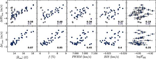
Correlation plots of the nightly averaged HARPS RV variations of the Sun as a star ΔRVSun and suppression of convective blueshift |$\Delta \hat{v}_{{\rm conv}}$| against (from left to right): the disc-averaged observed magnetic flux |$|\hat{B}_{\rm obs}|$| (G), filling factor f (per cent), FWHM (km s−1), BIS (m s−1) and |$\log (R^{\prime }_{HK})$|. Observations from the first part of the run are highlighted in a lighter shade. Spearman correlation coefficients are displayed in the bottom-right corner of each panel: for the full observing run (in bold and black), and for the second part of the run only (in blue).
We do not show similar correlation plots for |$\Delta \hat{v}_{{\rm phot}}$| because we do not find any significant correlations with any of the activity indicators; this is expected since |$\Delta \hat{v}_{{\rm phot}}$| is such that it crosses zero when the surface covered by spots and/or faculae is at a maximum, i.e. when they are in the middle of the stellar disc (|$\Delta \hat{v}_{{\rm phot}}$| is of course still related to |$|\hat{B}_{\rm obs}|$|, the FWHM, BIS and |$\log (R^{\prime }_{HK})$|, but the Spearman coefficient is close to zero).
We note that the relatively weak correlation between the observed RVs and the BIS is not completely unexpected in the case of the Sun, which has a vsin i of about 2 km s−1. The line profile distortions induced by solar activity, including those measured by the BIS, will therefore be smaller than the resolution of HARPS that is close to 2.5 km s−1. In other words, the resolution of HARPS is not adequate to fully resolve the BIS variations in a star rotating as slowly as the Sun, which could reduce the correlation coefficients computed with the BIS.
We find a relatively weak correlation between the observed RVs and the chromospheric flux index |$\log (R^{\prime }_{HK})$|, with a Spearman correlation coefficient of 0.26 for the second half of the run (0.18 for the full run).
Although naively one might expect |$\log (R^{\prime }_{HK})$| to be a good predictor of plage filling factor, and hence of the convective RV component, there are several physical factors that might reasonably be expected to degrade the correlation over short time-scales (our data set spans two to three solar rotations). Foreshortening and limb darkening affect the Ca ii H&K emission cores and the brightness-weighted line-of-sight granular velocities in different ways. Near the limb, the Ca ii emission in plages originates in higher, hotter regions of the chromosphere and remains bright. The limb darkening of facular pixels is less than that of quiet-Sun pixels, but near the limb the line-of-sight component of the radial motion of bright granule cores is reduced by foreshortening. The disc-averaged line-of-sight magnetic field strength is attenuated by both foreshortening and limb darkening in approximately the same way as the radial motion of the granular flow. This may explain why, even though the RVs and |$\log (R^{\prime }_{HK})$| values were measured simultaneously from the same spectra, the correlation between the variations in |$\log (R^{\prime }_{HK})$| and suppression of granular blueshift appears weak. In their study of long-term solar RV variations spanning over 8 years, Lanza et al. (2016) find a stronger correlation between |$\log (R^{\prime }_{HK})$| and RV variations, with a Spearman coefficient of 0.357. This positive correlation is in agreement with previous studies of quiet late-type stars (Lovis et al. 2011; Gomes da Silva et al. 2012), and shows that the |$\log (R^{\prime }_{HK})$| may be a more useful proxy for long-term RV variations induced by the stellar magnetic cycle.
We note that in Fig. 10, the variations in |$\log (R^{\prime }_{HK})$| look similar to the variations in RV, except that they are shifted by a few days (this is especially noticeable towards the end of the run). The reality and origin of this shift will be the subject of future studies, thanks to the wealth of Sun as a star RV observations that are currently being gathered by the solar telescope at HARPS-N.
Disc-averaged observed magnetic flux |$|\hat{B}_{\rm obs}|$|
The values at the time of each HARPS observation are listed in Table A1. The variations in |$|\hat{B}_{\rm obs}|$| are shown in panel (b) of Fig. 11, together with the nightly averaged HARPS RV variations of the Sun as a star, in panel (a). We see that the variations in the disc-averaged magnetic flux are in phase with the RV variations, despite the scatter in RV in the first part of the run (discussed in Section 2.4.2). If we only consider the observations in the second part of the run, the Spearman correlation coefficient between ΔRVSun and |$|\hat{B}_{\rm obs}|$| is 0.80 (see Fig. 10). The correlation is stronger between |$\hat{v}_{{\rm conv}}$| and |$|\hat{B}_{\rm obs}|$|, with a correlation coefficient of 0.87. This is expected since magnetized areas are known to suppress convective blueshift (see Meunier et al. 2010a,b).
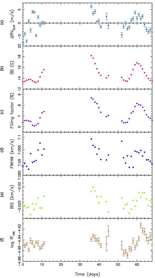
(a) HARPS RV variations of the Sun as a star. (b and c) Time series of the disc-averaged line-of-sight magnetic flux |$|\hat{B}_{\rm obs}|$| and filling factor f, respectively, determined from the SDO/HMI magnetograms. (d–f) Time series of the FWHM, BIS and |$\log (R^{\prime }_{HK})$|, respectively, determined from the HARPS DRS reduction pipeline. The values of these nightly binned time series are provided in the Supplementary Files available online.
We note that these observations were taken close to the solar cycle maximum, during which the solar photosphere was mostly dominated by a few large sunspot groups (surrounded by facular networks). Meunier et al. (2010b) found that the convective shift attenuation is greater in larger structures, since they contain a stronger magnetic field. The relationship between convective shift attenuation and magnetic field, however, is not linear. We thus expect larger RV variations for a few large active regions than when the Sun is in a phase of lower magnetic activity, when the photosphere might be dominated by several smaller structures, even though they would still give the same total flux. In fact, Lanza et al. (2016) find a much weaker correlation between the mean total magnetic flux measured by the Synoptic Optical Long-term Investigations of the Sun (SOLIS) Vector Spectromagnetograph (VSM) instrument and RV (Spearman correlation coefficient of 0.131) over their 8-yr data set, which spans both active and less active phases of the solar cycle.
When compared against correlations with the traditional spectroscopic activity indicators (the FWHM, BIS and |$\log (R^{\prime }_{HK})$|), we see that the disc-averaged magnetic flux |$|\hat{B}_{\rm obs}|$| is a much more effective predictor of activity-induced RV variations, over the time-scale of a few rotation periods. The averaged magnetic flux may therefore be a useful proxy for activity-driven RV variations as it should map on to areas of strong magnetic fields, which suppress the Sun's convective blueshift. The line-of-sight magnetic flux density and filling factor on the visible hemisphere of a star can be measured from the Zeeman broadening of magnetically sensitive lines (Robinson 1980; Reiners et al. 2013). Their product gives the disc-averaged flux density that we are deriving from the solar images. We note that such measurements are still very difficult to make for other stars than the Sun, because the Zeeman splitting of magnetically sensitive lines is so small that the technique can only be applied to bright, slowly rotating stars. Fortunately, such stars are also the best targets for planet searches.
Magnetic filling factor f
CONCLUSION
In the present analysis, we decomposed activity-induced RV variations into identifiable contributions from sunspots, faculae and granulation, based on Sun as a star RV variations deduced from HARPS spectra of the bright asteroid Vesta and high spatial resolution images in the Fe i 6173 Å line taken with the HMI instrument aboard the SDO. We find that the RV variations induced by solar activity are mainly caused by the suppression of convective blueshift from magnetically active regions, while the flux deficit incurred by the presence of sunspots on the rotating solar disc only plays a minor role. We further compute the disc-averaged line-of-sight magnetic flux and show that although we cannot yet measure it with precision on other stars at present, it is a very good proxy for activity-driven RV variations, much more so than the FWHM and BIS of the cross-correlation profile, and the Ca ii H&K activity index. These findings are in agreement with the previous works of Meunier et al. (2010a,b).
In addition to the existing 2011 HARPS observations of sunlight scattered off Vesta, there will soon be a wealth of direct solar RV measurements taken with HARPS-N, which will be regularly fed sunlight through a small 2-inch telescope developed specifically for this purpose. A prototype for this is currently being commissioned at HARPS-N (see Dumusque et al. 2015; Glenday et al., in preparation). Gaining a deeper understanding of the physics at the heart of activity-driven RV variability will ultimately enable us to better model and remove this contribution from RV observations, thus revealing the planetary signals.
We wish to thank the referee for their thoughtful comments, which have greatly helped improve the analysis presented in this paper. RDH gratefully acknowledges STFC studentship grant number ST/J500744/1, and a grant from the John Templeton Foundation. The opinions expressed in this publication are those of the authors and do not necessarily reflect the views of the John Templeton Foundation. ACC and RF acknowledge support from STFC consolidated grants numbers ST/J001651/1 and ST/M001296/1. JL acknowledges support from NASA Origins of the Solar System grant No. NNX13AH79G and from STFC grant ST/M001296/1. The Solar Dynamics Observatory was launched by NASA on 2011 February 11, as part of the Living With A Star programme. This research has made use of NASA's Astrophysics Data System Bibliographic Services. We also used data from Haywood et al. (2016).
Plages are formed in the upper photosphere, chromosphere and upper layers of the stellar atmosphere (Lean 1997; Murdin 2002). They are not part of the lower photosphere, where the continuum absorption lines originate, from which the RV of a star is measured; however, plage regions do map closely to faculae and sunspots (Schrijver 2002; Hall 2008).
Solar System Dynamics Group, Horizons On-Line Ephemeris System, 4800 Oak Grove Drive, Jet Propulsion Laboratory, Pasadena, CA 91109 USA – Information: http://ssd.jpl.nasa.gov/, [email protected]
HMI data products can be downloaded online via the Joint Science Operations Center website: http://jsoc.stanford.edu.
Source code available at http://hesperia.gsfc.nasa.gov/ssw/gen/idl/solar/
REFERENCES
SUPPORTING INFORMATION
Additional Supporting Information may be found in the online version of this article:
Based on observations made with the HARPS instrument on the 3.6 m telescope under the programme ID 088.C-0323 at Cerro La Silla (Chile) and the Helioseismic and Magnetic Imager on board the Solar Dynamics Observatory. The HARPS observations, together with tables for the results presented in this paper, are available in electronic format at: The SDO/HMI images can be downloaded from http://jsoc.stanford.edu
http://dx.doi.org/10.17630/bb43e6a3-72e0-464c-9fdd-fbe5d3e56a09
Please note: Oxford University Press are not responsible for the content or functionality of any supporting materials supplied by the authors. Any queries (other than missing material) should be directed to the corresponding author for the article.
APPENDIX A:
HARPS 2011–2012 data for the asteroid Vesta, processed by the HARPS pipeline with the correct barycentric RV and accounting for the relativistic correction, and SDO-derived quantities resulting from our analysis. From left to right are given: Julian date (flux-weighted mid-exposure times of observation), RV, the estimated error σRV on the RV measurement, the full width at half-maximum (FWHM) and the line bisector of (BIS) of the cross-correlation function (as defined in Queloz et al. 2001), the Ca ii H&K activity indicator log(|$R^{\prime }_{HK}$|) and its error |$\sigma _{\log (R^{\prime }_{HK})}$|, the time lag Δt between the HARPS observations and the time at which SDO observed the same hemisphere of the Sun, the apparent planetographic longitude of Vesta λ, the values of the basis functions for the sunspot velocity signal, |$\hat{v}_{{\rm phot}}$| and the suppression of granular blueshift, |$\hat{v}_{{\rm conv}}$|, the full-disc magnetic flux |$|\hat{B}_{\rm obs}|$| and the filling factor of magnetic regions f both computed from the SDO images. An expanded version of this table, together with all Supplementary Files, is available electronically at http://dx.doi.org/10.17630/bb43e6a3-72e0-464c-9fdd-fbe5d3e56a09.
| Julian date | RV | σRV | FWHM | BIS | |$\log (R^{\prime }_{HK}$|) | |$\sigma _{\log (R^{\prime }_{HK})}$| | Δt | λ | |$\hat{v}_{{\rm phot}}$| | |$\hat{v}_{{\rm conv}}$| | |$|\hat{B}_{\rm obs}|$| | f |
|---|---|---|---|---|---|---|---|---|---|---|---|---|
| (MJDmid_UTC) | (km s−1) | (km s−1) | (km s−1) | (km s−1) | (d) | (deg) | (m s−1) | (m s−1) | (G) | (per cent) | ||
| 2455834.48296192 | 0.085 70 | 0.000 43 | 7.089 02 | − 0.024 17 | − 4.9411 | 0.0024 | 2.8365 | 143.99 | − 0.122 949 | 6.612 382 | 13.390 075 | 6.442 092 |
| 2455834.61321887 | 0.099 36 | 0.000 39 | 7.0883 | − 0.025 59 | − 4.9435 | 0.0019 | 2.8451 | 351.75 | − 0.122 949 | 6.612 382 | 13.390 075 | 6.442 092 |
| 2455835.53355275 | 0.094 77 | 0.000 49 | 7.089 03 | − 0.024 78 | − 4.9513 | 0.0028 | 2.8901 | 39.73 | − 0.372 071 | 6.728 378 | 13.461 877 | 6.553 660 |
| 2455835.66225392 | 0.099 36 | 0.000 60 | 7.090 69 | − 0.024 77 | − 4.9498 | 0.0044 | 2.9002 | 247.49 | − 0.369 973 | 6.800 018 | 13.456 769 | 6.559 029 |
| 2455836.50488464 | 0.084 31 | 0.000 46 | 7.089 78 | − 0.024 77 | − 4.9450 | 0.0027 | 2.9396 | 171.93 | − 0.148 130 | 6.458 323 | 13.693 823 | 6.750 327 |
| 2455836.63463460 | 0.102 54 | 0.000 47 | 7.087 21 | − 0.025 89 | − 4.9506 | 0.0029 | 2.9487 | 19.69 | − 0.149 324 | 6.451 065 | 13.612 058 | 6.682 767 |
| 2455837.58225198 | 0.099 16 | 0.000 43 | 7.086 32 | − 0.024 37 | − 4.9575 | 0.0026 | 2.9941 | 112.57 | − 0.062 027 | 7.066 728 | 13.760 690 | 6.785 311 |
| 2455837.66801992 | 0.101 48 | 0.000 54 | 7.089 11 | − 0.026 32 | − 4.9597 | 0.0041 | 3.0056 | 252.95 | − 0.062 027 | 7.066 728 | 13.760 690 | 6.785 311 |
| 2455838.56557661 | 0.095 52 | 0.000 65 | 7.093 28 | − 0.026 98 | − 4.9373 | 0.0043 | 3.0525 | 261.60 | − 0.104 478 | 7.448 517 | 13.797 603 | 6.798 914 |
| 2455838.67384272 | 0.099 25 | 0.000 77 | 7.0939 | − 0.027 17 | − 4.9475 | 0.0061 | 3.0623 | 81.28 | − 0.104 478 | 7.448 517 | 13.797 603 | 6.798 914 |
| 2455839.56369186 | 0.106 00 | 0.000 49 | 7.090 53 | − 0.023 31 | − 4.9480 | 0.0031 | 3.1099 | 78.70 | 0.282 247 | 6.290 580 | 13.538 572 | 6.711 449 |
| 2455839.66500316 | 0.101 44 | 0.000 54 | 7.089 58 | − 0.025 47 | − 4.9404 | 0.0038 | 3.1058 | 241.53 | 0.282 247 | 6.290 580 | 13.538 572 | 6.711 449 |
| 2455840.54096382 | 0.101 81 | 0.000 42 | 7.090 45 | − 0.025 73 | − 4.9519 | 0.0024 | 3.1535 | 216.48 | 0.492 760 | 6.355 797 | 13.337 171 | 6.545 630 |
| 2455841.51821591 | 0.097 43 | 0.000 44 | 7.0908 | − 0.024 34 | − 4.9443 | 0.0023 | 3.2110 | 359.87 | 0.548 444 | 6.054 414 | 13.267 717 | 6.419 010 |
| 2455842.54067654 | 0.101 56 | 0.000 58 | 7.093 98 | − 0.023 31 | − 4.9419 | 0.0041 | 3.2579 | 210.63 | 0.285 453 | 5.964 030 | 13.453 311 | 6.502 014 |
| 2455842.64940682 | 0.102 21 | 0.000 65 | 7.096 29 | − 0.022 21 | − 4.9521 | 0.0051 | 3.2673 | 30.31 | 0.285 453 | 5.964 030 | 13.453 311 | 6.502 014 |
| 2455843.53446953 | 0.101 35 | 0.000 42 | 7.097 55 | − 0.024 79 | − 4.9529 | 0.0023 | 3.3128 | 16.47 | 0.289 295 | 6.042 467 | 14.255 929 | 7.096 244 |
| 2455843.66473254 | 0.097 22 | 0.000 57 | 7.097 89 | − 0.0264 | − 4.9598 | 0.0043 | 3.3214 | 229.83 | 0.289 295 | 6.042 467 | 14.255 929 | 7.096 244 |
| 2455844.53056656 | 0.096 56 | 0.000 58 | 7.090 06 | − 0.024 79 | − 4.9538 | 0.0039 | 3.3722 | 187.91 | 0.338 963 | 7.427 578 | 15.036 871 | 7.600 587 |
| 2455844.66179197 | 0.102 92 | 0.000 50 | 7.095 19 | − 0.0258 | − 4.9513 | 0.0033 | 3.3799 | 41.27 | 0.412 640 | 7.942 586 | 15.167 705 | 7.742 510 |
| 2455845.54569082 | 0.101 43 | 0.000 53 | 7.093 54 | − 0.0214 | − 4.9472 | 0.0032 | 3.4265 | 33.04 | 0.214 037 | 9.072 355 | 15.656 077 | 8.091 010 |
| 2455845.65206487 | 0.098 30 | 0.000 54 | 7.097 19 | − 0.023 43 | − 4.9456 | 0.0036 | 3.4313 | 201.48 | 0.147 598 | 9.104 808 | 15.530 288 | 7.938 438 |
| 2455870.51420322 | 0.108 43 | 0.000 59 | 7.098 49 | − 0.019 02 | − 4.9355 | 0.0032 | 4.7844 | 86.70 | − 0.230 017 | 9.870 595 | 18.187 723 | 9.696 133 |
| 2455870.52215421 | 0.107 01 | 0.000 53 | 7.101 07 | − 0.021 57 | − 4.9399 | 0.0035 | 4.7834 | 97.93 | − 0.230 017 | 9.870 595 | 18.187 723 | 9.696 133 |
| 2455870.53060607 | 0.103 79 | 0.000 53 | 7.098 26 | − 0.022 32 | − 4.9419 | 0.0036 | 4.7819 | 109.16 | − 0.230 017 | 9.870 595 | 18.187 723 | 9.696 133 |
| 2455871.50280525 | 0.102 50 | 0.000 61 | 7.093 61 | − 0.018 83 | − 4.9341 | 0.0033 | 4.8375 | 241.14 | − 0.247 643 | 9.628 828 | 17.731 211 | 9.520 507 |
| 2455871.51026399 | 0.101 90 | 0.000 53 | 7.097 64 | − 0.020 95 | − 4.9334 | 0.0033 | 4.8370 | 252.37 | − 0.247 643 | 9.628 828 | 17.731 211 | 9.520 507 |
| 2455871.51752074 | 0.102 79 | 0.000 53 | 7.098 29 | − 0.020 04 | − 4.9307 | 0.0033 | 4.8366 | 269.21 | − 0.247 643 | 9.628 828 | 17.731 211 | 9.520 507 |
| 2455872.49503353 | 0.106 38 | 0.001 77 | 7.103 66 | − 0.023 63 | − 4.8856 | 0.0193 | 4.8869 | 46.81 | − 0.217 090 | 8.539 591 | 16.708 896 | 8.931 849 |
| 2455872.50361680 | 0.107 06 | 0.000 63 | 7.098 57 | − 0.0206 | − 4.9459 | 0.0044 | 4.8853 | 63.65 | − 0.212 479 | 8.339 659 | 16.718 279 | 8.928 224 |
| 2455872.51065080 | 0.104 33 | 0.000 66 | 7.093 74 | − 0.021 82 | − 4.9417 | 0.0046 | 4.8852 | 74.88 | − 0.232 778 | 8.259 415 | 16.704 289 | 8.916 693 |
| 2455872.51832551 | 0.104 31 | 0.000 66 | 7.094 74 | − 0.020 18 | − 4.9297 | 0.0044 | 4.8914 | 86.10 | − 0.218 351 | 8.044 784 | 16.715 321 | 8.926 018 |
| 2455873.50406872 | 0.098 70 | 0.000 50 | 7.091 24 | − 0.022 93 | − 4.9400 | 0.0030 | 4.9404 | 240.54 | − 0.159 657 | 7.999 471 | 15.740 116 | 8.388 542 |
| 2455873.51131777 | 0.099 37 | 0.000 50 | 7.092 52 | − 0.021 97 | − 4.9425 | 0.0031 | 4.9401 | 251.76 | − 0.149 055 | 8.115 433 | 15.749 984 | 8.389 838 |
| 2455873.51863681 | 0.099 33 | 0.000 51 | 7.096 35 | − 0.022 45 | − 4.9380 | 0.0030 | 4.9397 | 262.99 | − 0.137 447 | 8.065 520 | 15.735 783 | 8.370 678 |
| 2455874.50355099 | 0.101 33 | 0.000 77 | 7.096 52 | − 0.023 86 | − 4.9467 | 0.0051 | 4.9964 | 57.42 | − 0.289 008 | 8.449 905 | 15.011 817 | 7.870 854 |
| 2455874.51074342 | 0.102 94 | 0.000 74 | 7.092 61 | − 0.023 14 | − 4.9402 | 0.0057 | 4.9962 | 68.65 | − 0.305 588 | 8.072 379 | 14.993 994 | 7.858 010 |
| 2455874.51805876 | 0.101 32 | 0.000 89 | 7.097 96 | − 0.025 44 | − 4.9379 | 0.0069 | 4.9958 | 79.87 | − 0.305 588 | 8.072 379 | 14.993 994 | 7.858 010 |
| 2455875.50408302 | 0.098 39 | 0.000 58 | 7.089 79 | − 0.024 18 | − 4.9544 | 0.0040 | 5.0515 | 234.30 | − 0.160 578 | 7.051 506 | 14.539 260 | 7.545 515 |
| 2455875.51155021 | 0.096 71 | 0.000 57 | 7.091 51 | − 0.023 84 | − 4.9472 | 0.0039 | 5.0509 | 245.52 | − 0.160 578 | 7.051 506 | 14.539 260 | 7.545 515 |
| 2455875.51886866 | 0.096 45 | 0.000 58 | 7.092 36 | − 0.019 25 | − 4.9500 | 0.0040 | 5.0506 | 256.75 | − 0.160 578 | 7.051 506 | 14.539 260 | 7.545 515 |
| 2455878.50606288 | 0.104 81 | 0.001 23 | 7.093 06 | − 0.023 84 | − 4.9368 | 0.0129 | 5.2162 | 44.91 | 0.239 367 | 7.862 843 | 14.083 289 | 7.241 949 |
| 2455878.51386630 | 0.103 96 | 0.001 25 | 7.087 15 | − 0.020 17 | − 4.9521 | 0.0137 | 5.2153 | 56.14 | 0.219 175 | 7.727 767 | 14.087 698 | 7.262 066 |
| 2455878.52076438 | 0.103 24 | 0.001 20 | 7.092 72 | − 0.026 94 | − 4.9529 | 0.0128 | 5.2153 | 67.36 | 0.215 755 | 7.792 477 | 14.102 572 | 7.257 334 |
| 2455879.50702795 | 0.097 25 | 0.001 12 | 7.094 57 | − 0.025 22 | − 4.9197 | 0.0103 | 5.2777 | 227.38 | 0.232 115 | 7.128 572 | 14.466 632 | 7.447 019 |
| 2455879.51427708 | 0.097 05 | 0.001 07 | 7.089 51 | − 0.028 34 | − 4.9360 | 0.0100 | 5.2774 | 238.61 | 0.230 304 | 6.983 342 | 14.483 479 | 7.457 781 |
| 2455879.52152229 | 0.097 81 | 0.001 05 | 7.094 96 | − 0.025 36 | − 4.9146 | 0.0093 | 5.2771 | 249.84 | 0.232 562 | 7.438 171 | 14.526 323 | 7.492 319 |
| 2455886.55971131 | 0.096 68 | 0.000 85 | 7.099 98 | − 0.021 19 | − 4.9537 | 0.0073 | 5.6625 | 109.52 | 0.232 784 | 6.416 208 | 14.173 657 | 6.983 742 |
| 2455886.56696080 | 0.094 96 | 0.000 86 | 7.094 83 | − 0.023 48 | − 4.9481 | 0.0075 | 5.6622 | 120.75 | 0.232 784 | 6.416 208 | 14.173 657 | 6.983 742 |
| 2455886.57392844 | 0.092 57 | 0.000 93 | 7.100 74 | − 0.0237 | − 4.9477 | 0.0086 | 5.6622 | 131.98 | 0.232 784 | 6.416 208 | 14.173 657 | 6.983 742 |
| 2455887.52342644 | 0.096 87 | 0.000 60 | 7.090 76 | − 0.023 92 | − 4.9636 | 0.0042 | 5.7196 | 224.60 | 0.254 368 | 6.578 471 | 13.681 434 | 6.611 017 |
| 2455887.53095415 | 0.097 45 | 0.000 67 | 7.091 91 | − 0.026 85 | − 4.9726 | 0.0052 | 5.7190 | 235.83 | 0.254 368 | 6.578 471 | 13.681 434 | 6.611 017 |
| 2455887.53806579 | 0.096 16 | 0.000 72 | 7.093 53 | − 0.026 17 | − 4.9578 | 0.0056 | 5.7189 | 247.06 | 0.254 368 | 6.578 471 | 13.681 434 | 6.611 017 |
| 2455888.52593242 | 0.101 10 | 0.000 60 | 7.090 39 | − 0.026 13 | − 4.9661 | 0.0043 | 5.7727 | 47.04 | 0.157 666 | 6.316 140 | 13.525 647 | 6.498 637 |
| 2455888.53317611 | 0.101 58 | 0.000 59 | 7.088 31 | − 0.022 24 | − 4.9623 | 0.0043 | 5.7724 | 58.27 | 0.157 666 | 6.316 140 | 13.525 647 | 6.498 637 |
| 2455888.54049630 | 0.101 75 | 0.000 62 | 7.090 83 | − 0.025 48 | − 4.9577 | 0.0047 | 5.7720 | 69.50 | 0.157 666 | 6.316 140 | 13.525 647 | 6.498 637 |
| 2455889.52578074 | 0.097 55 | 0.000 60 | 7.091 31 | − 0.026 11 | − 4.9642 | 0.0045 | 5.8284 | 223.87 | 0.183 892 | 6.607 664 | 13.455 927 | 6.430 930 |
| 2455889.53310116 | 0.096 01 | 0.000 60 | 7.093 05 | − 0.024 11 | − 4.9633 | 0.0046 | 5.8280 | 235.10 | 0.183 892 | 6.607 664 | 13.455 927 | 6.430 930 |
| 2455889.54034195 | 0.094 61 | 0.000 65 | 7.093 77 | − 0.022 42 | − 4.9796 | 0.0054 | 5.8277 | 246.32 | 0.183 892 | 6.607 664 | 13.455 927 | 6.430 930 |
| 2455890.50917526 | 0.100 97 | 0.000 59 | 7.088 86 | − 0.028 67 | − 4.9505 | 0.0040 | 5.8867 | 12.62 | 0.079 914 | 6.820 067 | 13.946 109 | 6.891 653 |
| 2455890.51649149 | 0.100 74 | 0.000 58 | 7.087 63 | − 0.026 59 | − 4.9564 | 0.0040 | 5.8863 | 23.85 | 0.079 914 | 6.820 067 | 13.946 109 | 6.891 653 |
| 2455890.52382222 | 0.099 96 | 0.000 59 | 7.087 79 | − 0.024 85 | − 4.9611 | 0.0042 | 5.8859 | 35.08 | 0.079 914 | 6.820 067 | 13.946 109 | 6.891 653 |
| 2455891.52246765 | 0.099 41 | 0.000 60 | 7.091 51 | − 0.025 35 | − 4.9591 | 0.0044 | 5.9428 | 211.90 | 0.079 914 | 6.820 067 | 13.946 109 | 6.891 653 |
| 2455891.52978471 | 0.099 21 | 0.000 63 | 7.0924 | − 0.025 49 | − 4.9649 | 0.0049 | 5.9424 | 223.12 | − 0.128 128 | 7.724 229 | 15.031 973 | 7.761 893 |
| 2455891.53703495 | 0.098 40 | 0.000 63 | 7.093 53 | − 0.026 16 | − 4.9482 | 0.0049 | 5.9421 | 234.35 | − 0.128 128 | 7.724 229 | 15.031 973 | 7.761 893 |
| 2455892.52735539 | 0.103 98 | 0.000 61 | 7.086 42 | − 0.022 54 | − 4.9442 | 0.0045 | 5.9935 | 34.33 | 0.250 746 | 8.037 871 | 15.638 486 | 7.970 436 |
| 2455892.53453612 | 0.103 58 | 0.000 79 | 7.091 45 | − 0.024 41 | − 4.9370 | 0.0068 | 5.9932 | 45.55 | 0.239 745 | 8.154 407 | 15.602 640 | 7.956 911 |
| 2455892.54214391 | 0.102 47 | 0.000 69 | 7.0878 | − 0.023 79 | − 4.9422 | 0.0054 | 5.9995 | 62.40 | 0.239 745 | 8.154 407 | 15.602 640 | 7.956 911 |
| 2455893.51437423 | 0.100 22 | 0.000 59 | 7.095 16 | − 0.024 93 | − 4.9440 | 0.0040 | 6.0551 | 194.30 | 0.178 788 | 9.501 673 | 16.492 246 | 8.578 127 |
| 2455893.52626540 | 0.102 39 | 0.000 57 | 7.091 83 | − 0.025 14 | − 4.9578 | 0.0040 | 6.0501 | 211.14 | 0.178 788 | 9.501 673 | 16.492 246 | 8.578 127 |
| 2455893.53359078 | 0.102 28 | 0.000 60 | 7.096 83 | − 0.024 59 | − 4.9607 | 0.0044 | 6.0497 | 222.37 | 0.178 788 | 9.501 673 | 16.492 246 | 8.578 127 |
| 2455894.50541095 | 0.102 65 | 0.000 59 | 7.094 96 | − 0.023 71 | − 4.9499 | 0.0041 | 6.0988 | 354.27 | − 0.143 119 | 10.188 700 | 16.843 670 | 8.978 122 |
| 2455894.51266019 | 0.104 00 | 0.000 62 | 7.093 07 | − 0.023 55 | − 4.9416 | 0.0044 | 6.1054 | 5.49 | − 0.143 119 | 10.188 700 | 16.843 670 | 8.978 122 |
| 2455894.52011844 | 0.105 48 | 0.000 68 | 7.094 66 | − 0.023 04 | − 4.9486 | 0.0052 | 6.1049 | 16.72 | − 0.143 119 | 10.188 700 | 16.843 670 | 8.978 122 |
| 2455895.51190055 | 0.098 55 | 0.000 58 | 7.0944 | − 0.0217 | − 4.9341 | 0.0038 | 6.1617 | 182.30 | − 0.219 694 | 9.459 038 | 16.678 771 | 8.985 445 |
| 2455895.51928533 | 0.100 14 | 0.000 61 | 7.093 07 | − 0.022 48 | − 4.9339 | 0.0041 | 6.1613 | 193.53 | − 0.219 694 | 9.459 038 | 16.678 771 | 8.985 445 |
| 2455895.52668202 | 0.103 85 | 0.000 60 | 7.094 09 | − 0.020 13 | − 4.9456 | 0.0041 | 6.1608 | 204.76 | − 0.219 694 | 9.459 038 | 16.678 771 | 8.985 445 |
| 2455896.51221054 | 0.103 11 | 0.000 62 | 7.095 55 | − 0.0246 | − 4.9082 | 0.0042 | 6.2170 | 359.11 | − 0.118 240 | 9.149 870 | 16.324 338 | 8.893 371 |
| 2455896.51945075 | 0.104 02 | 0.000 64 | 7.0943 | − 0.021 61 | − 4.9219 | 0.0044 | 6.2167 | 10.34 | − 0.118 240 | 9.149 870 | 16.324 338 | 8.893 371 |
| 2455896.52676887 | 0.104 50 | 0.000 65 | 7.0945 | − 0.0215 | − 4.9086 | 0.0045 | 6.2163 | 21.56 | − 0.118 240 | 9.149 870 | 16.324 338 | 8.893 371 |
| 2455897.51313557 | 0.098 05 | 0.000 57 | 7.0929 | − 0.021 41 | − 4.9279 | 0.0041 | 6.2716 | 175.91 | 0.310 313 | 8.521 387 | 15.731 010 | 8.518 003 |
| 2455897.52017185 | 0.101 99 | 0.000 61 | 7.090 74 | − 0.020 29 | − 4.9207 | 0.0045 | 6.2715 | 187.14 | 0.310 313 | 8.521 387 | 15.731 010 | 8.518 003 |
| 2455897.52797234 | 0.101 03 | 0.000 66 | 7.094 31 | − 0.022 93 | − 4.9178 | 0.0049 | 6.2776 | 203.98 | 0.310 313 | 8.521 387 | 15.731 010 | 8.518 003 |
| 2455898.51251923 | 0.100 34 | 0.000 76 | 7.094 42 | − 0.025 29 | − 4.9139 | 0.0059 | 6.3278 | 352.71 | 0.208 771 | 7.346 064 | 15.023 078 | 7.994 100 |
| 2455898.51955262 | 0.102 92 | 0.000 74 | 7.095 72 | − 0.020 88 | − 4.9290 | 0.0060 | 6.3277 | 3.94 | 0.193 525 | 7.375 161 | 15.016 566 | 7.987 264 |
| 2455898.52692661 | 0.101 53 | 0.000 78 | 7.091 94 | − 0.018 18 | − 4.9312 | 0.0067 | 6.3272 | 15.17 | 0.193 006 | 7.321 089 | 15.020 403 | 7.988 140 |
| 2455899.51280365 | 0.094 28 | 0.000 77 | 7.092 21 | − 0.021 72 | − 4.9295 | 0.0065 | 6.3830 | 169.51 | 0.355 292 | 6.343 507 | 14.470 741 | 7.472 408 |
| 2455899.51984723 | 0.095 35 | 0.000 75 | 7.088 03 | − 0.025 29 | − 4.9478 | 0.0066 | 6.3829 | 180.74 | 0.360 379 | 6.548 910 | 14.477 587 | 7.468 980 |
| 2455899.52750987 | 0.096 53 | 0.000 76 | 7.093 12 | − 0.021 94 | − 4.9296 | 0.0063 | 6.3822 | 191.96 | 0.340 881 | 6.579 109 | 14.478 097 | 7.470 433 |
| 2455900.51316244 | 0.099 20 | 0.000 71 | 7.089 69 | − 0.024 18 | − 4.9457 | 0.0060 | 6.4382 | 346.30 | 0.270 016 | 6.616 161 | 13.979 841 | 7.170 614 |
| 2455900.52048381 | 0.097 37 | 0.000 71 | 7.091 26 | − 0.026 17 | − 4.9389 | 0.0059 | 6.4378 | 357.53 | 0.290 577 | 6.656 814 | 13.981 226 | 7.170 553 |
| 2455900.52779857 | 0.099 82 | 0.000 73 | 7.0925 | − 0.023 89 | − 4.9388 | 0.0062 | 6.4444 | 14.37 | 0.287 024 | 6.723 330 | 13.985 253 | 7.170 031 |
| 2455901.51376528 | 0.094 12 | 0.000 84 | 7.087 55 | − 0.026 95 | − 4.9244 | 0.0074 | 6.4932 | 163.10 | 0.527 470 | 5.870 234 | 13.607 637 | 6.908 622 |
| 2455901.52080259 | 0.094 32 | 0.000 79 | 7.094 11 | − 0.023 79 | − 4.9370 | 0.0068 | 6.4931 | 174.32 | 0.526 638 | 5.968 377 | 13.626 008 | 6.919 914 |
| 2455901.52818692 | 0.097 43 | 0.000 84 | 7.089 43 | − 0.019 41 | − 4.9387 | 0.0078 | 6.4996 | 191.16 | 0.528 856 | 5.908 731 | 13.682 738 | 6.957 918 |
| 2455902.51342158 | 0.098 49 | 0.001 00 | 7.095 81 | − 0.022 93 | − 4.9453 | 0.0099 | 6.5491 | 339.89 | 0.080 486 | 5.991 561 | 13.461 406 | 6.723 588 |
| 2455902.52087765 | 0.098 11 | 0.000 94 | 7.087 12 | − 0.023 49 | − 4.9608 | 0.0097 | 6.5555 | 356.73 | 0.072 490 | 6.135 274 | 13.455 276 | 6.727 012 |
| 2455902.52825791 | 0.099 28 | 0.000 96 | 7.086 18 | − 0.024 03 | − 4.9391 | 0.0096 | 6.5551 | 7.96 | 0.084 431 | 6.272 675 | 13.472 634 | 6.750 239 |
