


Abstract
Thermal emission from cold dust grains in giant molecular clouds can be used to probe the physical properties, such as density, temperature and emissivity in star-forming regions. We present the Submillimetre Common-User Bolometer Array (SCUBA-2) shared-risk observations at 450 and 850 μm of the Orion A molecular cloud complex taken at the James Clerk Maxwell Telescope (JCMT). Previous studies showed that molecular emission lines can contribute significantly to the measured fluxes in those continuum bands. We use the Heterodyne Array Receiver Programme 12CO J = 3−2 integrated intensity map for Orion A in order to evaluate the molecular line contamination and its effects on the SCUBA-2 maps. With the corrected fluxes, we have obtained a new spectral index α map for the thermal emission of dust in the well-known integral-shaped filament. Furthermore, we compare a sample of 33 sources, selected over the Orion A molecular cloud complex for their high 12CO J = 3−2 line contamination, to 27 previously identified clumps in OMC 4. This allows us to quantify the effect of line contamination on the ratio of 850–450 μm flux densities and how it modifies the deduced spectral index of emissivity β for the dust grains. We also show that at least one Spitzer-identified protostellar core in OMC 5 has a 12CO J = 3−2 contamination level of 16 per cent. Furthermore, we find the strongest contamination level (44 per cent) towards a young star with disc near OMC 2. This work is part of the JCMT Gould Belt Legacy Survey.
1 INTRODUCTION
Although interstellar dust grains represent only a small fraction (≈1 per cent) of the total mass in molecular clouds, they are important sites for the production of molecular hydrogen (H2) and other complex molecules. These molecules play a role in the formation and the chemistry of pre-stellar cores (Lequeux 2005; Dobbs et al. 2014). Therefore, studying the physical properties of interstellar dust, such as temperature and emissivity, should inform us about the processes leading to the birth of stars and their stellar systems. Specifically, the emissivity represents the efficiency at which interstellar dust grains re-emit as thermal emission in the far-infrared the starlight they absorbed. The emissivity spectral index β is a parameter related to the composition and size distribution of the dust mixture, which can often be characterized by a power law (Natta et al. 2007). With the current tools at our disposal to probe molecular clouds in the infrared, submillimetre and radio wavelengths, it is possible to achieve a more complete description of interstellar dust in regions of star formation.
The Gould Belt is a ring-like configuration of nearby O-type stars of ≈350 pc diameter centred about 200 pc from the Sun (Gould 1879). It is associated with a number of active star formation regions such as the Orion nebula and NGC 1333. The James Clerk Maxwell Telescope (JCMT) Gould Belt Survey (Ward-Thompson et al. 2007) is an international effort to expand the study of cold interstellar matter in these regions with the help of Submillimetre Common-User Bolometer Array (SCUBA-2), a continuum instrument sensitive to thermal emission from dust grains (Holland et al. 2013), and Heterodyne Array Receiver Programme (HARP), an heterodyne instrument useful for studying molecular line emission (Buckle et al. 2009).
The Orion A molecular cloud is a well-known star formation region located at a distance between 400 and 500 pc from our Solar system (Schlafly et al. 2014). Along with Orion B, it is one of two giant molecular clouds in the Orion superbubble (Bally 2008). It contains the famous Orion nebula (Messier 42) and a collection of smaller molecular complexes. Even though Orion objects have been observed extensively for decades, many questions remain unanswered. For example, it is still unclear which mechanism, turbulence or magnetism, is the most effective at regulating star formation in parts of the cloud (Poidevin, Bastien & Matthews 2010).
In this work, we present the SCUBA-2 shared-risk observations of Orion A taken in 2010 February at the JCMT. The maps at 450 and 850 μm are used to evaluate the spectral index of emissivity in different regions of the Orion molecular cloud complex. We know from previous studies (Johnstone, Boonman & van Dishoeck 2003; Drabek et al. 2012; Sadavoy et al. 2013) that molecular contamination can be particularly important at these wavelengths and in this region. In order to evaluate its effects on the determination of the dust grain emissivity, we use HARP-integrated intensity maps from Graves (2011) of the contaminating 12CO J = 3−2 emission.
This paper is divided in four main sections. First, we describe a simple method to evaluate the spectral index of emissivity with SCUBA-2 observations. Then we present the observations, followed by the results. Finally, we discuss the importance of quantifying molecular contamination in the context of understanding star formation in Orion.
2 METHOD
For this two-wavelength method, we know from equation (5) that any effect contamination has on the measured spectral index α is going to propagate linearly to the deduced emissivity spectral index β. Furthermore, any difference calculated for one of the spectral indices is going to be identical for the other (Δα = Δβ) for a given dust temperature Td. This means that it is possible to evaluate the effect of molecular contamination on the emissivity spectral index β with no information about the column density Nd or the average temperature Td if it is assumed fixed.
For this study, we use SCUBA-2 maps of Orion A at 850 and 450 μm. We define the measured flux densities per unit of telescope beam area as S850 and S450 (Jansky beam−1), respectively. If those flux densities are properly calibrated, normalized and beam-matched (see Section 3), they can be directly substituted for |$I_{\lambda _1}$| and |$I_{\lambda _2}$| in equation (3) without any loss of information.
In the Rayleigh–Jeans approximation (hν ≪ kTd), the flux density Bν in equations (2) and (5) can be written as Bν(Td) = 2(ν/c)2kTd, where k is Boltzmann's constant (erg K−1) and c is the speed of light (cm s−1). This allows for a temperature-independent determination of the spectral index β through a simple ratio of flux densities. In this regime, equation (5) is simplified as follows: β = α − 2. It is, however, true only in regions with high dust temperatures (Td > 50 K), which is not the case in most pre-stellar cores (Td ≈ 10 – 15 K, see Shirley et al. 2005). The influence of temperature on the emissivity spectral index β is shown in Fig. 1. It includes the specific case of the Rayleigh–Jeans approximation, without including contamination, as well as the ones calculated from the more general Planck law for a given series of temperatures (10–50 K). From Fig. 1, it is clear that the main purpose of the Rayleigh–Jeans approximation is to establish a lower limit on the spectral index β by directly measuring the spectral index α introduced in equation (3), without any prior assumption about temperature or density.
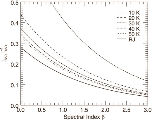
Effect of temperature on the emissivity spectral index β. For a given temperature, the theoretical ratio of flux densities (I850|$I_{450}^{-1}$|) is plotted as a function of the spectral index, as defined from equation (2), for an ideal case where there is no molecular contamination (Cλ = 0 ∀ λ). The solid line represents the temperature-independent case, obtained with the Rayleigh–Jeans approximation for dust thermal emission.
In order to evaluate the effect of molecular contamination on the spectral index of emissivity, we postulate that the fraction C850 from equation (3) comes entirely from 12CO J = 3−2 rotational line emission. We use a molecular emission map converted from HARP spectroscopic data using the technique presented by Drabek et al. (2012). It is important to note that this conversion depends on the effective transmission of the telescope, and therefore varies with the atmospheric conditions during the observations. Although it is not expected to be the only contributing factor, this 12CO J = 3−2 molecular line is the most likely culprit of molecular contamination at 850 μm as it is the brightest and most common emission line over the entire region except in OMC 1's bright core. Away from hot cores, the 12CO J = 3–2 line can be 5–10 times brighter in the 850 μm band than all other molecular lines combined (see Johnstone et al. 2003).
Similarly, we would expect the main driver of molecular contamination at 450 μm to be the emission from the 12CO J = 6−5 rotational line. Drabek et al. (2012) extrapolated from 12CO J = 3−2 observations that the molecular contamination C450 is, in most cases, unlikely to be significant when compared to the dust thermal emission at this wavelength. This can be verified in OMC 1 using the 12CO J = 6−5 integrated main-beam brightness temperature map from Peng et al. (2012). With the conversions factors from Drabek et al. (2012), it is possible to estimate the 12CO J = 6−5 contamination towards some key regions in our 450 μm observations: Orion KL, Orion South and the Orion bar. We estimate the contamination to be <1 per cent, <1 per cent and <5 per cent of the total 450 μm flux density for these regions, respectively. These estimates are likely to be upper limits since they do not take into account instrumental differences, such as sensitivity to large-scale emission, between CHAMP+ (Peng et al. 2012), HARP and SCUBA-2. It is therefore reasonable, at least for OMC 1, to assume the 12CO J = 6−5 line contamination to be negligible for SCUBA-2 observations at 450 μm. Since other molecular lines in that observation band are generally much weaker than the 12CO J = 6−5 line, except for hot cores (Peng et al. 2012), we limit this study only to the effects of contamination in the 850 μm band. The coefficient C850 can only decrease the 850–450 μm flux ratio, therefore the spectral index of emissivity will be underestimated if contamination from molecular emission is not taken into account. This may be particularly important in regions of strong molecular emission relative to the dust continuum, such as a low dust column-density region containing molecular outflows (Buckle et al. 2012).
3 OBSERVATIONS
The SCUBA-2 is a 10 000 pixel cryogenically cooled continuum camera capable of simultaneously observing in the 450 and 850 μm atmospheric windows (Holland et al. 2013). The HARP is a 16-element detector providing high-sensitivity and high-resolution spectral line measurements between 325 and 375 GHz (799 and 922 μm). The Auto-Correlation Spectral Imaging System is a digital interferometric spectrometer that can use HARP measurements to create large-scale velocity maps (Buckle et al. 2009).
Shared-risk observations of the Orion A molecular cloud complex were taken on 2010 February 13 at the JCMT with SCUBA-2. The measured 225 GHz atmospheric opacity during the observations varied between τ225 = 0.036–0.045. The complementary spectroscopic observations of the 12CO J = 3−2 molecular line were obtained between 2007 February 9 and 16 with HARP (Graves 2011). The opacity varied between τ225 = 0.079–0.094. The three maps cover a field of approximately 60 arcmin×60 arcmin. They include most of the Orion A molecular clouds along the integral-shaped filament, such as OMC 1 to OMC 3, as well as OMC 4 and the northernmost part of OMC 5.
The 12CO J = 3−2 emission line map used in this study was reduced independently from the SCUBA-2 shared-risk observations (Graves 2011). The Orion A shared-risk observations were reduced using the starlink software map-making capabilities (Chapin et al. 2010, 2015). The shared-risk programme for SCUBA-2 was completed with only one array (instead of the final four) of the detector in each continuum band, leading to less sensitive maps than what can be produced by the full detector (e.g. Salji et al. 2015; Mairs et al., in preparation). Because of differences in the way large-scale emission is handled between the shared-risk and the full-array reductions, the 12CO J = 3−2 contamination analysis presented in this study applies only to small-scale structures (<1 arcmin). Contamination levels for individual sources may change when larger spatial scales are included.
As mentioned in Section 2, some calibration is needed before the SCUBA-2 and HARP maps can be used together. Because of the way the telescope's dish distributes the incident energy over the detectors, the effective beam shape for each SCUBA-2 bandpass is approximated by two Gaussian components. The full width at half-maximum (FHWM) of these main and secondary beams are, respectively, 7.9 arcsec and 25 arcsec at 450 μm with relative amplitudes of 0.94 and 0.06. At 850 μm, they are 13.0 arcsec and 48 arcsec with relative amplitudes of 0.98 and 0.02 (Di Francesco et al. 2008; Dempsey et al. 2013). The process of beam-matching consists of convolving each map with the other's effective beam. This is done to ensure that the 450 and 850 μm maps are comparable by degrading their quality in similar ways. The 12CO J = 3−2 emission map is treated slightly differently. The map is first filtered with a Gaussian (FWHM = 1.0 arcmin) in order to subtract excess large-scale background (Drabek et al. 2012). This is made necessary by HARP's sensitivity to larger spatial scales than the 850 μm shared-risk observations. This large-scale emission can represent a significant proportion of the 12CO J = 3−2 integrated intensity (≈85 per cent in some parts of the cloud). It is then convolved with the 450 μm primary and secondary beams to degrade it in a similar way to the 850 μm map. This was done to treat CO data in a manner as close as possible to the 850 μm data. Once the beam-matching process is complete, an automated linear interpolation transforms the 450 μm and 12CO J = 3−2 maps to share the same pixel-scale (4.0 arcsec) and associated celestial coordinates as the 850 μm map.
Before the three maps can be used with equation (3), they first need to be properly normalized. Since we are working with peak photometry (Jy beam−1) instead of aperture photometry (Jy arcsec−2), this calibration must be included in the beam-matching process. We use the effective beam widths θE450 = 9.8 arcsec and θE850 = 14.6 arcsec from Dempsey et al. (2013) to calculate the new effective mixed beam width θM = 17.6 arcsec created by convolving the 450 and 850 μm beams together. After applying the appropriate filtering, each map is multiplied by a correction factor calculated from these effective beams to compensate for the change in beam area. Once this normalization is complete, the three maps effectively share the same units and can be directly compared.
The noise levels were calculated after the beam matching process, for an effective 17.6 arcsec beam width, by measuring the standard deviation of the background emission in each map. This was done by selecting a 276 arcsec × 172 arcsec low-emission region centred at (5:34:19.550, −5:42:41.91). To calculate the spectral index map, only pixels with a flux density above 1σ were used, which is 280 mJy beam−1 at 450 μm and 20 mJy beam−1 at 850 μm.
4 RESULTS
The shared-risk observations for Orion A are shown in Fig. 2 for the 850 and 450 μm bands. The measured 12CO J = 3−2 integrated intensity for a value of 20 K km s−1 is shown as the blue contour in the left-hand panel of Fig. 2. This figure also shows the emissivity spectral index α map from equation (3) after the 12CO J = 3−2 contamination was removed from the 850 μm map. An estimate of the regional variations in emissivity can be obtained from equation (5) in the Rayleigh–Jeans approximation: βRJ = α − 2. As stated previously, this approximation generally leads to an incomplete representation of low-temperature regions by underestimating the value of the spectral index β. However, it still shows some key features such as the low emissivity region in OMC 1 north-west of the Trapezium stars. This is a region with well-known contamination from molecular lines other than the 12CO J = 3−2 line (Groesbeck 1995; Serabyn & Weisstein 1995; Wiseman & Ho 1998). The Orion bar also shows low spectral index regions similar to those measured in previous studies (Lis et al. 1998; Johnstone & Bally 1999).
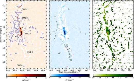
The Orion A molecular cloud complex as seen by the SCUBA-2 shared-risk observations. Left: continuum map at 850 μm in Jy per unit of 850 μm beam area. The blue contour traces the 20 K km s−1 emission from the 12CO J = 3−2 molecular line. The labels identify the approximate location of different regions in the integral-shaped filament. Middle: continuum map at 450 μm map in Jy per unit of 450 μm beam area. The 60 submillimetre sources selected for this study (see Tables 1 and 2) are identified as follows: clumps are black plus symbols, protostars are red triangles and young stars with discs are green diamonds. Right: map of the spectral index α as defined in equation (3). Its relationship to the spectral index of emissivity β is given in equation (5). In the Rayleigh–Jeans approximation, this relation is simplified to βRJ = α − 2. The red star identifies the position of θ Orionis C, the brightest member of the Trapezium cluster.
The 12CO J = 3−2 molecular line contamination is shown in Fig. 3 overlaid on the 850 μm continuum map. The green contours trace three levels of the 12CO J = 3−2 line emission as a percentage of the corresponding 850 μm flux density (10 per cent, 20 per cent and 30 per cent). To study molecular contamination in more detail, we chose 33 sources around the integral-shaped filament selected by eye for their higher level of 12CO J = 3−2 line emission. This represents most sources with a contamination C850 ≥ 0.1 in equation (3). Each area of high contamination is clearly labelled in Fig. 3. The continuum properties of these sources were checked individually to verify their plausibility as clump candidates. We took care to select sources away from possibly problematic regions in the 450 and 850 μm maps. This is made necessary because the contrast between intensities in the SCUBA-2 maps can create bowling effects that artificially decrease the flux density around very bright regions (OMC 1, for example). We also use 27 clumps identified by Johnstone & Bally (2006) in OMC 4. As these authors suspected, we confirm that these clumps have very low levels of 12CO J = 3−2 contamination and thus can be used as a control group.
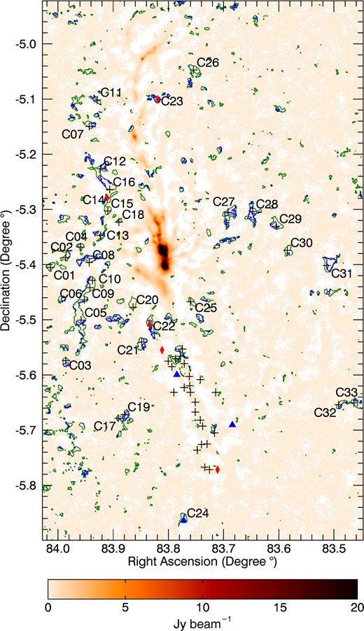
Continuum map of the Orion A molecular cloud complex at 850 μm in Jy per unit of 850 μm beam area. The contours trace two levels of the 12CO J = 3−2 molecular line contamination as a percentage of the corresponding 850 μm flux density (10 per cent in green and 30 per cent in blue). The 60 submillimetre sources selected for this study (see Tables 1 and 2) are identified as follows: clumps are black plus symbols, protostars are blue triangles and young stars with discs are red diamonds. For ease of reading, only the locations of high 12CO contamination (i.e., Table 1) are labelled.
The positions of all 60 sources are indicated in the 450 μm continuum map of Fig. 2, as well as in Fig. 3 (see caption). Their properties, shown in Tables 1 and 2, are obtained by averaging the values in each small 12 arcsec × 12 arcsec map box centred on the peak position of the source. These boxes have roughly the same angular area as the effective 850 μm beam. Table 1 lists the 33 sources selected for their higher levels of 12CO J = 3−2 molecular line contamination. Their IDs have been attributed in order of decreasing right ascension. Table 2 lists the 27 reference clumps in OMC 4. The ID for each clump is the same as given by Johnstone & Bally (2006).
Measured properties of 33 sources selected for their 12CO J = 3−2 contamination.
| ID | RAa | Dec.a | 〈S850〉b | σ850b | per centc | σ per centc | Ratiod | σRd | αe | 〈σα〉e | Δαf | YSOg |
|---|---|---|---|---|---|---|---|---|---|---|---|---|
| C01 | 05 36 03.24 | −05 24 18.0 | 108 | 16 | 15 | 3 | 0.11 | 0.04 | 3.5 | 0.6 | 0.3 | |
| C02 | 05 35 56.54 | −05 23 14.0 | 101 | 16 | 15 | 3 | 0.10 | 0.04 | 3.7 | 0.6 | 0.2 | |
| C03 | 05 35 56.55 | −05 34 26.0 | 145 | 16 | 20 | 3 | 0.17 | 0.06 | 2.8 | 0.6 | 0.4 | |
| C04 | 05 35 50.11 | −05 22 06.0 | 147 | 15 | 14 | 2 | 0.09 | 0.02 | 3.7 | 0.4 | 0.2 | |
| C05 | 05 35 49.85 | −05 30 02.0 | 180 | 16 | 19 | 2 | 0.11 | 0.03 | 3.4 | 0.4 | 0.3 | |
| C06 | 05 35 48.51 | −05 27 50.0 | 160 | 18 | 17 | 3 | 0.09 | 0.02 | 3.9 | 0.4 | 0.3 | |
| C07 | 05 35 46.35 | −05 08 58.0 | 70 | 18 | 14 | 5 | 0.11 | 0.07 | 3.5 | 1.1 | 0.2 | |
| C08 | 05 35 46.36 | −05 23 46.0 | 176 | 18 | 11 | 2 | 0.09 | 0.02 | 3.8 | 0.4 | 0.2 | |
| C09 | 05 35 46.10 | −05 26 30.0 | 265 | 17 | 14 | 1 | 0.10 | 0.02 | 3.6 | 0.3 | 0.2 | |
| C10 | 05 35 45.02 | −05 25 42.0 | 280 | 17 | 13 | 1 | 0.12 | 0.02 | 3.3 | 0.3 | 0.2 | |
| C11 | 05 35 42.87 | −05 06 06.0 | 131 | 18 | 8 | 2 | 0.09 | 0.03 | 3.8 | 0.4 | 0.1 | |
| C12 | 05 35 41.53 | −05 13 34.0 | 96 | 16 | 19 | 4 | 0.08 | 0.03 | 4.0 | 0.6 | 0.3 | |
| C13 | 05 35 41.54 | −05 20 50.0 | 63 | 7 | 15 | 2 | 0.08 | 0.02 | 3.9 | 0.4 | 0.3 | |
| C14 | 05 35 38.59 | −05 16 46.1 | 85 | 14 | 15 | 3 | 0.07 | 0.02 | 4.2 | 0.5 | 0.2 | YSD |
| C15 | 05 35 38.32 | −05 18 10.1 | 161 | 15 | 19 | 2 | 0.11 | 0.03 | 3.5 | 0.4 | 0.3 | |
| C16 | 05 35 37.52 | −05 15 50.1 | 159 | 14 | 11 | 2 | 0.09 | 0.02 | 3.8 | 0.3 | 0.2 | |
| C17 | 05 35 33.78 | −05 40 42.0 | 83 | 17 | 20 | 5 | 0.11 | 0.06 | 3.5 | 0.9 | 0.4 | |
| C18 | 05 35 33.50 | −05 19 22.1 | 197 | 17 | 11 | 2 | 0.18 | 0.05 | 2.7 | 0.5 | 0.2 | |
| C19 | 05 35 31.10 | −05 40 18.1 | 80 | 21 | 14 | 5 | 0.05 | 0.03 | 4.6 | 0.7 | 0.2 | |
| C20 | 05 35 27.35 | −05 28 38.1 | 93 | 15 | 17 | 4 | 0.08 | 0.03 | 4.0 | 0.5 | 0.3 | |
| C21 | 05 35 23.60 | −05 32 26.1 | 109 | 16 | 18 | 3 | 0.08 | 0.03 | 4.0 | 0.5 | 0.3 | |
| C22 | 05 35 20.11 | −05 30 30.1 | 40 | 13 | 16 | 6 | 0.06 | 0.04 | 4.4 | 1.0 | 0.3 | YSD |
| C23 | 05 35 16.63 | −05 06 02.1 | 155 | 17 | 44 | 5 | 0.08 | 0.03 | 3.9 | 0.6 | 0.9 | YSD |
| C24 | 05 35 05.37 | −05 51 50.0 | 154 | 16 | 16 | 2 | 0.16 | 0.05 | 2.9 | 0.5 | 0.3 | P |
| C25 | 05 35 02.43 | −05 28 02.1 | 129 | 15 | 12 | 2 | 0.17 | 0.06 | 2.8 | 0.6 | 0.2 | |
| C26 | 05 35 01.10 | −05 02 50.1 | 37 | 13 | 16 | 7 | 0.07 | 0.04 | 4.3 | 1.1 | 0.3 | |
| C27 | 05 34 46.10 | −05 18 18.0 | 83 | 18 | 23 | 6 | 0.08 | 0.04 | 4.0 | 0.8 | 0.4 | |
| C28 | 05 34 35.39 | −05 18 14.0 | 99 | 18 | 17 | 4 | 0.08 | 0.03 | 3.9 | 0.6 | 0.3 | |
| C29 | 05 34 25.21 | −05 19 50.0 | 71 | 15 | 31 | 8 | 0.06 | 0.03 | 4.3 | 0.8 | 0.6 | |
| C30 | 05 34 20.38 | −05 22 25.9 | 145 | 16 | 23 | 3 | 0.12 | 0.04 | 3.3 | 0.5 | 0.4 | |
| C31 | 05 34 03.24 | −05 24 05.8 | 151 | 15 | 21 | 3 | 0.08 | 0.02 | 3.9 | 0.4 | 0.4 | |
| C32 | 05 33 58.12 | −05 39 13.8 | 123 | 18 | 12 | 3 | 0.11 | 0.04 | 3.4 | 0.6 | 0.2 | |
| C33 | 05 33 51.42 | −05 39 01.7 | 91 | 17 | 13 | 3 | 0.13 | 0.06 | 3.2 | 0.8 | 0.2 |
a Right ascension and declination of the sources for epoch J2000.0.
b Average flux density and uncertainty (in mJy) per unit of effective 850 μm beam area (beam width of 14.6 arcsec).
c12CO J = 3−2 molecular emission and uncertainty as a percentage of the 850 μm flux density.
d Ratio of 850–450 μm flux densities corrected for 12CO J = 3−2 contamination and uncertainty.
e Spectral index corrected for 12CO J = 3−2 contamination as shown in equation (3) and average uncertainty.
f Spectral index difference after correction for 12CO J = 3−2 line emission.
g Young stellar object: protostar (P) or young star with disc (YSD).
Measured properties of 27 clumps identified in OMC 4 by Johnstone & Bally (2006).
| ID | RAa | Dec.a | 〈S850〉b | σ850b | per centc | σ per centc | Ratiod | σRd | αe | 〈σα〉e | Δαf | YSOg |
|---|---|---|---|---|---|---|---|---|---|---|---|---|
| 01 | 05 34 44.21 | −05 41 26.0 | 258 | 18 | 0 | 1 | 0.14 | 0.03 | 3.1 | 0.3 | 0.0 | P |
| 02 | 05 34 50.63 | −05 46 18.0 | 105 | 14 | 2 | 2 | 0.07 | 0.02 | 4.1 | 0.4 | 0.0 | YSD |
| 03 | 05 34 51.44 | −05 37 54.0 | 57 | 16 | 0 | 3 | 0.12 | 0.08 | 3.3 | 1.1 | 0.0 | |
| 04 | 05 34 51.98 | −05 42 18.0 | 69 | 20 | 1 | 3 | 0.07 | 0.03 | 4.3 | 0.7 | 0.0 | |
| 05 | 05 34 54.12 | −05 46 18.0 | 438 | 15 | 0 | 1 | 0.14 | 0.02 | 3.0 | 0.2 | 0.0 | |
| 06 | 05 34 55.19 | −05 43 30.0 | 135 | 16 | 0 | 1 | 0.06 | 0.02 | 4.3 | 0.3 | 0.0 | |
| 07 | 05 34 56.26 | −05 46 02.0 | 634 | 15 | 0 | 1 | 0.14 | 0.01 | 3.1 | 0.1 | 0.0 | |
| 08 | 05 34 57.07 | −05 41 34.1 | 224 | 16 | 0 | 1 | 0.08 | 0.01 | 3.9 | 0.2 | 0.0 | |
| 09 | 05 34 57.60 | −05 43 34.0 | 48 | 29 | 1 | 5 | 0.02 | 0.02 | 6.2 | 1.3 | 0.0 | |
| 10 | 05 34 58.14 | −05 36 30.1 | 78 | 17 | 0 | 2 | 0.08 | 0.03 | 4.0 | 0.6 | 0.0 | |
| 11 | 05 34 58.14 | −05 40 54.1 | 173 | 16 | 0 | 1 | 0.09 | 0.02 | 3.8 | 0.3 | 0.0 | |
| 12 | 05 34 59.48 | −05 44 10.1 | 109 | 19 | 0 | 2 | 0.11 | 0.04 | 3.5 | 0.6 | 0.0 | |
| 13 | 05 35 00.29 | −05 38 58.1 | 311 | 16 | 0 | 1 | 0.12 | 0.02 | 3.3 | 0.2 | 0.0 | |
| 14 | 05 35 00.29 | −05 40 02.1 | 210 | 19 | 0 | 1 | 0.10 | 0.02 | 3.6 | 0.3 | 0.0 | |
| 16 | 05 35 02.70 | −05 37 10.1 | 130 | 14 | 0 | 1 | 0.08 | 0.02 | 4.1 | 0.3 | 0.0 | |
| 17 | 05 35 02.43 | −05 37 54.1 | 264 | 17 | 0 | 1 | 0.09 | 0.01 | 3.8 | 0.2 | 0.0 | |
| 18 | 05 35 02.97 | −05 36 10.1 | 478 | 16 | 0 | 1 | 0.10 | 0.01 | 3.6 | 0.1 | 0.0 | |
| 19 | 05 35 05.11 | −05 37 22.1 | 513 | 17 | 0 | 1 | 0.11 | 0.01 | 3.5 | 0.1 | 0.0 | |
| 20 | 05 35 05.11 | −05 34 46.1 | 453 | 18 | 0 | 1 | 0.09 | 0.01 | 3.8 | 0.2 | 0.0 | |
| 21 | 05 35 05.91 | −05 33 10.1 | 336 | 18 | 4 | 1 | 0.10 | 0.02 | 3.6 | 0.2 | 0.1 | |
| 22 | 05 35 06.72 | −05 33 58.1 | 86 | 17 | 6 | 2 | 0.05 | 0.02 | 4.8 | 0.5 | 0.1 | |
| 24 | 05 35 08.33 | −05 35 58.1 | 835 | 18 | 0 | 1 | 0.12 | 0.01 | 3.3 | 0.1 | 0.0 | P |
| 28 | 05 35 08.86 | −05 34 14.1 | 65 | 22 | 8 | 4 | 0.04 | 0.02 | 5.3 | 0.8 | 0.1 | |
| 32 | 05 35 09.66 | −05 37 54.1 | 176 | 17 | 0 | 1 | 0.21 | 0.07 | 2.5 | 0.5 | 0.0 | |
| 34 | 05 35 10.47 | −05 35 06.1 | 466 | 17 | 0 | 1 | 0.11 | 0.01 | 3.5 | 0.2 | 0.0 | |
| 36 | 05 35 12.08 | −05 34 30.1 | 560 | 18 | 1 | 1 | 0.11 | 0.01 | 3.5 | 0.1 | 0.0 | |
| 39 | 05 35 14.76 | −05 33 18.1 | 144 | 19 | 0 | 1 | 0.16 | 0.06 | 2.9 | 0.6 | 0.0 | YSD |
a Right ascension and declination of the sources for epoch J2000.0.
b Average flux density and uncertainty (in mJy) per unit of effective 850 μm beam area (beam width of 14.6 arcsec).
c12CO J = 3−2 molecular emission and uncertainty as a percentage of the 850 μm flux density.
d Ratio of 850–450 μm flux densities corrected for 12CO J = 3−2 contamination and uncertainty.
e Spectral index corrected for 12CO J = 3−2 contamination as shown in equation (3) and average uncertainty.
f Spectral index difference after correction for 12CO J = 3−2 line emission.
g Young stellar object: protostar (P) or young star with disc (YSD).
The 12CO J = 3−2 contamination in each clump expressed as a percentage of their average 850 μm flux density is plotted versus their average 850 μm flux density per unit of effective 850 μm beam area (θE850 = 14.6 arcsec) in Fig. 4; the same contamination percentage is given in Fig. 5 as a function of the 850–450 μm flux ratio. Although we use the beam-matched (θM = 17.6 arcsec) values to calculate the contamination and the ratio of flux densities (and thus the spectral indices), it is more useful for future studies to describe the sources presented in this paper by their 〈S850〉 flux density per unit of effective 850 μm beam area. The 12CO J = 3−2 contamination as a percentage of the 850 μm flux density remains essentially unchanged between the matched (θM) and effective (θE850) beams.
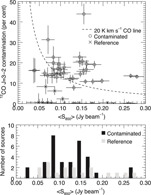
Top: 12CO J = 3−2 molecular line emission as a percentage (per cent) of the corresponding average flux density 〈S850〉 (Jy beam−1) measured directly from the SCUBA-2 850 μm shared-risk observation map. The dashed line sets the percentage of contamination for a 12CO J = 3−2 line emission at 20 K km s−1. The empty circles are the 33 sources chosen in this study for their high level of molecular contamination. The crosses are reference sources identified by Johnstone & Bally (2006) in OMC 4 with an average flux density lower than 0.3 Jy beam−1. Since no reference source above 0.3 Jy beam−1 shows significant contamination, the horizontal axis is truncated at that value to facilitate the viewing of this figure. The uncertainties for all sources are identified with plain black lines. Bottom: histogram showing the distribution of contaminated (black bars) and reference (grey bars) sources as a function of their average flux density 〈S850〉 (Jy beam−1). The categories have a width of 0.02 Jy beam−1, with a range going from 0.00 to 0.30 Jy beam−1.
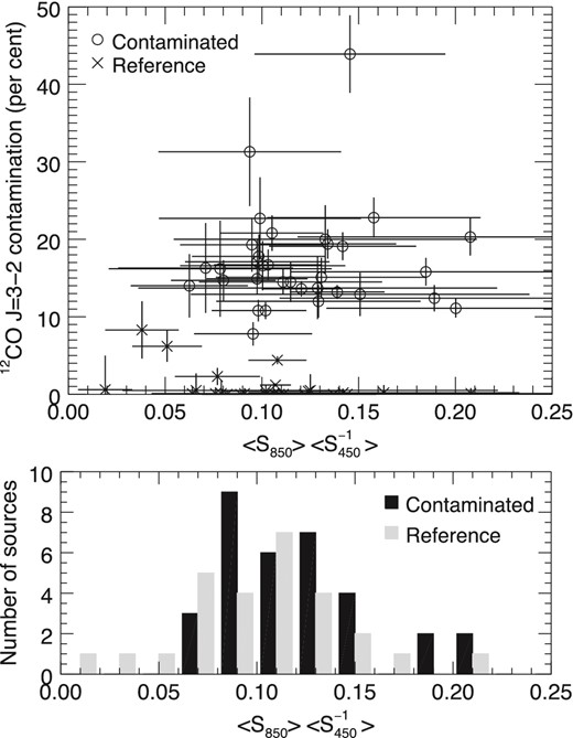
Top: 12CO J = 3−2 molecular line emission as a percentage ( per cent) of the corresponding average 850 μm flux density 〈S850〉, as a function of the measured (i.e., uncorrected for CO contamination) 850–450 μm average flux ratio 〈S850〉〈S450〉−1. The symbols have the same meaning as in Fig. 4. For each source, these two quantities are used in equation (3) to deduce the spectral index α before and after contamination correction. The uncertainties for all sources are identified with plain black lines. Bottom: histogram showing the distribution of contaminated (black bars) and reference (grey bars) sources as a function of their average flux ratio 〈S850〉〈S450〉−1. The histogram bins have a width of 0.02, with a range going from 0.00 to 0.26.
This list of 60 sources in Orion A was compared to a catalogue of known young stellar objects identified by Megeath et al. (2012) using the Spitzer Space Telescope. We confirm the presence of three protostars (blue triangles in Fig. 3) in our sample, including one (C24), showing a 12CO J = 3−2 contamination of 16 per cent, in the northernmost part of OMC 5. Furthermore, five young stars with discs lie within continuum sources along the integral-shaped filament, including three in regions with strong 12CO J = 3−2 line emission. The most highly contaminated source in this study (C23), with a level of 44 per cent, is associated with a young star with a disc located between OMC 2 and OMC 3 (identified in Fig. 3). It is unlikely that this object alone is responsible for such a strong 12CO J = 3−2 line emission. Some possible explanations include that this region is a shock knot, or that it is surrounded by outflows from past or ongoing star formation. The objects in our sample that have also been detected with the Spitzer Space Telescope are identified on Fig. 3 (see caption) and listed in Tables 1 and 2. Additional notes on astronomical objects found near these sources of interest are presented in Appendix B.
To check for signs of molecular outflows, the wing criterion from Hatchell, Fuller & Richer (2007) (TMB > 1.5 K at 3.0 km s−1 from line centre) was applied to the spectrum of each source from Tables 1 and 2. This criterion is reached for most sources in both the contaminated and reference samples; the spectra often exhibit wide 12CO J = 3−2 molecular lines. The wing criterion is not met in only a few cases: five sources in the contaminated sample (C12, C17, C19, C32, C33) and one in the reference sample (06). All the Spitzer-identified young stellar objects listed in Tables 1 and 2 also fit the wing criterion with wide 12CO J = 3−2 lines. It is therefore likely that molecular outflows play a major role in 12CO J = 3−2 line contamination at 850 μm.
Before we study the effect of molecular line contamination in more detail, we can deduce some general guidelines concerning 12CO J = 3−2 emission in the sources shown on Fig. 4. First of all, all the identified sources with a contamination level above 10 per cent seem to be concentrated below a threshold of 300 mJy beam−1 in the 850 μm SCUBA-2 shared-risk map. Such a limit is to be expected because the optically thick 12CO J = 3−2 line emission saturates much faster than the mostly optically thin dust thermal emission. The 12CO J = 3−2 line emission is therefore more likely to become a problem towards regions of lower column density. This also explains why peaks in 12CO J = 3−2 line emission do not necessarily lead to high levels of contamination in SCUBA-2 maps. The OMC 1 central 12CO J = 3−2 emission peak is an example of this situation; it is completely dominated by the total 850 μm peak flux density: it produces a contamination ≤1 per cent. This does not mean that the total molecular contamination in the central part of OMC 1 is negligible; it is a region known for its multitude of molecular species (Serabyn & Weisstein 1995; Wiseman & Ho 1998) which may contribute up to 60 per cent of its 850 μm intensity (Groesbeck 1995). There is however no easy way to guess which sources will be contaminated by molecular emission without having the corresponding spectroscopic observations. Even among sources with the same classification, as we see in Spitzer-identified protostars and young stars with discs in our sample, there can be wide differences in the levels of 12CO J = 3−2 line emission. The sources that do show a strong molecular contamination must be corrected as their deduced physical properties depend on an accurate measurement of flux density.
The most direct effect of 12CO J = 3−2 molecular line emission is its contribution to the total 850 μm flux density measured by SCUBA-2, therefore inflating the resulting 850–450 μm flux ratio. Following equation (3) and Fig. 1, this systematically leads to an underestimation of the spectral indices α and β. The size of this deviation depends on the fraction of molecular line contamination in the measured 850 μm flux density, as shown in equation (4). The percentage of 12CO J = 3−2 molecular line emission and the measured 850–450 μm flux ratios are shown in Fig. 5 for a sample of 60 sources in Orion A. The largest spectral index difference (|$\Delta \alpha =0.9^{+0.3}_{-0.1}$|) is associated with an object (C23) with a 12CO J = 3−2 line contamination percentage of 44 per cent. Its average 850–450 μm flux ratio is reduced from 0.15 ± 0.04 to 0.08 ± 0.03, thus increasing the deduced spectral index α from |$3.0^{+0.5}_{-0.4}$| to |$3.9^{+0.6}_{-0.4}$|.
The effects of molecular contamination on emissivity can also be understood by looking at the histograms in Fig. 6. By using the flux ratio as a proxy for the spectral index β, following the same relation as the one shown in Fig. 1, we directly quantify the difference 12CO J = 3−2 line subtraction has on the emissivity of both the total source selection and the contaminated subgroup. The top panel of Fig. 6 quantifies how correcting the 850 μm flux density influences the 850–450 μm flux ratio for the 33 most highly contaminated sources in our sample. By combining equation (3) with the measurements shown in Fig. 5, we calculate the spectral index α before and after contamination correction for all 60 sources. The results are presented in Tables 1 and 2. The average uncorrected ratio of these sources leads to a spectral index |$\left\langle \alpha \right\rangle = 3.3^{+0.6}_{-0.4}$|. The corresponding average correction is |$\left\langle \Delta \alpha \right\rangle = 0.3^{+0.2}_{-0.2}$|. This results in an average corrected value |$\left\langle \alpha \right\rangle = 3.6^{+0.6}_{-0.4}$| for the contaminated sources. In comparison, the spectral index for the OMC 4 control group gives a value |$\left\langle \alpha _{{\rm O\!M\!C}4}\right\rangle = 3.6^{+0.8}_{-0.5}$|. The uncertainties are obtained from the standard deviations of the ratios. Although they are statistical uncertainties, we have just enough sources in each sample (33 and 27) for them to be significant. If these two samples are indeed comparable, as their similar standard deviations and their distribution of ratios in Fig. 5 would suggest, then this indicates that the contamination correction brings the average spectral indices α to levels similar to those in the uncontaminated clumps of OMC 4. The similarity between the two samples could be explained by the selection of sources away from the ridge in OMC 1 (see Fig. 2), known to be warmer and denser than the rest of the integral shaped filament.
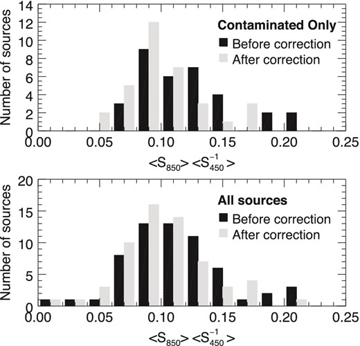
Histograms showing the effect of contamination correction on the 850–450 μm average flux ratio 〈S850〉〈S450〉−1. The number of sources for each bin is given before (black bars) and after (grey bars) contamination correction is applied to the measured ratio. The histogram bins have a width of 0.02, with a range going from 0.00 to 0.26. Top: the histogram is limited to the 33 sources chosen in this study for their high level of molecular contamination. Bottom: the histogram including all 60 sources shown in Fig. 5.
A Kolmogorov–Smirnov test was applied to both the contaminated and the total subgroups from Fig. 6 in order to verify the significance of the contamination correction on these distributions. The subgroup with the 33 contaminated sources has a 0.8 per cent probability that the uncorrected and corrected distributions are statistically identical. Since it represents the group most affected by molecular contamination, this is a confirmation that contamination correction has a significant effect on the measured flux ratios. For the complete selection, this test gives a 6.4 per cent probability. Unsurprisingly, this only means that, as more uncontaminated sources are added to the sample tested, the less statistically significant the average contamination becomes.
5 DISCUSSION
Quantifying the molecular line contamination in submillimetre observations, such as in SCUBA-2 850 μm maps, is a necessary step in the study of cold interstellar dust. Through the construction of accurate spectral energy distributions, it is possible to learn much about the physical properties of this important mass tracer in giant molecular clouds. As an example, models using observations carried out with the Herschel Space Observatory, hereafter Herschel, benefit strongly from the addition of SCUBA-2 850 μm measurements. While Herschel observations efficiently probe the peak blackbody emission of cold dust grains, SCUBA-2 wavelengths help constrain the Rayleigh–Jeans tail of the distribution. This leads to a better determination of density, temperature and spectral index β than Herschel results alone (Sadavoy et al. 2013). Furthermore, both the JCMT and Herschel have significant overlapping data in the Gould Belt.
A good example of what can be achieved with a multifaceted approach is the work of Lombardi et al. (2014). These authors combined observations from the Planck and Herschel space telescopes in order to build optical depth and temperature maps for the Orion molecular cloud complex. They also included in their fits the spectral index β map from Planck Collaboration XIX (2011) at a resolution of 36 arcmin. From this optical depth map, and with near-infrared extinction measurements from 2MASS, Lombardi et al. (2014) obtained a column density map for the region. Finally, they found a temperature Td ≈ 15 K in dense regions along the spine of Orion A, which we will use as a reference for the examples used in this discussion.
Since dust thermal emission depends strongly on the emissivity of the grains, we focus specifically on how molecular contamination influences this property. This is why we use the spectral index β instead of α for the rest of this discussion. We have already given in Section 2 a relation between the spectral indices α and βRJ obtained from equation (5) in the Rayleigh–Jeans approximation: βRJ = α − 2. This allows us to use these indices interchangeably to calculate differences (Δα = Δβ), assuming the dust temperature Td is fixed. The Rayleigh–Jeans approximation also provides us with a reliable lower limit for the more realistic emissivity spectral index β.
First, the results given in Section 4 need to be put into proper context. The dust in the diffuse interstellar medium is generally expected to have an emissivity spectral index near β = 1.7 (Weingartner & Draine 2001). This has been confirmed by the Planck Collaboration XI (2014) paper, where they measured a mean value of β = 1.62 ± 0.10 at high Galactic latitudes. In molecular clouds and their dense filaments, the emissivity is however usually assumed constant at β = 2.0 (Arzoumanian et al. 2011; Palmeirim et al. 2013; Salji et al. 2015). The spectral index in collapsing cores can vary between β = 1.7–2.0, while in protostellar discs, it drops quickly below β ≤ 1.7 as the grain sizes increase (Natta et al. 2007). The emissivity can also change depending on the region studied. As an example, there is strong evidence of larger dust grains decreasing the emissivity in some pre-stellar cores of OMC 2 and OMC 3 (Schnee et al. 2014). The presence of ice mantles on dust grains can also, in theory, play a crucial role for the emissivity as they tend to increase the spectral index β (Ossenkopf & Henning 1994; Shirley et al. 2005).
From this perspective alone, the average Rayleigh–Jeans emissivity spectral index βRJ obtained in Section 4 after correction for 12CO J = 3−2 contamination (|$\left\langle \beta _{{\rm RJ}} \right\rangle = 1.6^{+0.6}_{-0.4}$|) could be interpreted as at the lower limit for cores and filaments. While our spectral index map in Fig. 2 is very similar to the one presented by Johnstone & Bally (1999), the mean corrected indices for the contaminated and control samples (βRJ ≈ 1.6) are in fact slightly higher than expected from using the temperature-independent Rayleigh–Jeans approximation. Even if this approximation is useful to establish lower limits, we showed in Fig. 1 that it underestimates the spectral index towards cold regions. As an example, a pre-stellar core with a real emissivity spectral index β = 2.0 at a temperature Td = 15 K would have, using equation (5), an associated spectral index α = 3.0 (βRJ = 1.0). This illustrates the importance of knowing the temperature for finding a reliable value of the emissivity spectral index β.
A possible explanation for the statistical uncertainties in the average measured Rayleigh–Jeans emissivity spectral index |$\left\langle \beta _{{\rm RJ}} \right\rangle = 1.6^{+0.6}_{-0.4}$| is that we are comparing objects of different natures. Since the properties of most sources in our sample are unknown, they could very well cover a large intrinsic range of emissivity spectral indices β as well as dust temperatures Td. This spread of measured spectral indices could also be explained in part by the uncertainties on the measured ratios, as they are shown in Fig. 5. Since the ratio method presented in this work is sensitive to small flux variations, these uncertainties are mostly driven by the noise level in the 450 μm flux density map. Furthermore, if the 450 μm map is more susceptible to large-scale fluctuations than its 850 μm counterpart, it could contribute to the artificial decrease in the measured ratios, thus increasing the average measured spectral indices for each sample. Although this leads to a large range of values for the Rayleigh–Jeans emissivity spectral index βRJ, we know from equations (4) and (5) that the correction Δβ for each source depends on the more accurate HARP measurements and on the smoother 850 μm map. We are confident that this measured effect of molecular contamination on the emissivity spectral index β is a reliable estimate, even if the spectral indices themselves are subject to large uncertainties and probably also intrinsic spread.
The variation in the average spectral index due to 12CO J = 3−2 line contamination correction |$\left\langle \Delta \beta \right\rangle = 0.3^{+0.2}_{-0.2}$| illustrates the different scenarios possible in sources contaminated by molecular line emission. For some, it only acts as a correction leading to a slightly more accurate emissivity spectral index β. There are however cases where the difference is dramatic enough to change the physical description of the dust mixture in a submillimetre source. As an example, the most highly contaminated source in the sample (C23, 44 per cent), associated with a Spitzer-identified young star with disc, gives a large correction |$\Delta \beta =0.9_{-0.1}^{+0.3}$| that brings it on par with the average Rayleigh–Jeans spectral index measured in OMC 4 (βRJ ≈ 1.6). This Δβ ≈ 0.9 could mean the difference between grain growth up to centimetre sizes typical of protostellar discs (β < 1.0), and the emissivity spectral index expected in collapsing cores (β > 1.7; Natta et al. 2007). The other contaminated Spitzer objects (C14, C22, C24, 16 ± 1 per cent) all share a correction Δβ ≈ 0.3 comparable to the average difference 〈Δβ〉 obtained from the entire contaminated sample. As discussed in the previous section, objects of these types (protostars and young stars with discs) are likely to be associated with molecular outflows, which would explain their 12CO J = 3−2 line contamination levels (Hatchell et al. 2007).
The dust temperature Td was assumed fixed up to this point for the analysis of the sources presented in this paper. If we instead suppose a fixed emissivity spectral index β = 2.0 (Hatchell et al. 2013; Rumble et al. 2015; Salji et al. 2015), it is possible to rewrite equations (4) and (5) to evaluate numerically the effect of molecular line contamination on the temperature determination (ΔTd). For the previous example of a theoretical submillimetre source with an emissivity spectral index β = 2.0 and a temperature Td = 15 K, a contamination level of ≈15 per cent (Δα = 0.3) would then lead to a measured temperature T = 12 K. This temperature determination is however sensitive to the slightest variation in the 850–450 μm flux ratio. It becomes unreliable as the temperature increases and the thermal emission approaches the Rayleigh–Jeans regime.
While the 850–450 μm flux ratio method is relevant to evaluate the effects of molecular contamination on the emissivity spectral index β, it is insufficient to properly derive the physical properties of cold interstellar dust grains. It requires some prior assumptions about the emissivity or the temperature, and it is insensitive to line-of-sight density variations (Shetty et al. 2009b). A more accurate determination of those properties requires a multiwavelength approach (Schnee et al. 2010; Arab et al. 2012). Even then, molecular line contamination can remain a concern in spectral energy distributions built using SCUBA-2 850 μm observations. As an example, the dust temperature Td in cold interstellar regions can be well constrained by fitting the peak thermal emission with Herschel observations alone. On the other hand, the determination of the emissivity spectral index β benefits from the addition of accurate SCUBA-2 850 μm measurements. In their study of the B1 clump in the Perseus molecular cloud, Sadavoy et al. (2013) showed that combining observations from both Herschel and SCUBA-2 lead to a better fit than using the Herschel data alone for the spectral energy distribution.
The degeneracy between the spectral index β and the temperature Td is a serious challenge when attempting to fit accurate spectral energy distributions. Shetty et al. (2009a) have shown that noise from observations can induce an artificial anti-correlation between β and Td when using a χ2 fitting method. This is confirmed by Kelly et al. (2012), who then introduced a hierarchical Bayesian fitting technique as an alternative to the χ2 method. The hierarchical Bayesian technique recovers the parameters of an artificial distribution with more accuracy; it is less sensitive to statistical noise and calibration uncertainties. It has also been successfully tested on Herschel observations of CB244. Furthermore, Juvela et al. (2013) compared several fitting methods and found they all exhibited some level of bias when estimating the relationship between β and Td. In particular, the hierarchical Bayesian model presented in Kelly et al. (2012), while more precise than the χ2 method, is nonetheless biased towards a flat β(Td) relation in sources with a low signal-to-noise ratio.
It is important to point out other possible sources of contamination in the SCUBA-2 observations. Although generally much fainter than 12CO lines, the contribution from other molecular lines, such as those from 13CO and C18O (Goldsmith, Bergin & Lis 1997; Buckle et al. 2012; Peng et al. 2012), can add up to a significant portion of the total flux at both 450 and 850 μm towards hot cores. The Orion KL hot core in OMC 1 is famous for having a forest of molecular lines (Serabyn & Weisstein 1995; Wiseman & Ho 1998) contributing a significant fraction (≈60 per cent) of its total flux density at 850 μm (Groesbeck 1995). This is also true at 450 μm, where the corresponding molecular lines contribute up to ≈15 per cent of the total flux density towards Orion KL (Schilke et al. 2001).
Another common source of contamination is the continuum free–free emission from electrons in the interstellar medium. While it generally represents only a small fraction (≤1 per cent) of the submillimetre emission at 850 μm in the Galactic Plane (Planck Collaboration XXIII 2014), it can become non-negligible towards regions with strong photo-ionization. As an example, free–free emission in extended H ii optically thin regions typically follow a gentle, almost flat, power law (Oster 1961; Mezger & Henderson 1967). It is therefore likely to be measurable even at submillimetre wavelengths. However, this is not necessarily true for partially thick jets or stellar winds where the free–free spectrum can be steeper (Reynolds 1986). In those cases, the contamination will depend on the properties of the observed object. One such example is the MWC 297 Herbig B1.5 star in the Serpens molecular cloud, which exhibits free–free contamination of 73 per cent and 82 per cent at 450 and 850 μm, respectively (Rumble et al. 2015).
Several regions in the Orion A molecular cloud show a strong free–free continuum. Dicker et al. (2009) fitted the dust thermal emission and the free–free emission towards three locations in OMC 1. The highest free–free contamination they found at 850 μm (≈10 per cent) is towards the free–free emission peak near the Trapezium stars. For Orion KL and Orion South, the free–free emission has only a small contribution (≤5 per cent of the total flux density at 850 μm). In each case, the free–free component at 450 μm is negligible (<1 per cent) when compared to the dust thermal emission. Lis et al. (1998) also estimated free–free contamination in OMC 1 observations at 1110 μm. This contamination reaches up to 75 per cent in the H ii region south-east of the Trapezium stars, and ≈10 per cent in the Orion bar. If we use these results as upper limits for the free–free contamination at 850 μm, it is possible to estimate its effect on the spectral index β that would be calculated from SCUBA-2 observations. If free–free emission is negligible at 450 μm, we know from equation (4) that contamination levels of ≈75 per cent and ≈10 per cent at 850 μm would overestimate the spectral index by Δβ ≈ 2.2 and Δβ ≈ 0.2, respectively. However, considering the strong free–free emission towards the H ii region, it is possible given a flat power-law that this contribution is not negligible at 450 μm after all. If the 450 μm emission has some component of free–free emission, this would reduce the bias in the measurement of beta, but would not eliminate it completely.
6 CONCLUSION
We have presented the SCUBA-2 shared-risk observations for the Orion A molecular cloud complex at 450 and 850 μm. They were combined with HARP spectroscopic measurements in order to evaluate the effects of molecular contamination on the emissivity spectral index β. We studied a list of 33 sources along the integral-shaped filament chosen for their high 12CO J = 3−2 line emission. At least four young stellar objects identified with the Spitzer Space Telescope [three young stars with discs (C14, C22, C23) and one protostar (C24)] show significant levels of contamination in their measured 850 μm flux densities. From the analysis of these contaminated sources, we have concluded that 12CO J = 3−2 line contamination leads to an average underestimation |$\left\langle \Delta \beta \right\rangle = 0.3^{+0.2}_{-0.2}$| in affected sources, with some individual sources displaying larger differences (up to |$\Delta \beta =0.9_{-0.1}^{+0.3}$|). While there is no obvious continuum property to easily identify contaminated sources, these results illustrate the need to subtract 12CO J = 3−2 line emission from SCUBA-2 850 μm continuum maps where the corresponding HARP measurements are available. The properties shared by the contaminated sources seem to be their peak emission threshold (S850 ≤ 300 mJy beam−1) and their more likely location towards regions of low dust column density. Emissivity is a crucial parameter for the description of dust grains in the interstellar medium, as it is related directly to size distributions in dust mixtures. Measuring it accurately is a necessary step in order to reach, with far-infrared and submillimetre observations, a more complete understanding of the physical processes leading to the formation of stars and their planetary systems.
Special thanks to John Bally, Patrice Beaudoin, Jonathan Gagné, Maryvonne Gérin and Sarah Sadavoy for enlightening discussions. We would like to thank the referee for their suggestions, which helped improve the discussion presented in this paper. This study has been achieved thanks to the support of the staff at the Joint Astronomy Centre and the members of the JCMT Gould Belt Survey team. This work would not have been possible without the support of the National Sciences and Engineering Research Council of Canada. This research has made use of the SIMBAD data base, operated at CDS, Strasbourg, France.
See JCMT Gould Belt Survey membership list in Appendix A.
REFERENCES
APPENDIX A: THE JCMT GOULD BELT SURVEY TEAM
The full members of the JCMT Gould Belt Survey consortium (2015 July) are:
P. Bastien, D. S. Berry, D. Bresnahan, H. Broekhoven-Fiene, J. Buckle, H. Butner, M. Chen, A. Chrysostomou, S. Coudé, M. J. Currie, C. J. Davis, J. Di Francesco, E. Drabek-Maunder, A. Duarte-Cabral, M. Fich, J. Fiege, P. Friberg, R. Friesen, G. A. Fuller, S. Graves, J. Greaves, J. Gregson, J. Hatchell, M. R. Hogerheijde, W. Holland, T. Jenness, D. Johnstone, G. Joncas, H. Kirk, J. M. Kirk, L. B. G. Knee, S. Mairs, K. Marsh, B. C. Matthews, G. Moriarty-Schieven, J. C. Mottram, C. Mowat, K. Pattle, J. Rawlings, J. Richer, D. Robertson, E. Rosolowsky, D. Rumble, S. Sadavoy, C. Salji, H. Thomas, N. Tothill, S. Viti, D. Ward-Thompson, G. J. White, J. Wouterloot, J. Yates, and M. Zhu.
APPENDIX B: NOTES ON INDIVIDUAL SOURCES
Several sources listed in Tables 1 and 2 have also been linked to Spitzer-identified young stellar objects from the Megeath et al. (2012) catalogue. For completeness, this section lists known objects found in the SIMBAD data base within 14.6 arcsec of these SCUBA-2 submillimetre sources (Wenger et al. 2000). These associated objects are listed in roman numerals under each source presented in the following subsections.
B1 Contaminated sample
Even though the sources in the contaminated sample (see Table 1) were identified based on their strong 12CO J = 3−2 line contamination, there are young stars within one 850 μm effective beam-width (14.6 arcsec) of their central position. These are typical variable stars, some of them with significant reddening. There are also two Herbig–Haro emission jets in the surroundings of the contaminated sources.
B1.1 Source C14
V* V2560 Ori is an Orion-type variable star with a spectral type of M6 located 13.2 arcsec mostly south of C14 with V = 19.2 and K = 11.7;
2MASS J05353920−0516355 is an irregular-type variable star located 14.08 arcsec north-east of C14 with I = 17.4 and K = 11.4.
B1.2 Source C22
MGM2012 1539 is an irregular-type variable star with a spectral type of M5.5 located 4.2 arcsec north-west of C22 with V = 18.6 and K = 11.9;
V* V1514 Ori is an Orion-type variable star with a spectral type M4.5e located 8.9 arcsec south-west of C22 with V = 17.9 and K = 10.2;
V* MY Ori (Parenago 1963) is an Orion-type variable star with a spectral type M5e located 9.8 arcsec south-east of C22 with V = 16.2 and K = 10.2;
HH 561 is an Herbig–Haro object located 10.3 arcsec south-east of C22.
B1.3 Source C23
TKK 544 is an infrared source located 2.7 arcsec north-west of C23 with J = 13.3 and K = 11.1, and it is somewhat nebulous on the 2MASS image;
2MASS J05351649−0506003 (MGM2012 2363) is a pre-main-sequence star also located 2.7 arcsec north-west of C23 with J = 16.6 and K = 13.6;
JBV2003 SK1−OMC 3 is a submillimetre source identified with SCUBA by Johnstone et al. (2003) and whose peak is located 5.6 arcsec east of C23;
HH 357 is an Herbig–Haro object located 11.2 arcsec south-west of C23.
B1.4 Source C24
2MASS J05350553−0551540 is a young stellar object located 4.8 arcsec south-east of C24 with H = 16.0 and K = 13.9, and it has a nebulous ‘tail’ on the 2MASS image.
B2 Reference sample
The reference sample (see Table 2) consists of sumillimetre clumps found in OMC 4 and listed in Johnstone & Bally (2006). They were selected as a control group for the contaminated sample because of their low 12CO J = 3−2 line contamination in the 850 μm band.
B2.1 Source 01
ISOY J053444.05−054125.7 is a young stellar object located 2.2 arcsec west of source 01;
JCMTSF J053443.8−054126, a submillimetre source identified with SCUBA, is a young stellar object candidate listed in Di Francesco et al. (2008) and whose peak is located 6.1 arcsec west of source 01.
B2.2 Source 02
MGM2012 1216 is a pre-main-sequence star located 13.0 arcsec north-east of source 02;
JCMTSE J053449.8−054614 is a submillimetre source identified with SCUBA, listed in Di Francesco et al. (2008) and whose peak is located 13.0 arcsec mostly west of source 02.
B2.3 Source 24
MGM2012 1400 is a young stellar object located 3.1 arcsec of source 24;
JCMTSF J053507.9−053556, a submillimetre source identified with SCUBA, is a young stellar object candidate listed in Di Francesco et al. (2008) and whose peak is located 6.8 arcsec mostly west of source 24;
2MASS J05350800−0535537 is a star located 6.8 arcsec north-west of source 24 with I = 21.7 and K = 15.2.
B2.4 Source 39
V* V2260 Ori is an Orion-type variable star with a spectral type K4−M0 located 4.8 arcsec west of source 39 with V = 19.1 and K = 9.7;
NW2007 OrionAN-0535149-53307 is a young stellar object candidate listed in Nutter & Ward-Thompson (2007) and located 11.3 arcsec west of source 39.
