


Abstract
We present a high-precision mass model of the galaxy cluster MACS J1149.6+ 2223, based on a strong gravitational lensing analysis of Hubble Space Telescope Frontier Fields (HFF) imaging data and spectroscopic follow-up with Gemini/Gemini Multi-Object Spectrographs (GMOS) and Very Large Telescope (VLT)/Multi Unit Spectroscopic Explorer (MUSE). Our model includes 12 new multiply imaged galaxies, bringing the total to 22, composed of 65 individual lensed images. Unlike the first two HFF clusters, Abell 2744 and MACS J0416.1−2403, MACS J1149 does not reveal as many multiple images in the HFF data. Using the lenstool software package and the new sets of multiple images, we model the cluster with several cluster-scale dark matter haloes and additional galaxy-scale haloes for the cluster members. Consistent with previous analyses, we find the system to be complex, composed of five cluster-scale haloes. Their spatial distribution and lower mass, however, makes MACS J1149 a less powerful lens. Our best-fitting model predicts image positions with an rms of 0.91 arcsec. We measure the total projected mass inside a 200-kpc aperture as (1.840 ± 0.006) × 1014 M⊙, thus reaching again 1 per cent precision, following our previous HFF analyses of MACS J0416.1−2403 and Abell 2744. In light of the discovery of the first resolved quadruply lensed supernova, SN Refsdal, in one of the multiply imaged galaxies identified in MACS J1149, we use our revised mass model to investigate the time delays and predict the rise of the next image between 2015 November and 2016 January.
1 INTRODUCTION
Since the discovery of the first giant arcs (in Abell 370; Soucail et al. 1988), gravitational lensing has been recognized as one of the most powerful tools to understand the evolution and assembly of structures in the Universe. Gravitational lensing allows us to measure the dark matter content of the lenses, free from assumptions regarding their dynamical state (for reviews, see e.g. Schneider, Ehlers & Falco 1992; Massey, Kitching & Richard 2010; Kneib & Natarajan 2011; Hoekstra et al. 2013), as well as to spatially resolve the lensed objects themselves (Smith et al. 2009; Richard et al. 2011a; Rau, Vegetti & White 2014). Massive galaxy clusters are ideal ‘cosmic telescopes’ and generate high magnification factors over a large field of view (Ellis et al. 2001; Kneib et al. 2004). Their importance for the study of both clusters and the distant Universe lensed by them is apparent from ambitious programs implemented with the Hubble Space Telescope (HST), like the Cluster Lenses And Supernovae with Hubble (CLASH, PI: Postman; Postman et al. 2012) multicycle treasury project, the Grism Lens-Amplified Survey from Space (GLASS) program (PI: Treu; Schmidt et al. 2014), and the recent Hubble Frontier Fields (HFF) Director's initiative.1
The galaxy cluster studied in this paper, MACS J1149.6+ 2223 (hereafter MACS J1149), at redshift z = 0.544 (RA: + 11:49:34.3, Dec.: + 22:23:42.5), was discovered by the Massive Cluster Survey (MACS; Ebeling, Edge & Henry 2001; Ebeling et al. 2007). The first strong-lensing analyses of MACS J1149 were published by Smith et al. (2009), Zitrin & Broadhurst (2009), and Zitrin et al. (2011), based on shallow HST data (GO-9722, PI: Ebeling) taken with the Advanced Camera for Surveys (ACS), and revealed one of the most complex cluster cores known at the time. MACS J1149 stands out among other massive, complex clusters not only by virtue of its relatively high redshift, but also for it hosting a spectacular lensed object, a triply lensed face-on spiral at z = 1.491 (Smith et al. 2009). The system was selected as a target for the CLASH program and thus observed with both ACS and the Wide Field Camera 3 (WFC3) across 16 passbands, from the ultraviolet (UV) to the near-infrared, for a total integration time of 20 HST orbits, leading to the discovery of a lensed galaxy at z = 9.6, observed near the cluster core (Zheng et al. 2012), and the publication of a revised strong-lensing analysis by Rau et al. (2014).
More recently, MACS J1149 was selected as one of the six targets for the HFF observing campaign. Combining the lensing power of galaxy clusters with the high resolution of HST and allocating a total of 140 HST orbits for the study of each cluster, the HFF initiative aims to probe the distant and early Universe to an unprecedented depth of magAB ∼ 29 in seven passbands (three with ACS, four with WFC3). In a coordinated multiteam effort, mass models2 of all six HFF cluster lenses were derived from pre-HFF data (CLASH data in the case of MACS J1149) to provide the community with a first set of magnification maps (see in particular Johnson et al. 2014; Richard et al. 2014; Coe, Bradley & Zitrin 2015). Deep HFF imaging of MACS J1149 was obtained during Cycle 22.
In 2014, MACS J1149 was observed with WFC3 between November 3 and 20 as part of the GLASS programme. In the resulting data, Kelly et al. (2015a) discovered a new supernova (SN) within the multiply-imaged spiral galaxy discussed above, lensed into an Einstein cross by a foreground cluster galaxy. Multiply-lensed SN have been predicted for years, but with a relatively low probability of detection (e.g. Refsdal 1964; Kovner & Paczynski 1988). Up to then, only candidates of such events had been reported (Goobar et al. 2009; Patel et al. 2014; Quimby et al. 2014), making this new SN, named SN Refsdal by their discoverers, the first secure case of a resolved multiply-lensed SN. We refer the reader to Kelly et al. (2015a) for more details. The discovery of SN Refsdal led to revisions of the pre-HFF strong-lensing analysis of MACS J1149 and allowed measurements of time delays as well as predictions for the time of appearance of the same SN event in another image of the multiply-imaged spiral (Diego et al. 2016; Oguri 2015; Sharon & Johnson 2015). More recently, other HFF analyses were presented in Treu et al. (2015), Grillo et al. (2015), and Kawamata et al. (2015), in good agreement with the analysis presented here.
In this paper, we present a revised and improved version of the mass model of MACS J1149 by Richard et al. (2014), taking advantage of the recent deep HFF images of the system, as well as spectroscopic surveys of the cluster core with Gemini/Gemini Multi-Object Spectrographs (GMOS) and Very Large Telescope (VLT)/Multi Unit Spectroscopic Explorer (MUSE). We study the case of SN Refsdal and compare our results with those obtained by Sharon & Johnson (2015), Oguri (2015), Diego et al. (2016), Treu et al. (2015), Grillo et al. (2015), and Kawamata et al. (2015).
When quoting cosmology-dependent quantities, we adopt the Λ cold dark matter (ΛCDM) concordance cosmology with Ωm = 0.3, ΩΛ = 0.7, and a Hubble constant H0 = 70 km s−1 Mpc−1. Magnitudes are quoted in the AB system.
2 OBSERVATIONS
2.1 Hubble Frontier Fields data
MACS J1149 was observed for the HFF campaign (ID: 13504, PI: J. Lotz) with WFC3 between 2014 November and 2015 January in four filters, and with ACS between 2015 April and May in three filters. The discovery of SN Refsdal in the GLASS data led to additional observations with WFC3, performed (and to be performed) at pre-set intervals between 2015 January and November (ID: 13790, PI: Rodney). We used the self-calibrated data (version v1.0) with a pixel size of 0.03 arcsec provided by Space Telescope Science Institute (STScI).3 These data combine all HST observations of the cluster for total integration times corresponding to 25, 20.5, 20, and 34.5 orbits with WFC3 in the F105W, F125W, F140W, and F160W passbands, respectively, and to 18, 10, and 42 orbits with ACS in the F435W, F606W, and F814W filters, respectively, leading to a limiting magnitude of magAB = 29, and thus a depth typical of ultradeep field observations, for all seven filters. A composite HST/ACS colour image is shown in Fig. 1.
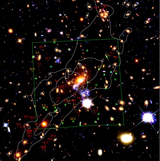
Overview of all multiple-image systems used in this study. The most secure identifications, used to optimize the lens model in the image plane (65 images) are shown in red; in orange we highlight the systems with a spectroscopic redshift from either GMOS or MUSE, with larger green circles highlighting the background sources with a MUSE redshift. System #1 is split into 24 individual sources at the same redshift, not labelled on the figure for clarity (see Table 1 for their coordinates). The underlying colour image is a composite created from HST/ACS images in the F814W, F606W, and F435W passbands. Critical lines at z = 1.49 and 7.0 are shown in white. The green rectangle highlights the VLT/MUSE field of view. The top left-hand inset shows a close-up view of the northern component of the cluster (clump #4 in Table 5). North is up and east is left.
2.2 Spectroscopy with GMOS
MACS J1149 was observed with the GMOS spectrograph on Gemini-North (ID program: GN-2010A-Q-8) during four nights between 2010 March 19 and April 20. The seeing varied between 0.7 and 0.9 arcsec. A single multi-object mask was used with a total of 20 slits covering multiple images, cluster members, and other background galaxies identified from the HST images; the slit width was 1 arcsec. Observations with the B600 and R831 gratings provided a spectral resolution between 1500 at 650 nm and 3000 at 840 nm. A total of 40 × 1050 s exposures were taken, equally split across four wavelength settings centred at 540, 550, 800, and 810 nm.
The GMOS spectroscopic data were reduced using the Gemini iraf reduction package (v. 1.1) to create individual calibrated 2D spectra of each slit and exposure. These were then aligned and combined using standard iraf recipes, and 1D spectra were extracted at the location of the sources of interest.
2.3 Spectroscopy with MUSE
The integral field spectrograph MUSE (Bacon et al. 2010) on the VLT observed the very central region of MACS J1149 (green square in Fig. 1) on 2015 February 14 and March 21 as part of the DDT program 294.A-5032(A) (PI: Grillo). The spectrograph's 1 × 1 arcmin2 field of view was rotated slightly to a position angle of 4|$\deg$|in order to include the majority of the central multiple-image systems. The seeing varied between 0.9 and 1.2 arcsec.
For the analysis presented here, we combine 10 exposures of 1440 s each that are publicly available from the ESO archive (the complete observations were published while this paper was under review; Grillo et al. 2015). We reduced these data using version 1.1 of the MUSE data reduction pipeline (Weilbacher et al., in preparation); selected results from the full data set (including proprietary exposures) are presented by Karman et al. (2015). We performed the basic calibrations (bias and flat-field corrections, wavelength and geometrical calibration) and applied a twilight and illumination correction to the data taken on each night. Flux calibration was performed using a standard star taken at the beginning of the night, and a global sky subtraction was applied to the pixel tables before a final resampling. The 10 exposures were then aligned after adjustments for offsets measured from the centroid of the brightest star in the south of the field (Fig. 2).
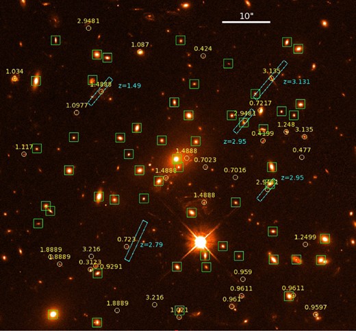
HST/ACS F814W image of MACS J1149 centred on the MUSE field of view. Cyan slits mark GMOS spectroscopic measurements; yellow circles show the sources with MUSE spectroscopic redshifts; and green squares highlight cluster members with a MUSE spectroscopic redshift as listed in Table 1. We note the presence of a small group of galaxies at z = 0.96 in the south-west corner.
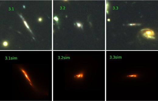
Top panels: HST ACS/WFC3 colour images of system 3 (F814W, F105W, and F160W filters as RGB). Bottom panels: predicted images from a source matching the morphology of image 3.1.
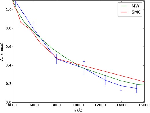
Extinction estimated from a comparison of image 3.3 and image 3.1, and models assuming a MW or SMC extinction law, with attenuations AV = 0.51 and 0.47, respectively.
The final MUSE data cube has a spatial pixel scale of 0.2 arcsec and covers the wavelength range 4750–9350 Å at 1.25 Å pixel−1 and a resolution of 1500–3000. Following Richard et al. (2015), we analysed this large data set using two complementary approaches: we first extracted the 1D spectrum at the location of each of the sources detected in the HFF images and falling within the MUSE field of view, and then estimated all possible redshifts based on emission- and absorption-line features. In addition, we used narrow-band images created with customized software based on SExtractor (Bertin & Arnouts 1996) to perform a blind search of the data cube for isolated emission lines not associated with continuum sources. We then merged the results from both approaches to generate a final MUSE redshift catalogue.
In total, we measured the redshift of 88 sources, including 57 cluster members between z = 0.513 and 0.570, and 27 background sources (some of them being multiply imaged, see Section 3.2). Tables 1– 3 list coordinates and redshifts for cluster members, singly imaged background sources, and foreground galaxies, respectively. The redshifts for multiple images are provided in Table 4.
Catalogue of cluster members detected with VLT/MUSE observations.
| ID | RA | Dec. | zspec |
|---|---|---|---|
| 1 | 177.39548 | 22.404037 | 0.5133 |
| 2 | 177.39328 | 22.400253 | 0.5134 |
| 3 | 177.39859 | 22.398064 | 0.5264 |
| 4 | 177.39096 | 22.401691 | 0.5272 |
| 5 | 177.40628 | 22.405381 | 0.5277 |
| 6 | 177.40358 | 22.396369 | 0.5307 |
| 7 | 177.40745 | 22.399136 | 0.5307 |
| 8 | 177.39121 | 22.392715 | 0.531 |
| 9 | 177.40261 | 22.396186 | 0.5315 |
| 10 | 177.39287 | 22.397096 | 0.5322 |
| 11 | 177.40546 | 22.397881 | 0.5327 |
| 12 | 177.40121 | 22.400339 | 0.5327 |
| 13 | 177.39181 | 22.405281 | 0.5335 |
| 14 | 177.3911 | 22.404904 | 0.5335 |
| 15 | 177.40306 | 22.404389 | 0.5335 |
| 16 | 177.39846 | 22.405383 | 0.536 |
| 17 | 177.39854 | 22.389783 | 0.536 |
| 18 | 177.39965 | 22.399616 | 0.536 |
| 19 | 177.39139 | 22.401063 | 0.5365 |
| 20 | 177.39502 | 22.39602 | 0.5365 |
| 21 | 177.3938 | 22.402294 | 0.5385 |
| 22 | 177.40752 | 22.403047 | 0.5392 |
| 23 | 177.39686 | 22.392292 | 0.5398 |
| 24 | 177.40077 | 22.396256 | 0.5403 |
| 25 | 177.40104 | 22.397885 | 0.5403 |
| 26 | 177.40515 | 22.399789 | 0.5408 |
| 27 | 177.39581 | 22.393496 | 0.5408 |
| 28 | 177.39215 | 22.401282 | 0.5408 |
| 29 | 177.39869 | 22.392303 | 0.5411 |
| 30 | 177.3987 | 22.398519 | 0.5411 |
| 31 | 177.39452 | 22.400647 | 0.5416 |
| 32 | 177.39886 | 22.401818 | 0.5418 |
| 33 | 177.40014 | 22.394428 | 0.5425 |
| 34 | 177.39527 | 22.401054 | 0.5426 |
| 35 | 177.40171 | 22.398803 | 0.5428 |
| 36 | 177.40367 | 22.391933 | 0.5433 |
| 37 | 177.39483 | 22.392927 | 0.5436 |
| 38 | 177.39169 | 22.390611 | 0.5436 |
| 39 | 177.40225 | 22.399759 | 0.5436 |
| 40 | 177.38969 | 22.392704 | 0.5441 |
| 41 | 177.4069 | 22.39583 | 0.5441 |
| 42 | 177.39778 | 22.395445 | 0.5443 |
| 43 | 177.39269 | 22.394364 | 0.5453 |
| 44 | 177.39752 | 22.39955 | 0.5458 |
| 45 | 177.40663 | 22.395536 | 0.5466 |
| 46 | 177.4037 | 22.404578 | 0.5468 |
| 47 | 177.40737 | 22.394819 | 0.547 |
| 48 | 177.39797 | 22.401045 | 0.5471 |
| 49 | 177.40369 | 22.389101 | 0.5491 |
| 50 | 177.40645 | 22.389565 | 0.5496 |
| 51 | 177.39265 | 22.392733 | 0.5504 |
| 52 | 177.39693 | 22.39297 | 0.5511 |
| 53 | 177.39761 | 22.402875 | 0.5511 |
| 54 | 177.39275 | 22.398072 | 0.5519 |
| 55 | 177.38943 | 22.393942 | 0.5554 |
| 56 | 177.39983 | 22.397255 | 0.5609 |
| 57 | 177.40397 | 22.403094 | 0.567 |
Catalogue of singly imaged background galaxies detected with VLT/MUSE observations.
| ID | RA | Dec. | zspec |
|---|---|---|---|
| 58 | 177.39503 | 22.397460 | 0.7016 |
| 59 | 177.39691 | 22.398059 | 0.7023 |
| 60 | 177.39346 | 22.401332 | 0.7217 |
| 61 | 177.40183 | 22.393461 | 0.723 |
| 62 | 177.40377 | 22.392353 | 0.9291 |
| 63 | 177.39456 | 22.391586 | 0.959 |
| 64 | 177.39000 | 22.389538 | 0.9597 |
| 65 | 177.39525 | 22.390021 | 0.961 |
| 66 | 177.39141 | 22.390644 | 0.9611 |
| 67 | 177.39465 | 22.390637 | 0.9611 |
| 68 | 177.39854 | 22.389384 | 1.021 |
| 69 | 177.40885 | 22.403175 | 1.034 |
| 70 | 177.40100 | 22.404706 | 1.087 |
| 71 | 177.40495 | 22.401208 | 1.0977 |
| 72 | 177.40825 | 22.398792 | 1.117 |
| 73 | 177.39185 | 22.400103 | 1.248 |
| 74 | 177.39065 | 22.393606 | 1.2499 |
Catalogue of foreground galaxies detected with VLT/MUSE observations.
| ID | RA | Dec. | zspec |
|---|---|---|---|
| 75 | 177.40410 | 22.392153 | 0.3123 |
| 76 | 177.39331 | 22.399581 | 0.4199 |
| 77 | 177.39704 | 22.404475 | 0.424 |
| 78 | 177.39088 | 22.398611 | 0.477 |
| ID | RA | Dec. | zspec |
|---|---|---|---|
| 75 | 177.40410 | 22.392153 | 0.3123 |
| 76 | 177.39331 | 22.399581 | 0.4199 |
| 77 | 177.39704 | 22.404475 | 0.424 |
| 78 | 177.39088 | 22.398611 | 0.477 |
Multiply imaged systems considered in this work.
| ID | RA | Dec. | z | mF814W | μ |
|---|---|---|---|---|---|
| 1.1a | 177.397 | 22.396007 | 1.4888 | 22.46 ± 0.01 | 3.7 ± 0.1 |
| 1.2a | 177.39941 | 22.397438 | 1.4888 | 23.39 ± 0.01 | 4.1 ± 0.1 |
| 1.3a | 177.40341 | 22.402426 | 1.4888 | 22.73 ± 0.01 | 9.7 ± 0.3 |
| 2.1 | 177.40243 | 22.389739 | 1.894 | 26.46 ± 0.02 | 4.6 ± 0.1 |
| 2.2 | 177.40607 | 22.392484 | 1.894 | 24.4 ± 0.01 | >20 |
| 2.3 | 177.40657 | 22.392881 | 1.894 | 24.49 ± 0.01 | 18.5 ± 1.6 |
| 3.1 | 177.39076 | 22.39984 | 3.128 | 23.36 ± 0.0 | 10.5 ± 0.4 |
| 3.2 | 177.39272 | 22.403074 | 3.128 | 22.77 ± 0.0 | 10.3 ± 0.4 |
| 3.3 | 177.40129 | 22.407182 | 3.128 | 24.01 ± 0.01 | 4.3 ± 0.1 |
| 4.1 | 177.39301 | 22.396826 | 2.95 | 25.41 ± 0.01 | – |
| 4.2 | 177.3944 | 22.400729 | 2.95 | – | 7.4 ± 0.2 |
| 4.3 | 177.40419 | 22.40612 | 2.95 | 25.96 ± 0.03 | 3.4 ± 0.1 |
| 5.1 | 177.39976 | 22.393062 | 2.79 | 25.15 ± 0.01 | 15.5 ± 0.7 |
| 5.2 | 177.40111 | 22.393824 | 2.79 | 25.01 ± 0.01 | 12.0 ± 0.5 |
| 5.3 | 177.40794 | 22.403538 | 2.79 | 26.12 ± 0.02 | 4.3 ± 0.1 |
| 6.1 | 177.39972 | 22.392545 | 2.66 ± 0.02 | 26.37 ± 0.03 | 9.0 ± 0.3 |
| 6.2 | 177.40181 | 22.393858 | – | 26.4 ± 0.02 | 8.1 ± 0.3 |
| 6.3 | 177.40804 | 22.402505 | – | 27.41 ± 0.06 | 4.7 ± 0.1 |
| 7.1 | 177.39895 | 22.391332 | 2.79 ± 0.02 | 25.87 ± 0.02 | 4.5 ± 0.1 |
| 7.2 | 177.40339 | 22.394269 | – | 26.16 ± 0.02 | 4.6 ± 0.1 |
| 7.3 | 177.40759 | 22.401243 | – | 26.3 ± 0.03 | 4.2 ± 0.1 |
| 8.1 | 177.39849 | 22.394351 | 2.81 ±0.02 | 26.12 ± 0.02 | >20 |
| 8.2 | 177.39978 | 22.395055 | – | 24.7 ± 0.04 | 15.1 ± 0.6 |
| 8.3 | 177.40709 | 22.40472 | – | 26.03 ± 0.02 | 3.2 ± 0.1 |
| 9.1 | 177.40515 | 22.426221 | 0.981 | 24.81 ± 0.01 | 1.7 ± 0.1 |
| 9.2 | 177.40387 | 22.427217 | 0.981 | 24.57 ± 0.01 | 4.9 ± 1.3 |
| 9.3 | 177.40323 | 22.427221 | 0.981 | 24.14 ± 0.0 | 2.9 ± 0.3 |
| 9.4 | 177.40365 | 22.426408 | 0.981 | 25.11 ± 0.01 | 3.4 ± 0.3 |
| 10.1 | 177.40447 | 22.425508 | 1.34 ± 0.01 | 25.99 ± 0.01 | 3.0 ± 0.2 |
| 10.2 | 177.40362 | 22.425629 | – | 26.09 ± 0.01 | 2.2 ± 0.1 |
| 10.3 | 177.4022 | 22.426611 | – | 26.5 ± 0.02 | 1.8 ± 0.1 |
| 13.1 | 177.4037 | 22.397787 | 1.28 ± 0.01 | 25.87 ± 0.03 | >20 |
| 13.2 | 177.40282 | 22.396656 | – | 26.14 ± 0.02 | 11.9 ± 0.6 |
| 13.3 | 177.40003 | 22.393857 | – | 25.78 ± 0.02 | 5.3 ± 0.1 |
| 14.1 | 177.39166 | 22.403504 | 3.50 ± 0.06 | 27.06 ± 0.03 | 13.4 ± 0.7 |
| 14.2 | 177.39084 | 22.402624 | – | 27.13 ± 0.03 | >20 |
| 15.1 | 177.40922 | 22.387695 | 3.58 ± 0.08 | 26.57 ± 0.03 | 7.5 ± 0.9 |
| 15.2 | 177.41034 | 22.388745 | – | 25.86 ± 0.02 | >20 |
| 15.3 | 177.40624 | 22.385349 | – | 27.19 ± 0.04 | 3.8 ± 0.1 |
| 16.1 | 177.40971 | 22.387662 | 2.65 ± 1.45 | 27.19 ± 0.04 | >20 |
| 16.2 | 177.40989 | 22.387828 | – | 27.34 ± 0.04 | >20 |
| 17.1 | 177.40994 | 22.387232 | 6.28 ± 0.17 | 28.02 ± 0.06 | 5.5 ± 0.4 |
| 17.2 | 177.41124 | 22.388457 | – | 28.14 ± 0.07 | 15.2 ± 1.1 |
| 17.3 | 177.40658 | 22.384483 | – | 28.46 ± 0.08 | 3.6 ± 0.1 |
| 18.1 | 177.40959 | 22.38666 | 7.76 ± 0.16 | 28.51 ± 0.23 | 3.4 ± 0.2 |
| 18.2 | 177.41208 | 22.389057 | – | – | 8.3 ± 0.3 |
| 18.3 | 177.40669 | 22.384319 | – | – | 3.6 ± 0.1 |
| 21.1 | 177.39284 | 22.41287 | 2.48 ± 0.04 | 26.38 ± 0.02 | >20 |
| 21.2 | 177.39353 | 22.413083 | – | 22.52 ± 0.06 | >20 |
| 21.3 | 177.39504 | 22.412686 | – | 27.5 ± 0.04 | 14.6 ± 1.1 |
| 22.1 | 177.40402 | 22.3929 | 3.216 | 27.86 ± 0.05 | 5.0 ± 0.2 |
| 22.2 | 177.40906 | 22.400233 | 3.216 | 27.85 ± 0.05 | 3.9 ± 0.1 |
| 22.3 | 177.40016 | 22.39015 | 3.216 | 27.57 ± 0.05 | 4.1 ± 0.1 |
| 26.1 | 177.40475 | 22.425978 | 1.49 ± 0.03 | 26.87 ± 0.03 | 3.5 ± 0.4 |
| 26.2 | 177.40361 | 22.426078 | – | 26.44 ± 0.03 | 4.0 ± 0.5 |
| 26.3 | 177.40274 | 22.426936 | – | 26.7 ± 0.02 | 2.5 ± 0.1 |
| 29.1 | 177.40799 | 22.389056 | 2.76 ± 0.05 | 27.99 ± 0.07 | 10.7 ± 2.0 |
| 29.2 | 177.40907 | 22.390406 | – | 27.55 ± 0.04 | 9.2 ± 0.4 |
| 29.3 | 177.40451 | 22.386702 | – | 28.56 ± 0.08 | 4.0 ± 0.1 |
| 31.1 | 177.40215 | 22.396747 | 2.78 ± 0.03 | 26.86 ± 0.03 | 2.3 ± 0.1 |
| 31.2 | 177.39529 | 22.391833 | – | 26.2 ± 0.02 | 3.2 ± 0.1 |
| 31.3 | 177.40562 | 22.402439 | – | 26.1 ± 0.02 | 4.2 ± 0.1 |
| 34.1 | 177.4082 | 22.388116 | 3.42 ± 0.08 | 27.28 ± 0.04 | 4.3 ± 0.5 |
| 34.2 | 177.41037 | 22.390621 | – | 27.35 ± 0.05 | 6.7 ± 0.2 |
| 34.3 | 177.40518 | 22.386031 | – | 27.66 ± 0.06 | 4.0 ± 0.1 |
| 1002.2b | 177.39701 | 22.396 | 1.4888 | – | – |
| 1002.3b | 177.39943 | 22.397424 | 1.4888 | – | – |
| 1002.1b | 177.40343 | 22.402419 | 1.4888 | – | – |
| 1003.2b | 177.39815 | 22.396344 | 1.4888 | – | – |
| 1003.3b | 177.39927 | 22.39683 | 1.4888 | – | – |
| 1003.1b | 177.40384 | 22.402564 | 1.4888 | – | – |
| 1004.2b | 177.39745 | 22.396397 | 1.4888 | – | – |
| 1004.3b | 177.39916 | 22.397214 | 1.4888 | – | – |
| 1004.1b | 177.40359 | 22.402653 | 1.4888 | – | – |
| 1006.2b | 177.39712 | 22.396717 | 1.4888 | – | – |
| 1006.3b | 177.39812 | 22.398247 | 1.4888 | – | – |
| 1006.4b | 177.39878 | 22.397625 | 1.4888 | – | – |
| 1006.1b | 177.40338 | 22.402867 | 1.4888 | – | – |
| 1007.2b | 177.39697 | 22.396636 | 1.4888 | – | – |
| 1007.3b | 177.39782 | 22.398464 | 1.4888 | – | – |
| 1007.4b | 177.39882 | 22.397711 | 1.4888 | – | – |
| 1007.1b | 177.40329 | 22.402831 | 1.4888 | – | – |
| 1008.2b | 177.39698 | 22.396553 | 1.4888 | – | – |
| 1008.3b | 177.39793 | 22.398418 | 1.4888 | – | – |
| 1008.4b | 177.39889 | 22.397639 | 1.4888 | – | – |
| 1008.1b | 177.40331 | 22.402786 | 1.4888 | – | – |
| 1009.2b | 177.397 | 22.396444 | 1.4888 | – | – |
| 1009.1b | 177.399 | 22.397625 | 1.4888 | – | – |
| 1010.2b | 177.39694 | 22.396394 | 1.4888 | – | – |
| 1010.1b | 177.39904 | 22.397611 | 1.4888 | – | – |
| 1011.2b | 177.39701 | 22.396197 | 1.4888 | – | – |
| 1011.3b | 177.39922 | 22.397472 | 1.4888 | – | – |
| 1011.1b | 177.40337 | 22.402556 | 1.4888 | – | – |
| 1015.2b | 177.39672 | 22.395372 | 1.4888 | – | – |
| 1015.3b | 177.39975 | 22.397489 | 1.4888 | – | – |
| 1015.4b | 177.40012 | 22.397203 | 1.4888 | – | – |
| 1015.1b | 177.40325 | 22.402008 | 1.4888 | – | – |
| 1016.2b | 177.39688 | 22.396211 | 1.4888 | – | – |
| 1016.3b | 177.39918 | 22.397589 | 1.4888 | – | – |
| 1016.1b | 177.40327 | 22.402581 | 1.4888 | – | – |
| 1018.2b | 177.39723 | 22.396208 | 1.4888 | – | – |
| 1018.3b | 177.39933 | 22.397303 | 1.4888 | – | – |
| 1018.1b | 177.40354 | 22.402533 | 1.4888 | – | – |
| 1019.2b | 177.39661 | 22.396308 | 1.4888 | – | – |
| 1019.3b | 177.39777 | 22.398783 | 1.4888 | – | – |
| 1019.4b | 177.39867 | 22.398219 | 1.4888 | – | – |
| 1019.5b | 177.39899 | 22.397869 | 1.4888 | – | – |
| 1019.1b | 177.40303 | 22.402681 | 1.4888 | – | – |
| 1020.2b | 177.39708 | 22.395722 | 1.4888 | – | – |
| 1020.1b | 177.40353 | 22.402236 | 1.4888 | – | – |
| 1021.2b | 177.39689 | 22.395761 | 1.4888 | – | – |
| 1021.3b | 177.39954 | 22.397483 | 1.4888 | – | – |
| 1021.4b | 177.39996 | 22.397094 | 1.4888 | – | – |
| 1021.1b | 177.40336 | 22.402289 | 1.4888 | – | – |
| 1022.2b | 177.39717 | 22.396508 | 1.4888 | – | – |
| 1022.3b | 177.39895 | 22.397503 | 1.4888 | – | – |
| 1022.1b | 177.40342 | 22.402764 | 1.4888 | – | – |
| 1024.2b | 177.39809 | 22.395853 | 1.4888 | – | – |
| 1024.3b | 177.39993 | 22.396714 | 1.4888 | – | – |
| 1024.1b | 177.40379 | 22.402193 | 1.4888 | – | – |
| 1026.2b | 177.39798 | 22.396011 | 1.4888 | – | – |
| 1026.3b | 177.39981 | 22.39676 | 1.4888 | – | – |
| 1026.1b | 177.40379 | 22.402317 | 1.4888 | – | – |
| 1050.2b | 177.39746 | 22.395653 | 1.4888 | – | – |
| 1050.3b | 177.39761 | 22.395778 | 1.4888 | – | – |
| 1050.4b | 177.39775 | 22.395217 | 1.4888 | – | – |
| 1050.5b | 177.39818 | 22.395681 | 1.4888 | – | – |
| 1050.6b | 177.40006 | 22.396691 | 1.4888 | – | – |
| 1050.1b | 177.40376 | 22.402033 | 1.4888 | – | – |
| 1052.2b | 177.3973 | 22.395383 | 1.4888 | – | – |
| 1052.3b | 177.39792 | 22.395725 | 1.4888 | – | – |
| 1052.4b | 177.39803 | 22.395239 | 1.4888 | – | – |
| 1052.5b | 177.39817 | 22.395478 | 1.4888 | – | – |
| 1052.6b | 177.40016 | 22.396758 | 1.4888 | – | – |
| 1052.1b | 177.4037 | 22.401947 | 1.4888 | – | – |
| 1192.2b | 177.39664 | 22.396236 | 1.4888 | – | – |
| 1192.3b | 177.39796 | 22.398689 | 1.4888 | – | – |
| 1192.4b | 177.39904 | 22.397833 | 1.4888 | – | – |
| 1192.1b | 177.40305 | 22.402631 | 1.4888 | – | – |
| 1211.2b | 177.39699 | 22.395628 | 1.4888 | – | – |
| 1211.1b | 177.40346 | 22.402172 | 1.4888 | – | – |
| 1222.2b | 177.39698 | 22.396081 | 1.4888 | – | – |
| 1222.1b | 177.4034 | 22.402461 | 1.4888 | – | – |
Notes. We include the predicted magnification given by our model. Some of the magnitudes are not quoted because we were facing deblending issues that did not allow us to get reliable measurements. The flux magnification factors come from our best-fitting mass model, with errors derived from MCMC sampling.
aThanks to the VLT/MUSE data, we were able to revise spectroscopic redshift of system #1, from z = 1.491, as in Smith et al. (2009), to z = 1.4888.
bIndicate the different components of system #1 we have used for our model, following the decomposition presented in Rau et al. (2014).
3 MULTIPLY IMAGED SYSTEMS
3.1 HST identifications
MACS J1149 has been the subject of a number of strong-lensing analyses (Smith et al. 2009; Zitrin & Broadhurst 2009; Zitrin et al. 2011; Johnson et al. 2014; Rau et al. 2014; Richard et al. 2014; Coe et al. 2015; Diego et al. 2016; Oguri 2015; Sharon & Johnson 2015), all of which were based on pre-HFF data except for Diego et al. (2016), their work uses one-third of the HFF data. We started our search for multiple images guided by the mass model of Richard et al. (2014). This model incorporates 35 multiple images of 10 different lensed galaxies, three of which have spectroscopic redshifts from Smith et al. (2009): systems #1, #2, and #3, at z = 1.491, 1.894, and 2.497, respectively.
The new, deep HFF ACS and WFC3 images allow us to extend this set of multiple images. To this end, we followed Jauzac et al. (2014, 2015) and first computed the cluster's gravitational-lensing deflection field that describes the mapping of images from the image plane to the source plane, on a grid with a spacing of 0.2 arcsec pixel−1. Since the transformation scales with redshift as described by the distance ratio DLS/DOS, where DLS and DOS are the distances between the lens and the source, and the observer and the source, respectively, it is only computed once, thereby enabling an efficient lens inversion. We then compute the critical region at redshift z = 7 and limit our search for multiple images in the ACS data to this area (white contours in Fig. 1). Careful searches, combined with visual scrutiny and confirmation, revealed 12 new multiply imaged systems, bringing the total number of multiple images identified in MACS J1149 to 65, involving 22 different multiply imaged galaxies (Fig. 1 and Table 4), which leads to considerable tighter constraints on the mass model of the cluster. Although a significant improvement over the pre-HFF statistics, this number of new systems is disappointing compared to how many were discovered in the first two HFF clusters, MACS J0416.1−2403 and Abell 2744; we discuss this issue in Section 5.1.
As one of the main goals of our analysis is to measure precise time delays prompted by the discovery of SN Refsdal, we followed Rau et al. (2014) and decomposed system #1, the SN host galaxy, into 24 features, selected as the brightest components of the spiral (see the bottom part of Table 4 for their coordinates). We also added the four images of SN Refsdal located in image 1.2 and labelled S1, S2, S3, and S4, following the same notation as Kelly et al. (2015a), Sharon & Johnson (2015), and Oguri (2015).
Flux measurements were derived from isophotal magnitudes measured with SExtractor (Bertin & Arnouts 1996), and the fluxes of oversegmented multiple images were combined into a total flux per multiple image. The corresponding magnitudes are presented in Table 4. Combining all HFF filters, we find acceptable values for χ2 (∼1–3) for almost all images, with slightly high values typically being observed for sources whose photometry is compromised by bright nearby sources.
A notable exception is image 3.3, already found in the pre-HFF images, which features a very high χ2 value (56), although it seems to be the most plausible counterimage of system 3 based on predictions of both its position and morphology derived from a lensing model constrained with 3.1 and 3.2 only. Fig. 3 shows the three images of system #3 in composite HST ACS/WFC3 colour images (top panel), as well as the predicted images (monochrome), simulated based on the morphology of image 3.1. The predicted location and morphology of images 3.2 and 3.3 closely match those of the real data; however, the colour of image 3.3 is significantly reddened compared to images 3.1 and 3.2, thus producing the aforementioned large χ2 value. Removing the differential amplification between images 3.1 and 3.3, we find the magnitude differences in all filters to follow a typical reddening curve (Fig. 4), which can be easily modelled by a Milky Way (MW; Allen 1976) or Small Magellanic Cloud (SMC; Prevot et al. 1984; Bouchet et al. 1985) extinction curve, with typical values of AV = 0.51 (MW) or 0.47 (SMC), if we assume that the extinction occurs in the cluster at z = 0.54. Dust extinction has been previously reported in the outskirts of clusters (e.g. Chelouche, Koester & Bowen 2007). Alternatively, we cannot rule out dust extinction by an intervening galaxy in the foreground or background of the cluster. For instance, the background spiral to the lower right of image 3.3 (Fig. 3) is a good candidate. We derive a photometric redshift z = 1.4 and a best-fitting extinction AV = 1.0 from the public CLASH photometric catalogues (Postman et al. 2012)4 using the hyperz photometric redshift software (Bolzonella, Miralles & Pelló 2000). Image 3.3 is located 12 kpc from the centre of this galaxy in the source plane at z = 1.4; at such a high impact parameter the lower extinction in image 3.3 can thus be expected.
3.2 Redshift constraints
The spectroscopic observations described in Section 2 allowed us to confirm newly identified multiple-image systems, as well as to correct earlier spectroscopic redshifts measurements. Compared to Smith et al. (2009), we revise the spectroscopic redshift of system #3 to z = 3.128, based on the deeper GMOS data that clearly show Lyman α in emission as well as an associated spectral Lyman α break in the continuum (Fig. 5). The revised redshift of system #3 is also confirmed with MUSE for images 3.1 and 3.2. We also measure secure GMOS spectroscopic redshifts for system #4, z = 2.95, for system #5, z = 2.79, and system #9, z = 0.981, from strong Lyman α and [O ii] emission lines, respectively. MUSE observations add to these findings by revealing extended emission around image 4.1, producing a Lyman α Einstein ring around the very close cluster member (Fig. 6). MUSE observations also confirm the redshift of the HFF multiple-image system #22 as z = 3.216, again from strong Lyman α emission. Finally, we slightly revise the redshift of the system #1, the face-on spiral, to z = 1.4888, based on the total integral field unit (IFU) spectrum of this object (see also Yuan et al. 2011).
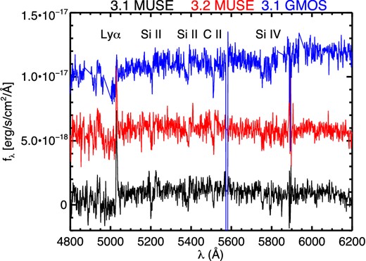
Example of extracted GMOS and MUSE spectra for system 3, confirming a redshift z = 3.128 from Lyman α in emission, spectral break, and UV absorption lines. Individual spectra are offset vertically for clarity.

Close-up view of system #4. The left-hand panel highlights images 4.1 and 4.2 in the HST/ACS image. The right-hand panel shows the Lyman α emission in the same area as observed with MUSE.
In addition to measuring the redshifts of known multiple-image systems, we used the spectroscopic redshifts measured from GMOS and MUSE data also to investigate the possible multiplicity of other background sources (see second part of Table 2). All of these are predicted by our best mass model (Section 4) to be single images, including a small group of 11 galaxies at 0.95 < z < 1.3 within the MUSE field of view (Fig. 2 and Table 2). This test allowed us to reject potential new multiple images and to confirm the validity of our strong-lensing analysis.
Table 4 lists the coordinates, redshifts (spectroscopic or predicted by our model), F814W-band magnitudes, and magnifications predicted by our best-fitting model, for all multiple images used in this work. Magnitudes were measured using SExtractor (Bertin & Arnouts 1996).
4 STRONG-LENSING MASS MODEL
4.1 Methodology
Since our method to create the MACS J1149 mass model closely follows the one used by Jauzac et al. (2014, 2015), we here only give a brief summary and refer the reader to Kneib et al. (1996), Smith et al. (2005), Verdugo et al. (2011), and Richard et al. (2011b) for more details. Our mass model combines large-scale dark matter haloes to model the cluster-scale mass components and galaxy-scale haloes to model individual cluster members, typically large elliptical galaxies or galaxies that affect strong-lensing features due to their proximity to multiple images. As in our previous work, all mass components are modelled as Pseudo Isothermal Elliptical Mass Distribution (PIEMD; Limousin, Kneib & Natarajan 2005; Jauzac et al. 2014, 2015), characterized by a velocity dispersion σ, a core radius rcore, and a cut radius rcut. In this parametric approach, haloes are not allowed to contain zero mass, and hence the relative probability of different models meeting the observational constraints is quantified by the χ2 and rms statistics.
For the PIEMD models added to parametrize cluster members (mass perturbers) we fix the PIEMD parameters (centre, ellipticity, and position angle) at the values measured from the cluster light distribution (see e.g. Kneib et al. 1996; Limousin et al. 2007; Richard et al. 2011a) and assume empirical scaling relations to relate the dynamical PIEMD parameters (velocity dispersion and cut radius) to the galaxies’ observed luminosity (Richard et al. 2014). For an L* galaxy, we optimize the velocity dispersion between 100 and 250 km s−1 and force the cut radius to less than 70 kpc to account for tidal stripping of galactic dark matter haloes (Limousin et al. 2007, 2009; Natarajan et al. 2009; Wetzel & White 2010).
Finally, one more parameter that is fixed, but plays an important role in the χ2 computation, is the positional uncertainty of the multiple images. Indeed, it will affect the derivation of errors, i.e. a smaller positional uncertainty will generally result in a smaller statistical uncertainty, thus leading to an underestimation of the statistical error budget.
With HFF-like data, the average astrometric precision of the image position is of the order of 0.05 arcsec. However, parametric cluster lens models often fail to reproduce or predict image positions to this precision, yielding instead typical image plane rms values between 0.2 arcsec and a few arcseconds. In this work, we use a positional uncertainty of 0.5 arcsec.
4.2 Results
Our mass model includes five cluster-scale haloes, referred to as #1, #2, #3, #4, and #5 in Table 5. An additional cluster-scale halo, south-east of the BCG, was requested by the model compare to the pre-HFF mass model presented in Richard et al. (2014). Indeed, its necessity was confirmed by both a smaller rms value and a better reduced χ2 compare to a four cluster-scale haloes mass model. During the optimization process, the position of these large-scale haloes is allowed to vary within 20 arcsec of the associated light peak. In addition, we limit the ellipticity, defined as e = (a2 + b2)/(a2 − b2), to values below 0.7, while the core radius and the velocity dispersion are allowed to vary between 1 and 35 arcsec, and 100 and 2000 km s−1, respectively. The cut radius, by contrast, is fixed at 1000 kpc, since strong-lensing data alone do not probe the mass distribution on such large scales. In addition to these five cluster-scale dark matter haloes, we include galaxy-scale perturbations induced by 216 probable cluster members (Richard et al. 2014) by assigning a galaxy-scale halo to each of them. Finally, we add two galaxy-scale haloes to model the BCG of the cluster (clump #6 in Table 5), as well as the cluster member lensing SN Refsdal (clump #7 in Table 5). Using the set of the most securely identified multiply imaged galaxies described in Section 3 and shown in Fig. 1, we optimize the free parameters of this mass model using the publicly available lenstool software.5
PIEMD parameters inferred for the five dark matter clumps considered in the optimization procedure. Clumps #6 and #7 are galaxy-scale haloes that were modelled separately from scaling relations, to respectively model the BCG of the cluster as well as the cluster member responsible for the four multiple images of SN Refsdal. Coordinates are given in arcseconds with respect to α = 177.3987300, δ = 22.3985290. The ellipticity e is the one of the mass distribution, in units of (a2 + b2)/(a2 − b2). The position angle θ is given in degrees and is defined as the direction of the semimajor axis of the iso-potential, counted counterclockwise from the horizontal axis (being the RA axis). Error bars correspond to the 1σ confidence level. Parameters in brackets are not optimized. Concerning the scaling relations, the reference magnitude is magF814W = 20.65.
| Clump | Δx | Δy | e | θ | rcore (kpc) | rcut (kpc) | σ (km s−1) |
|---|---|---|---|---|---|---|---|
| #1 | |$-1.95^{+ 0.10}_{-0.19}$| | 0.17 |$^{+ 0.15}_{-0.22}$| | 0.58 ± 0.01 | 30.58|$^{+ 0.35}_{-0.51}$| | 112.9|$^{+ 3.6}_{-2.1}$| | [1000] | 1015|$^{+ 7}_{-6}$| |
| #2 | −28.02|$^{+ 0.26}_{-0.17}$| | −36.02|$^{+ 0.27}_{-0.21}$| | 0.70 ± 0.02 | 39.02|$^{+ 2.23}_{-1.69}$| | 16.5|$^{+ 2.7}_{-3.9}$| | [1000] | 331|$^{+ 13}_{-9}$| |
| #3 | |$-48.65^{+ 0.13}_{-0.49}$| | |$-51.35^{+ 0.30}_{-0.22}$| | 0.35 ± 0.02 | 126.48|$^{+ 7.11}_{-4.42}$| | 64.2|$^{+ 6.8}_{-9.6}$| | [1000] | 286|$^{+ 24}_{-16}$| |
| #4 | |$17.62^{+ 0.28}_{-0.18}$| | 46.90 |$^{+ 0.36}_{-0.28}$| | 0.15 ± 0.02 | 54.66|$^{+ 3.51}_{-4.83}$| | 110.5|$^{+ 1.2}_{-2.1}$| | [1000] | 688|$^{+ 9}_{-17}$| |
| #5 | |$-17.22^{+ 0.17}_{-0.18}$| | 101.85 |$^{+ 0.08}_{-0.07}$| | 0.44 ± 0.05 | 62.29|$^{+ 5.14}_{-4.61}$| | 2.1|$^{+ 0.5}_{-0.1}$| | [1000] | 263|$^{+ 8}_{-7}$| |
| #6 | [0.0] | [0.0] | [0.2] | [34.0] | 3.95|$^{+ 0.57}_{-0.89}$| | 92.08|$^{+ 6.50}_{-7.91}$| | 284 ± 8 |
| #7 | [3.16] | [−11.10] | 0.22 ± 0.02 | 103.56|$^{+ 7.09}_{-7.95}$| | [0.15] | 43.17|$^{+ 1.34}_{-1.02}$| | 152|$^{+ 2}_{-1}$| |
| L* elliptical galaxy | – | – | – | – | [0.15] | 52.48|$^{+ 2.17}_{-0.89}$| | 148|$^{+ 2}_{-3}$| |
The best-fitting model optimized in the image plane predicts image positions that agree with the observed positions to within an rms of 0.91 arcsec, a value that is slightly higher than the one published in Richard et al. (2014). This increase is in part caused by the high individual χ2 value of image 3.3 (χ2 = 13), which we nonetheless consider a robust identification (see discussion in Section 3).
The parameters describing our best-fitting mass model are listed in Table 5. Although allowed to vary within 20 arcsec of their associated light peak, the final positions of the five cluster-scale haloes predicted by the model coincide much more closely with the light peaks. In order to integrate the mass map within annuli, we choose the location of the overall BCG, i.e. α = 177.3987300, δ = 22.3985290, as the cluster centre. The two-dimensional (cylindrical) mass within 80 arcsec is then M(R < 500 kpc) = (6.29 ± 0.03) × 1014 M⊙, slightly lower than the previous result by Smith et al. (2009) of M(R < 500 kpc) = (6.7 ± 0.4) × 1014 M⊙, but within their error bars. The mass of (1.71 ± 0.20) × 1014 M⊙ within a 30 arcsec (∼200 kpc) aperture reported by Zitrin et al. (2011) agrees with the value from our new mass model of M(R < 200 kpc) = (1.840 ± 0.006) × 1014 M⊙.
5 DISCUSSION
5.1 The lensing power of MACS J1149
The small number of 22 multiple-imaged systems identified in MACS J1149 from HFF data is surprising, compared to the 34 and 51 systems found in equally deep HST images of the first two HFF clusters, Abell 2744 and MACS J0416. Because of this discrepancy, we carefully examined the MUSE data for several sources at z ∼ 1 within the central arcmin2 of the cluster core, but confirmed all of them to be single images, as predicted.
In an attempt to find the root cause of the relatively modest lensing power of MACS J1149, we compute the surface area in the image plane within which we expect multiple images (Fig. 7). For all six Frontier Field clusters we find this area to increase with source redshift, starting at an average value of ∼1 arcmin2 at z = 1 and reaching values around 2.5 arcmin2 at z = 7, although with large cluster-to-cluster differences.
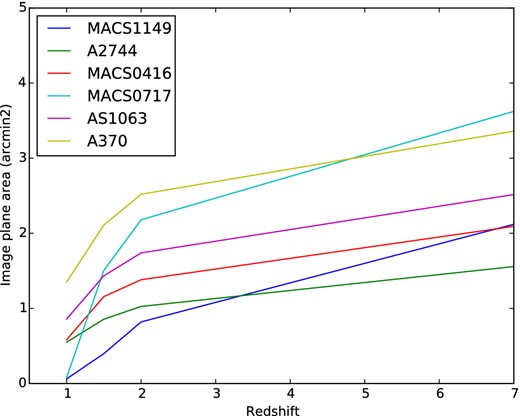
Evolution of the surface area in the image plane within which multiple images are observed, as a function of the source redshift. Compared to the five other Frontier Fields clusters, MACS J1149 features a much smaller multiple-image region at low redshifts.
Whereas the overall shape of these curves is very similar for four of the six HFF clusters, to the extent that they are essentially scaled versions of each other, two systems exhibit a different trend with redshift. For both MACS J1149 and MACS J0717, the curves in Fig. 7 start at a very small surface area at z = 1 (∼0.1 arcmin2) but then rise much more steeply than those of the remaining HFF targets. Part of this effect is due to their being at higher redshift (z = 0.55), causing their corresponding critical surface mass density to decrease more rapidly with increasing source redshift. We argue that the trend is also rooted in both of these clusters sharing a similar morphology or, more generally, in the fact that extremely disturbed clusters (both MACS J0717 and MACS J1149 consist of more than three subclusters) are at a disadvantage for lensing background sources at low redshift, owing to disjoint critical lines, but gain on less complex systems at higher source redshifts at which the critical lines for strong lensing join. Being the much more massive system, MACS J0717 features a larger image plane area throughout though, thereby ‘catching up’ much faster than the less massive MACS J1149.
In conclusion, we trace the small number of multiple images in MACS J1149 to the system's complex and extended morphology which leads to the smallest area for multiple imaging of sources at redshifts z < 3 among all HFF target clusters. Following the same argument, we expect the two final HFF targets, Abell 370 and AS 1063, to produce much larger number of multiple images when they are observed with HST in the coming months.
5.2 SN Refsdal
5.2.1 Different studies of SN Refsdal
Since the discovery of SN Refsdal, three new pre-HFF strong-lensing analyses have attempted to precisely compute the time delays between the multiple images of the SN (Diego et al. 2016; Oguri 2015; Sharon & Johnson 2015), using both parametric and free-form approaches. While this paper was under review, three additional strong-lensing groups have presented predictions using HFF, VLT, and Keck data (Grillo et al. 2015; Kawamata et al. 2015; Treu et al. 2015).6 All the models predict six multiple images of SN Refsdal in total: one in each of the three multiple images of the face-on spiral (1.1, 1.2. 1.3), with the one in image 1.1 quadruply imaged by a cluster member, resulting in four separate components named S1, S2, S3, and S4, as shown in Fig. 8.

Zoom on system #1, with orange circles highlighting the 24 components of the spiral used for our mass model. Left-hand panel: image 1.1 with the Einstein cross formed by images S1, S2, S3, and S4 of SN Refsdal. Middle panel: image 1.2 with the predicted location of SN Refsdal in red, SX, predicted to appear ∼1.8 yr after S1, i.e. in 2016 January. Right-hand panel: image 1.3 with the predicted position of SN Refsdal, SY, where it would have been visible ∼11.5 yr ago following the predictions from our model.
Sharon & Jonhson (2015), Diego et al. (2016) and Oguri (2015). Using lenstool, Sharon & Johnson (2015) investigated different models and found the order of appearance for the four images within image 1.1 to be S3–S1–S2–S4. As for the remaining two images of SN Refsdal, Sharon & Johnson (2015) claim that the first one, SY, appeared in image 1.3 ∼12 yr ago, while the sixth image, SX, is predicted to appear in image 1.2 in 2015 September. By contrast, Oguri (2015), using the public code glafic (Oguri 2010), arrives at a different order of appearance of the SN within image 1.1, namely S1–S3–S2–S4 (see Table 6), claims that SY appeared ∼17 yr ago, and predicts that SX is to appear in 2015 November. Finally, Diego et al. (2016), using a free-form mass modelling technique, WSLAP+ (Diego et al. 2005, 2007; Sendra et al. 2014), do not address the order of appearance of images S1, S2, S3, and S4, but conclude that SY appeared ∼9 yr ago and predict SX to appear between 2015 November and 2016 January.
Treu et al. (2015), Kawamata et al. (2015) and Grillo et al. (2015). More recently, Treu et al. (2015) presented predictions based on seven different mass models. These new measurements were made using HFF mass models, and taking advantage of new spectroscopy coming from HST with GLASS data (PI: Treu), as well as the complete MUSE DDT program 294.A-5032(A) (PI: Grillo; for our model we only had access to 4 h of the data as detailed in Section 2). The teams involved in this analysis (Sharon, Zitrin, Diego, Grillo, and Oguri) identified independently new multiple image systems and then voted to select the most secured identifications following the same criteria as presented in Wang et al. (2015). While our two analyses were done separately, we find a good agreement in terms of new multiple-image systems: system #22, system #29, system #21, system #15, system #16, system #31, system #17, system #18, and system #34 correspond, respectively, to system #110, system #21, system #24, system #26, system #27, system #28, system #203, system #204, and system #205 in Treu et al. (2015). There is no clear discrepancy between our spectroscopic measurements and the ones presented in Treu et al. (2015) and Grillo et al. (2015). However, looking at the cluster members, Treu et al. (2015) present 170 spectroscopic identifications while we only identify 57 (see Sec-tion 2). Grillo et al. (2015) independently presented their strong-lensing mass model, as well as the complete data set they obtained with the MUSE program 294.A-5032(A). Kawamata et al. (2015) also presented the Oguri's models in their paper. The results did not change from the ones presented in Treu et al. (2015).
The five teams involved in the Treu et al. (2015) SN Refsdal analysis predicted time delays for images S1, S2, S3, and S4, with different order of appearance and occurring within 12 and up to 240 d, depending on the model. The appearance of SX at peak brightness is predicted during the first half of 2016, while SY would have appeared between 1994 and 2004. However, magnification estimates from the different models suggest that it would have been too faint to be observable from archival data.
We refer the reader to Table 6 for the exact values of the time delays predicted by these eight different measurements, as well as the ones found by our analysis. For consistency, we use in all cases S1 as our reference and adopt the established naming convention (SX and SY) for the two other images of SN Refsdal in image 1.2 and 1.3, respectively. We note that some of the teams in Treu et al. (2015) had two sets of predictions, as they run different mass models using two different sets of multiple images (‘gold’, the most secured ones, and ‘all’, for the gold images plus a subset of less secured identifications). In Table 6 we keep the same notation as in Treu et al. (2015) to limit confusion.
Time delays obtained for each image of SN Refsdal, given in days. The first part of the table gives the coordinates of the SN images used in this analysis, with the ones for SX and SY predicted by our best-fitting mass model. We also quote the magnification predicted by our best-fitting mass model, μ. The second part of the table presents the time delays we measured with our analysis, following the two different methods presented in Section 5, ΔtCATS and ΔtCATS-src. We then give the results obtained by pre-HFF analysis in the third portion of the table: Sharon & Johnson (2015), ΔtSharon + 15, Oguri (2015), ΔtOguri + 15, and Diego et al. (2016), ΔtDiego + 15. And finally the fourth and final section of the table lists the results obtained with the most recent HFF analysis presented by Treu et al. (2015): Diego's model, ΔtDie-a, Grillo et al. (2015) model, ΔtGri-g, Kawamata et al. (2015) models, ΔtOgu-g and ΔtOgu-a, Sharon's models, ΔtSha-g and ΔtSha-a, and Zitrin's model, ΔtZit-g. for comparison with our analysis, ΔtCATS and ΔtCATS-src.
| Component | S1 | S2 | S3 | S4 | SX | SY |
|---|---|---|---|---|---|---|
| RA | 177.39823 | 177.9771 | 177.39737 | 177.39780 | 177.40024 | 177.4038 |
| Dec. | 22.395628 | 22.395789 | 22.395542 | 22.395172 | 22.396811 | 22.402149 |
| μ | 22.4 ± 2.0 | 18.9 ± 2.3 | 19.7 ± 1.7 | 9.2 ± 0.8 | 4.3 ± 0.1 | 3.6 ± 0.1 |
| ΔtCATS | 0.0 | 90 ± 17 | 30 ± 35 | −60 ± 41 | 449 ± 45 | −4654 ± 358 |
| ΔtCATS-src | 0.0 | −0.8 ± 1.6 | 8.1 ± 1.6 | 0.2 ± 0.4 | 361 ± 42 | −5332 ± 357 |
| ΔtSharon + 15 | 0.0 | 2.0 | −5.0 | 7.0 | 237|$^{+ 37}_{-50}$| | −4251|$^{+ 369}_{-373}$| |
| ΔtOguri + 15 | 0.0 | 9.2 | 5.2 | 22.5 | 357.1 | −6193.5 |
| ΔtDiego + 15 | – | – | – | – | 376 ± 25 | −3325 ± 763 |
| ΔtDie-a | 0.0 | −17 ± 19 | −4.0 ± 27 | 74 ± 43 | 262 ± 55 | −4521 ± 524 |
| ΔtGri-g | 0.0 | 10.6|$^{+ 6.2}_{-3.0}$| | 4.8|$^{+ 3.2}_{-1.8}$| | 25.9|$^{+ 8.1}_{-4.3}$| | 361|$^{+ 19}_{-27}$| | −6183|$^{+ 160}_{-145}$| |
| ΔtOgu-g | 0.0 | 8.7 ± 0.7 | 5.1 ± 0.5 | 18.8 ± 1.7 | 311 ± 24 | −5982 ± 287 |
| ΔtOgu-a | 0.0 | 9.4 ± 1.1 | 5.6 ± 0.5 | 20.9 ± 2.0 | 336 ± 21 | −6239 ± 224 |
| ΔtSha-g | 0.0 | 6|$^{+ 6}_{-5}$| | −1|$^{+ 7}_{-5}$| | 12|$^{+ 3}_{-3}$| | 277|$^{+ 11}_{-21}$| | −5016|$^{+ 281}_{-15}$| |
| ΔtSha-a | 0.0 | 8|$^{+ 7}_{-5}$| | 5|$^{+ 10}_{-7}$| | 17|$^{+ 6}_{-5}$| | 233|$^{+ 46}_{-13}$| | −4860|$^{+ 126}_{-305}$| |
| ΔtZit-g | 0.0 | −161 ± 97 | −149 ± 113 | 82 ± 51 | 224 ± 262 | −7665 ± 730 |
5.2.2 Predictions for S1, S2, S3, and S4
Our modelling efforts do not use time delays as constraints but, as explained in Section 3, we include the position of the observed four images of SN Refsdal, as well as an independent PIEMD to model the cluster member responsible for the lensing of the spiral arm of image 1.1, and hence for the formation of the Einstein cross images. The delays between the appearance of the four images S1–S4 depend on the slope of the mass profile at the location of the lensing galaxy. The current uncertainties in the delays computed by various teams are caused by the fact that this slope can ultimately only be constrained by the highly unlikely detection of the central, fifth image of the SN, which is demagnified by the galaxy lens.
lenstool measures time delays following this equation. However, for the different multiple images of a system, the model will predict a slightly different position of the source.lenstool time delay measurement for one system will thus be based on a slightly different source position for each image, thus giving different departure times. The entries ΔtCATS in Table 6 correspond to these measurements.
To overcome this issue we repeated the measurements following equation (1) but using an analytical method. Indeed, while the image positions are taken as the observed ones (or model predicted ones for SX and SY), we set |$\boldsymbol {\beta }$| to the barycentre of the predicted source positions for the four SN images, in order to establish the same departure location and time in all measurements. Finally, the gravitational potential is derived using lenstool, and then inserted in the equation. This ‘analytical’ way of measuring arrival-time surfaces (as opposed to the numerical approach taken in our previous use of lenstool) has proven to be much more accurate. The entries ΔtCATS-src in Table 6 correspond to these measurements.
Depending on the method used to measure the time delays, our best-fitting mass model leads to an order of appearance in image 1.1 of S4–S1–S3–S2, and S2–S1–S4–S3 following either the lenstool implementation or the analytical method, respectively. The lenstool method predicts considerably longer delays of ΔtS2 − S1 = 90 ± 17 d, ΔtS3 − S1 = 30 ± 35 d, and ΔtS4 − S1 = −60 ± 41 d, compared to ΔtS2 − S1 = −0.6 ±1.6 d, ΔtS3 − S1 = 8.1 ± 1.6 d, and ΔtS4 − S1 = 0.2 ± 0.4 d obtained with the ‘analytical’ version. These last measurements are much more realistic, considering the measurements obtained through the detailed study of the SN itself by Kelly et al. (2015a) (also presented in Treu et al. 2015). Our best-fitting analysis concludes that the four images appeared within ∼5 months following our first measurements, and within ∼10 d following the analytical measurements (see Table 6, ΔtCATS and ΔtCATS-src, respectively). The error bars are derived while measuring the time surfaces for each Markov chain Monte Carlo (MCMC) realizations.
Most of the models (Grillo et al. 2015; Kawamata et al. 2015; Oguri 2015; Sharon & Johnson 2015; Treu et al. 2015) claim different orders of appearance for images S1–S4, which is puzzling in particular with regard to Sharon & Johnson (2015) and HFF Sharon's model presented in Treu et al. (2015) who use the same software as us, lenstool.
There are important differences between their analysis and ours. The first one lies in the number of multiple images used, as Sharon & Johnson (2015) work with a pre-HFF mass model and the list of multiple images published in Johnson et al. (2014), and Treu et al. (2015) use a different set of HFF multiple images. We initially thought that an important difference between our analysis and the one by Sharon & Johnson (2015) resided in a misidentified spectroscopic redshift of z = 2.497 for system #3, as published in Smith et al. (2009), whereas we revised this value to z = 3.128 using the recent MUSE observation of this system (also confirmed by Grillo et al. 2015; Treu et al. 2015). Running the pre-HFF strong-lensing model of Richard et al. (2014) with either redshift of system #3, we find the erroneous earlier redshift to result in time delays for images S1–S4 that are much smaller than those obtained with the new redshifts and either the pre-HFF or our latest lens model. This trend is observed using both time surfaces’ measurement methods. We thus concluded that this misidentified redshift had a major impact on the time delay values and could be responsible for the bulk of the discrepancy between our findings and those of Sharon & Johnson (2015). However, while this paper was under review, Treu et al. (2015) presented a revised version of Sharon's model using the correct redshift for system #3, and their results did not change.
The large differences between all the recent models’ estimations still remain puzzling. We thus investigated other sources of error, and identified another systematic effect that has a significant impact on the values of the time delays for S1–S4: the value of rcore that characterizes the shape of gravitational potential of the elliptical galaxy lensing SN Refsdal in image 1.1 (clump #7 in Table 5). The choice of rcore affects both the order of appearance of the four images and the associated time delays while using the lenstool implementation. Indeed, we estimate this effect to produce changes in ΔtSi − S1 (i = 2, 3, 4) of up to 30 d. Moreover, while the ‘analytical’ method does not show any differences in time delay values, it however changes the order of appearance of the different images S1–S4. The best-fitting parameters obtained for this galaxy are listed in Table 5 (clump #7). However, they should be taken with caution as explained above.
Although the same sources of systematic errors were identified using both methods, we revise our conclusions, and link the discrepancy between our first measurements and other independent analysis to the incorrect method that is implemented in lenstool at the moment. We thus consider our second measurements, ΔtCATS-src, more accurate. A modification of the algorithm will be implemented according to the conclusions of this paper, and will be made public early 2016.
5.2.3 Predictions for SX and SY
All strong-lensing analyses conducted so far (including ours) agree that the SN image SY was the first one to appear in image 1.3, from our analysis ∼15 yr before S1, i.e. ΔtSY-S1 = ( − 5332 ± 357) d (and ∼13 yr ago, ΔtSY-S1 = ( − 4654 ± 358) d, following the lenstool prediction). With our first measurement, the appearance of image SX in image 1.2 is expected ∼1 yr after S1 (ΔtSX-S1 = 449 ± 45 d) and ∼12 months after S2, i.e. in 2015 November, assuming that S2 appeared in 2014 November (Kelly et al. 2015a). Our analytical measurement predicts an appearance of SX ∼1 yr after S1 (with an appearance of S1, S2, S3, and S4 with 8 d), in 2015 November ±1 month, and thus also agreeing with the lenstool prediction.
We can also compare our results regarding the time delays between SX and SY with those of Sharon & Johnson (2015), Oguri (2015), and Diego et al. (2016). Our initial measurement predicts ΔtSX-SY = (5103 ± 361) d, ∼14 yr, which is in good agreement (within the uncertainty of ∼1 yr) with the value of ΔtSX-SY = 4488 d, ∼12.5 yr, reported by Sharon & Johnson (2015), and close to the value found by Diego et al. (2016) of ΔtSX-SY = 3701 d, ∼10 yr (with an uncertainty of ∼2 yr). Our analytical value of ΔtSX-SY = (5693 ± 361) d, ∼16 yr, remains in really good agreement with the lensool measurement. All of these values are smaller than that of ΔtSX-SY = 6650.6 d, ∼18 yr, published in Oguri (2015).
To summarize, considering the statistical and systematic errors, we conclude that image SX of SN Refsdal should appear between 2015 November and 2016 January, in good agreement with predictions from Diego et al. (2016) and Grillo et al. (2015).
Although all the models discussed here make different predictions for the appearance of image SX, they agree that it will occur in the sufficiently near future to render the event observable with a reasonable investment of time and resources. However, ultimately only photometric follow-up observations of this source will reveal the true time delays. Once obtained, such measurements can be included as constraints in the mass models, enabling us to determine to unprecedented precision the parameters of the lensing galaxy (clump #7), and to study the stellar and dark matter distribution within it, thereby also adding greatly to our efforts to reveal the nature of dark matter (Massey et al. 2015).
While manuscript of this paper was under review, image SX of SN Refsdal was detected in HST/WFC3 images in observations taken in 2015 December, making our predictions correct (Kelly et al. 2015b), in excellent agreement with our predictions.
The authors thank the anonymous referee for his/her fruitful comments and suggestions. The authors thank Professor Keren Sharon for fruitful discussions, and important suggestions. MJ thanks Professor Tommaso Treu for his comments and suggestions. This work was supported by the Science and Technology Facilities Council (grant number ST/L00075X/1 and ST/F001166/1) and used the DiRAC Data Centric system at Durham University, operated by the Institute for Computational Cosmology on behalf of the STFC DiRAC HPC Facility (www.dirac.ac.uk [www.dirac.ac.uk]). This equipment was funded by BIS National E-infrastructure capital grant ST/K00042X/1, STFC capital grant ST/H008519/1, and STFC DiRAC Operations grant ST/K003267/1 and Durham University. DiRAC is part of the National E-Infrastructure. JR acknowledges support from the ERC starting grant CALENDS and the CIG grant 294074. MJ, EJ, and ML acknowledge the Mésocentre d'Aix-Marseille Université (project number: 15b030). This study also benefited from the facilities offered by CEntre de donnéeS Astrophysique de Marseille (CeSAM; http://lam.oamp.fr/cesam/). ML acknowledges the Centre National de la Recherche Scientifique (CNRS) for its support. EJ and ML acknowledge the Centre National d'Etude Spatial (CNES) for its support. KK acknowledges post-graduate funding from the NRF/SKA SA Project. J-PK acknowledges support from the ERC advanced grant LIDA. PN acknowledges support from the National Science Foundation via the grant AST-1044455, AST-1044455, and a theory grant from the Space Telescope Science Institute HST-AR-12144.01-A. RM is supported by the Royal Society. Based on observations made with the NASA/ESA Hubble Space Telescope, obtained from the data archive at the Space Telescope Science Institute. STScI is operated by the Association of Universities for Research in Astronomy, Inc. under NASA contract NAS 5-26555. Based on observations made with the European Southern Observatory Very Large Telescope (ESO/VLT) at Cerro Paranal, under programme ID 294.A-5032 (PI: Grillo). Based on observations obtained at the Gemini Observatory, which is operated by the Association of Universities for Research in Astronomy, Inc., under a cooperative agreement with the NSF on behalf of the Gemini partnership (as at the date that the data described in this paper were obtained): the National Science Foundation (USA), the Science and Technology Facilities Council (UK), the National Research Council (Canada), CONICYT (Chile), the Australian Research Council (Australia), Ministério da Ciência, Tecnologia e Inovação (Brazil), and Ministerio de Ciencia, Tecnología e Innovación Productiva (Argentina). MJ thanks the Department of Astronomy at Yale University for their hospitality.
Another recent analysis focuses on the environment provided the host of SN Refsdal (Karman et al. 2015), a subject that is outside the scope of our paper.
REFERENCES
