


Abstract
Collisions of gas particles with a drifting grain give rise to a mechanical torque on the grain. Recent work by Lazarian & Hoang showed that mechanical torques might play a significant role in aligning helical grains along the interstellar magnetic field direction, even in the case of subsonic drift. We compute the mechanical torques on 13 different irregular grains and examine their resulting rotational dynamics, assuming steady rotation about the principal axis of greatest moment of inertia. We find that the alignment efficiency in the subsonic drift regime depends sensitively on the grain shape, with more efficient alignment for shapes with a substantial mechanical torque even in the case of no drift. The alignment is typically more efficient for supersonic drift. A more rigorous analysis of the dynamics is required to definitively appraise the role of mechanical torques in grain alignment.
1 INTRODUCTION
Observations of starlight polarization and polarized thermal emission from dust indicate that interstellar grains are non-spherical and aligned. Despite over 60 years of effort, the theory of grain alignment is not yet complete; see Lazarian (2007) and Andersson (2015) for reviews.
Among the early proposals for alignment mechanisms, Gold (1952a,b) considered ‘mechanical torques’ arising from collisions of gas particles with an elongated grain moving through the gas supersonically. Numerous authors have further elaborated and extended this model; see references in Lazarian & Hoang (2007b). While the alignment described by Gold is a stochastic process, Lazarian (2007) and Lazarian & Hoang (2007a) noted that irregularly shaped grains could experience systematic mechanical torques associated with their helicity. Lazarian & Hoang (2007b) examined the torque on a highly idealized helical grain. They concluded that the resulting alignment can be efficient even for grains moving subsonically, likely dominates over Gold-type alignment, and aligns grains with their long axes perpendicular to the magnetic field.
Lazarian & Hoang (2007b) noted that detailed studies of the mechanical torques on irregular grains are needed to clarify the efficiency of helicity-related mechanical torques, since the helicities of realistic grain shapes are unknown. That is our aim in this work. We examine the mechanical torques, for a variety of gas-grain drift speeds, on 13 irregular grains, whose shapes are described in Section 2. We describe the theoretical and computational aspects of the torque calculations in Sections 3 and 4, respectively. The results of these calculations are presented in Section 5. In Section 6, we examine the grain rotational dynamics under the influence of the mechanical, drag, and magnetic torques, assuming that the grain rotates about its principal axis of greatest moment of inertia, |${\hat{\boldsymbol a}}_1$|. We discuss the implications for the efficiency of grain alignment by helicity-induced mechanical torques, but defer a detailed examination to an upcoming study, where the assumption of rotation about |${\hat{\boldsymbol a}}_1$| will be relaxed. Conclusions and future work are summarized in Section 7.
2 GRAIN SHAPES
We generated 20 different grains, each with σ = 0.5 and half with α = 2 and the other half with α = 3. In each case, we took lmax = 8 and used a slightly modified version of the Gaussian deviate routine gasdev from Press et al. (1992) to select values for the coefficients alm and blm. If the ratio of the maximum to minimum principal moments of inertia of the resulting grain was less than 1.5 or greater than 3, then the shape was discarded as too symmetric or too extreme. (Preliminary scattering calculations indicate that these grains can produce polarization consistent with that observed in the ISM. This will be examined in detail in a study of radiative torques on these grains.) Also, we required that the centre of mass lies within the grain. Of the 13 grains that satisfied these criteria, grains 1–7 have α = 2 and grains 8–13 have α = 3. The values of alm and blm for these grains are given in Table 1. The resulting shape for grain 1 is displayed in Fig. 1.
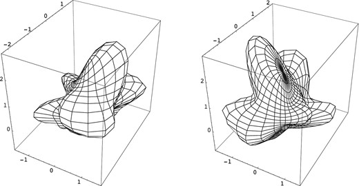
Views of grain 1 from two opposite directions.
GRS expansion coefficients. The full table is available online.
| Grain | l | m | alm | blm |
|---|---|---|---|---|
| 1 | 1 | 0 | 0.566 669 585 | −0.085 194 1355 |
| 1 | 1 | 1 | −0.367 041 01 | 0.213 834 444 |
| 1 | 2 | 0 | −0.053 580 3218 | −0.089 512 2548 |
| 1 | 2 | 1 | −0.005 563 869 57 | −0.008 703 381 94 |
| 1 | 2 | 2 | −0.066 820 0056 | 0.088 286 5188 |
| Grain | l | m | alm | blm |
|---|---|---|---|---|
| 1 | 1 | 0 | 0.566 669 585 | −0.085 194 1355 |
| 1 | 1 | 1 | −0.367 041 01 | 0.213 834 444 |
| 1 | 2 | 0 | −0.053 580 3218 | −0.089 512 2548 |
| 1 | 2 | 1 | −0.005 563 869 57 | −0.008 703 381 94 |
| 1 | 2 | 2 | −0.066 820 0056 | 0.088 286 5188 |
The derived quantities that characterize the 13 grains examined in this study are given in Tables 2 and 3.
GRS derived quantities.
| Grain | Va−3(1 + σ2)3/2 | rmax/aeff | |$S/(4 \pi a^2_{\mathrm{eff}})$| | |$\boldsymbol {r}_{\mathrm{cm}}/a_{\mathrm{eff}}$| | α1 | α2 | α3 |
|---|---|---|---|---|---|---|---|
| 1 | 10.568 | 2.2349 | 1.3430 | (0.289 92, −0.195 59, 0.504 64) | 1.7130 | 1.2900 | 1.0919 |
| 2 | 7.3329 | 2.4285 | 1.4011 | (0.024 61, 0.193 39, −0.449 91) | 2.1253 | 1.9392 | 0.811 56 |
| 3 | 8.7756 | 1.9046 | 1.2935 | (0.125 17, −0.313 83, 0.201 20) | 1.8185 | 1.5170 | 0.822 55 |
| 4 | 16.336 | 1.9635 | 1.2528 | (−0.595 78, −0.050 17, 0.198 73) | 1.9565 | 1.9084 | 0.690 20 |
| 5 | 6.8640 | 1.9173 | 1.2684 | (0.212 08, −0.325 22, −0.308 08) | 1.4298 | 1.3524 | 0.819 91 |
| 6 | 6.6200 | 2.1619 | 1.2632 | (−0.127 06, 0.463 37, 0.186 07) | 1.4923 | 1.3382 | 0.882 05 |
| 7 | 7.4806 | 2.2211 | 1.3596 | (0.082 03, −0.440 95, −0.126 76) | 1.8843 | 1.4960 | 0.897 30 |
| 8 | 7.4378 | 1.6693 | 1.1266 | (0.333 62, 0.184 62, −0.285 30) | 1.5227 | 1.1675 | 0.854 52 |
| 9 | 10.468 | 2.1160 | 1.1180 | (0.456 35, 0.097 77, −0.476 34) | 1.4005 | 1.2106 | 0.870 44 |
| 10 | 7.0687 | 1.8321 | 1.0893 | (−0.267 18, 0.170 87, 0.362 27) | 1.3109 | 1.1339 | 0.862 01 |
| 11 | 8.6542 | 1.9723 | 1.1240 | (0.139 15, 0.281 40, 0.487 41) | 1.4962 | 1.1479 | 0.878 68 |
| 12 | 12.710 | 2.1524 | 1.0968 | (−0.740 42, 0.259 73, 0.179 26) | 1.4447 | 1.3281 | 0.737 23 |
| 13 | 5.6324 | 1.5987 | 1.1207 | (0.026 09, −0.196 23, 0.086 27) | 1.5328 | 1.4072 | 0.722 68 |
GRS principal axes.
| Grain | |${\hat{\boldsymbol a}}_1$| | |${\hat{\boldsymbol a}}_2$| | |${\hat{\boldsymbol a}}_3$| |
|---|---|---|---|
| 1 | (0.865 99, −0.102 72, −0.489 39) | (0.498 15, 0.262 64, 0.826 36) | (0.043 66, −0.959 41, 0.278 61) |
| 2 | (0.473 29, 0.818 76, 0.325 01) | (0.831 96, −0.536 73, 0.140 58) | (0.289 54, 0.203 86, −0.935 20) |
| 3 | (0.663 04, −0.085 54, 0.743 68) | (0.745 08, 0.171 39, −0.644 57) | (−0.072 32, 0.981 48, 0.177 37) |
| 4 | (0.224 58, −0.271 27, −0.935 93) | (0.763 16, 0.646 20, −0.004 17) | (0.605 93, −0.713 33, 0.352 15) |
| 5 | (0.164 10, 0.698 32, −0.696 73) | (0.668 26, 0.440 84, 0.599 24) | (0.725 61, −0.563 93, −0.394 31) |
| 6 | (0.663 50, −0.353 68, 0.659 30) | (0.745 49, 0.237 98, −0.622 58) | (0.063 30, 0.904 58, 0.421 57) |
| 7 | (0.411 90, 0.056 21, −0.909 49) | (0.852 98, −0.374 91, 0.363 14) | (−0.320 56, −0.925 36, −0.202 37) |
| 8 | (0.297 77, 0.864 30, 0.405 35) | (0.475 72, 0.233 79, −0.847 96) | (−0.827 66, 0.445 33, −0.341 55) |
| 9 | (0.545 70, 0.832 19, −0.098 33) | (0.714 75, −0.400 99, 0.573 01) | (0.437 42, −0.382 97, −0.813 63) |
| 10 | (0.693 00, −0.720 83, 0.011 97) | (0.619 14, 0.603 58, 0.502 35) | (−0.369 33, −0.340 72, 0.864 58) |
| 11 | (0.947 10, 0.317 92, 0.043 84) | (0.018 55, −0.190 59, 0.981 49) | (0.320 39, −0.928 76, −0.186 41) |
| 12 | (0.497 03, −0.305 07, 0.812 34) | (0.600 56, 0.796 66, −0.068 27) | (−0.626 33, 0.521 79, 0.579 18) |
| 13 | (0.478 66, −0.353 95, −0.803 49) | (0.332 35, 0.920 09, −0.207 33) | (0.812 67, −0.167 80, 0.558 04) |
3 TORQUE CALCULATIONS: THEORY
3.1 Collisions of gas particles with the grain
A gas particle that approaches the grain and enclosing sphere along a radial path has θin = 0 and will hit the grain. A gas particle that approaches with θin = π/2 will not hit the grain. By construction, there is a unique distance from the origin to the grain surface for each direction (θ, ϕ). Thus, for each set of angles (θsph, ϕsph, ϕin), there is a critical value uc of cos θin such that a gas particle hits the grain when cos θin ≥ uc and does not hit when cos θin < uc. Our computational approach for determining uc as a function of (θsph, ϕsph, ϕin) is described in Section 4.1.
3.2 Torque due to incoming and reflected atoms
In this section, we calculate the torque due to gas particles (hereafter referred to as ‘atoms’, though the analysis is equally valid for molecules) that strike the grain, assuming that they stick to the grain or reflect specularly. In the next section, we will examine the torque associated with atoms or molecules that depart the grain after sticking to the surface.
We calculate the components of the mean torque along the |${\hat{\boldsymbol x}}$|, |${\hat{\boldsymbol y}}$|, and |${\hat{\boldsymbol z}}$| directions that are fixed relative to the grain body. Of course, these are identical to the components in an inertial frame with basis vectors that are instantaneously aligned with those of the grain frame. When these quantities are used to examine the grain rotational dynamics, they will be transformed to a single inertial frame and averaged over the grain rotation.
Now consider the case that atoms reflect specularly from the grain surface. Following a reflection, the atom may escape the grain or strike the grain surface at another location. In the latter case, the atom undergoes another specular reflection; this continues until the atom ultimately escapes the grain.
3.3 Mechanical torque due to outgoing atoms or molecules
We assume that the rate at which H atoms depart the grain (either in atomic form or as part of an H2 molecule) equals the rate at which they arrive at the grain. In this section, we consider only particles that stick to the grain surface upon arrival (as opposed to those that reflect specularly). We further assume that these outgoing particles depart along the direction |${\hat{\boldsymbol N}}(\theta , \phi )$| normal to the grain surface (see equation 14). In order to keep the computational time manageable, we do not consider a distribution of outgoing directions for atoms/molecules that have been accommodated on the grain surface. We consider the following scenarios for the departing particles.
(1) Atoms or molecules depart from an arbitrary location on the grain surface. The rate of departure from a surface element is proportional to its area.
(2) Atoms or molecules depart from approximately the same location where they arrived on the grain surface.
In future work we will also examine the case that molecules depart from a set of special sites of molecule formation on the grain surface.
3.4 Total mechanical torque
3.5 Rotational averaging
We assume that the grain rotates steadily about |${\hat{\boldsymbol a}}_1$|, as is appropriate for suprathermal rotation, and average the torque efficiency factors over this rotation.
It is convenient to express the averaged torque components in terms of spherical unit vectors |${\hat{\boldsymbol a}}_1$|, |${\hat{\boldsymbol \theta }}_v = {\hat{\boldsymbol x}}_v \cos \theta _{va} - {\hat{\boldsymbol z}}_v \sin \theta _{va}$|, and |${\hat{\boldsymbol \phi }}_v = {\hat{\boldsymbol y}}_v$|.
3.6 Drag torque
A rotating grain experiences a drag torque. Only the outgoing particles (reflected or otherwise) contribute since the angular momenta of the incoming atoms (as observed in an inertial frame) are not affected by the grain rotation. In scenarios (1) and (2), the outgoing particle departs along the local surface normal |${\hat{\boldsymbol N}}$|. After some number of times intersecting the grain surface (possibly zero), the particle's path along the local |${\hat{\boldsymbol N}}$| leads it to escape the grain. The outgoing particle's velocity in the torque expressions is |$v_{\mathrm{out}} {\hat{\boldsymbol N}}$|. For a rotating grain, this velocity is replaced with |$v_{\mathrm{out}} {\hat{\boldsymbol N}} + {\boldsymbol v}_{\mathrm{surf}}$|, where |${\boldsymbol v}_{\mathrm{surf}} = \omega \times (\boldsymbol {r}_{\mathrm{surf}} - \boldsymbol {r}_{\mathrm{cm}})$| is the velocity of the surface element due to the grain rotation. Thus, the expressions for the drag torque efficiency factors are identical to those for the mechanical torque except that |$v_{\mathrm{out}} {\hat{\boldsymbol N}}$| is replaced with |${\boldsymbol v}_{\mathrm{surf}}$|.
Since the orientation (θgr, ϕgr) of a rotating grain relative to the direction of the drift velocity is not constant, the drag torque efficiency factors must be averaged over the rotation. For steady rotation about |${\hat{\boldsymbol a}}_1$|, this is done as described in Section 3.5.
Since the motion of the grain can be neglected during the time interval that an outgoing particle is in the grain vicinity and the outgoing particle is always assumed to travel along |${\hat{\boldsymbol N}}$| in scenarios (1) and (2), the details of whether and where an outgoing particle strikes the grain surface are unaffected by the grain rotation. However, the velocity vector of the reflected particle does depend on rotation in the case of specular reflection, since the law of reflection applies in the rest frame of the surface element. This would introduce a major computational burden, since the particle paths would have to be traced anew for each value of the angular velocity. Thus, we do not compute the drag torque for the case of specular reflection.
In the case of a spherical grain at rest relative to the gas, uc = 0, rsph = aeff, |$\boldsymbol {r}_{\mathrm{cm}} = 0$|, sd = 0, and equation (74) simply evaluates to |$\boldsymbol {Q}_{\Gamma , \mathrm{drag, \, out}, (2)} = - 4 \pi ^{1/2} {\hat{\boldsymbol a}}_1 /3$|, which is a well-known result (see e.g. Draine & Weingartner 1996).
3.7 Extreme subsonic limit
As a check of our computer codes, we implement equations (79), (A11), and (84) to compute |$Q^{\prime }_{\mathrm{arr}}$|, |$\boldsymbol {Q}_{\Gamma , \mathrm{arr}}(s_{\rm d} = 0)$|, and |$\boldsymbol {Q}_{\Gamma , \mathrm{spec}}(s_{\rm d} = 0)$| and verify that they tend to zero as the numerical resolution improves.
3.8 Extreme supersonic limit
3.9 Mechanical/drag force
Of course, collisions with gas atoms give rise to a force as well as a torque on a grain. Although the grain rotational dynamics is our primary concern, for completeness and code verification purposes we provide expressions for the force in this section.
4 TORQUE CALCULATIONS: COMPUTATIONAL APPROACH
4.1 Incoming trajectories
We take the radius rsph of the enclosing sphere to be 1.01 rmax. (See the text following equation 19 for the definition of rmax.)
4.2 Arrival at the grain surface and reflection
Given uc as a function of (θsph, ϕsph, ϕin), we next examine trajectories for (θsph, ϕsph, ϕin, θin), with N1 + 1 values of θin spaced evenly in cos θin ∈ [uc, 1]. For each incoming trajectory, we tabulate the values of |$- {\hat{\boldsymbol s}}$| and |$({\hat{\boldsymbol r}} - \boldsymbol {r}_{\mathrm{cm}}/r_{\mathrm{sph}}) \times {\hat{\boldsymbol s}}$| for use in evaluating |$\boldsymbol {Q}_{F, \mathrm{arr}}$| and |$\boldsymbol {Q}_{\Gamma , \mathrm{arr}}$| (equations 100 and 38).
Next, we determine where the trajectory strikes the grain surface. Starting with the incoming particle's position and velocity on the enclosing sphere (as described in Section 4.1), we advance the particle along its trajectory, in steps of length 10−3rsph, until the particle reaches the grain interior. The final and penultimate steps bracket the intersection of the trajectory with the grain surface. The intersection point is then accurately found by 10 repeated bisections of this bracketing interval. This trajectory-tracing algorithm is not employed for the cases where cos θin = uc (since the arrival location on the grain surface was obtained when uc was determined) and cos θin = 1 [since the trajectory is radial in this case, it reaches the surface at (θ, ϕ) = (θsph, ϕsph)].
4.3 Integrals over the reduced speed
Prior to computing torques, we generate, using mathematica, interpolation tables for the function Is(p, sd, β) defined in equation (31) with 20 001 values of β for the value of sd under consideration and p = 3 and 4.
4.4 Characterization of the grain surface
We divide the grain surface into N2 × N2 patches, evenly spaced in cos θ and ϕ. Using the approach described in Section 4.2, we follow the trajectory of a particle departing the surface along the normal vector at the centre of each patch. We record whether or not the departing particle escapes to infinity or strikes the grain elsewhere (κesc = 1 or 0). If it escapes, then we record the vectors |${\hat{\boldsymbol N}}$|, |$\boldsymbol {r}_{\mathrm{surf}}$|, and |$(\boldsymbol {r}_{\mathrm{surf}} - \boldsymbol {r}_{\mathrm{cm}})/a_{\mathrm{eff}}$| for use in evaluating the force and torque associated with outgoing particles. If the departing particle strikes the grain elsewhere, then we record the index values of the patch that it strikes.
4.5 Torque evaluations
With the computational results from the preceding sections in hand, it is now straightforward to evaluate all of the efficiency factors. For outgoing scenario (2), we take the departure point for the outgoing particle to be the centre of the surface patch in which the incoming particle arrived. Similarly, when an outgoing particle strikes the grain surface elsewhere, we assume that the particle immediately departs along the surface normal in the centre of the patch that was struck.
We compute torques for (N3 + 1, N3) values of (θgr, ϕgr) and average over N3 values of Φ2 (when averaging over rotation about |${\hat{\boldsymbol a}}_1$|). For Qarr, |$\boldsymbol {Q}_{\Gamma , \mathrm{arr}}$|, |$\boldsymbol {Q}_{\Gamma , \mathrm{spec}}$|, |$\boldsymbol {Q}_{F, \mathrm{arr}}$|, |$\boldsymbol {Q}_{F, \mathrm{spec}}$|, |$\boldsymbol {Q}_{\Gamma , \mathrm{spec}}(s_{\rm d}=0)$|, |$\boldsymbol {Q}^{\prime }_{\Gamma , \mathrm{spec}}$|, |$\boldsymbol {Q}_{F, \mathrm{spec}}(s_{\rm d}=0)$|, |$\boldsymbol {Q}^{\prime }_{F, \mathrm{spec}}$|, |$\boldsymbol {Q}_{\Gamma , \mathrm{out}, (2)}$|, |$\boldsymbol {Q}_{F, \mathrm{out}, (2)}$|, |$\boldsymbol {Q}_{\Gamma , \mathrm{out}, (2)}(s_{\rm d} = 0)$|, |$\boldsymbol {Q}^{\prime }_{\Gamma , \mathrm{out}, (2)}$|, |$\boldsymbol {Q}_{\Gamma , \mathrm{drag, \, out}, (2)}(s_{\rm d} = 0)$|, and |$\boldsymbol {Q}^{\prime }_{\Gamma , \mathrm{drag, \, out}, (2)}$|, integrals are evaluated with (N1 + 1, N1, N1, N1 + 1) values of (θsph, ϕsph, ϕin, θin). For Qarr(sd = 0), |$Q^{\prime }_{\mathrm{arr}}$|, |$\boldsymbol {Q}_{\Gamma , \mathrm{arr}}(s_{\rm d}=0)$|, |$\boldsymbol {Q}^{\prime }_{\Gamma , \mathrm{arr}}$|, |$\boldsymbol {Q}_{F, \mathrm{arr}}(s_{\rm d}=0)$|, and |$\boldsymbol {Q}^{\prime }_{F, \mathrm{arr}}$|, integrals are evaluated with (N1 + 1, N1, N1) values of (θsph, ϕsph, ϕin). Integrals for |$\boldsymbol {Q}_{\Gamma , \mathrm{out}, (1)}/Q_{\mathrm{arr}}$|, |$\boldsymbol {Q}_{\Gamma , \mathrm{drag, \, out}, (1)}/Q_{\mathrm{arr}}$|, and |$\boldsymbol {Q}_{F, \mathrm{out}, (1)}/Q_{\mathrm{arr}}$| are evaluated with (4096, 4096) values of (θsurf, ϕsurf).
For the efficiency factors in the extreme supersonic limit, we first evaluate μhit for (N1 + 1, N1, N3 + 1, N3) values of (θ, ϕ, θgr, ϕgr). We employ the trajectory-tracing algorithm described in Section 4.2, except that we start at location (θ, ϕ) on the surface and move outwards along |${\hat{\boldsymbol N}}(\theta , \phi )$| to determine whether or not (θ, ϕ) is shadowed by another part of the grain. The integrals in equations (93) and (95–98) are then easily evaluated.
4.6 Code verification: spherical grains
Our codes reproduce all of these results for a spherical grain, for which all of the GRS expansion coefficients alm and blm vanish. We tested for numerous combinations of (θgr, ϕgr), in the extreme subsonic and supersonic limits and with sd = 1.
5 TORQUE CALCULATIONS: COMPUTATIONAL RESULTS
5.1 Arrival rate and torques
In this section, we present computational results for grain 1.
In order to check for convergence of the numerical integrals that appear in the expressions for the efficiency factors, we first construct a table of data used in computing the integrands with N1 = 27 = 128. Recall that there are N1 values of ϕsph and ϕin and N1 + 1 values of cos θsph and cos θin. Since N1 is a power of 2, the tabulated data can be used to evaluate the integrals with N1 = 16, 32, 64, and 128. We find that 64 is often sufficient, though 128 is sometimes required. For sd = 10, even N1 = 128 is not sufficient for full convergence. For efficiency factors associated with outgoing particles, we typically adopt N2 = 256 (recall that we divide the surface into |$N_2^2$| patches when examining the trajectories of outgoing particles). We also ran some computations with N2 = 128 and 512 to check for convergence in this parameter. The number of orientations (θgr, ϕgr) (of the grain body relative to the drift velocity) for which quantities are computed affects the convergence of the rotationally averaged values. We have tried N3 = 32, 64, and 128 (as well as 256 in the case of the supersonic limit).
Fig. 2 shows |$\overline{Q}_{\mathrm{arr}}$| for various values of sd; from equation (78), Qarr(sd = 0) = 4.57. The dashed curves in Fig. 2 are for the extreme supersonic limit, scaled to sd = 3 and 10. Recall that, for the subsonic limit, the first-order dependence on sd (|$Q^{\prime }_{\mathrm{arr}}$|) vanishes. Since |${\hat{\boldsymbol a}}_1$| is the principal axis of greatest moment of inertia, the grain presents its largest cross-sectional area to the flowing gas when |${\hat{\boldsymbol a}}_1$| lies along the velocity vector. This explains the dependence of |$\overline{Q}_{\mathrm{arr}}$| on cos θva, which is most pronounced in the supersonic limit.
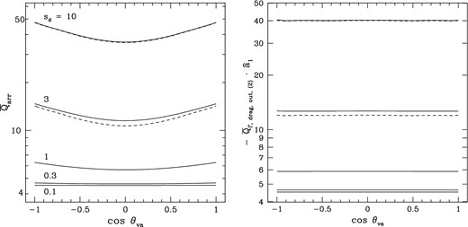
Left: the grain 1 efficiency factor |$\overline{Q}_{\mathrm{arr}}$| for the rate at which gas atoms arrive at the grain surface, averaged over rotation about |${\hat{\boldsymbol a}}_1$|, as a function of the angle θva between |${\hat{\boldsymbol a}}_1$| and the grain velocity for various values of the reduced grain drift speed sd. Right: the drag torque efficiency factor |$\boldsymbol {Q}_{\Gamma , \mathrm{drag, \, out}, (2)}$| (component along |${\hat{\boldsymbol a}}_1$|) for the same values of sd (higher curves are for higher sd). In both cases, dashed curves are the result for the extreme supersonic limit, scaled to sd = 3 and 10.
Figs 3 –5 show the components of the rotationally averaged efficiency factor for the torque due to arriving atoms (|$\overline{\boldsymbol {Q}}_{\Gamma , \mathrm{arr}}$|), specular reflection (|$\overline{\boldsymbol {Q}}_{\Gamma , \mathrm{spec}}$|), and outgoing scenario 2 (|$\overline{\boldsymbol {Q}}_{\Gamma , \mathrm{out, (2)}}$|), along |${\hat{\boldsymbol a}}_1$|, |${\hat{\boldsymbol \theta }}_v$|, and |${\hat{\boldsymbol \phi }}_v$| (defined in the last sentence in Section 3.5). In the absence of an interstellar magnetic field, these components drive rotation about |${\hat{\boldsymbol a}}_1$|, alignment of |${\hat{\boldsymbol a}}_1$| with respect to the direction |${\hat{\boldsymbol s}}_{\rm d}$| of the grain drift, and precession of |${\hat{\boldsymbol a}}_1$| about |${\hat{\boldsymbol s}}_{\rm d}$|. The solid curves are results for sd = 0.1, 0.3, 1.0, 3.0, and 10.0. Results computed in the extreme subsonic limit and scaled to sd = 0.1, 0.3, and 1.0 are displayed as long-dashed curves. Similarly, results computed in the extreme supersonic limit and scaled to sd = 1.0, 3.0, and 10.0 are displayed as short-dashed curves.
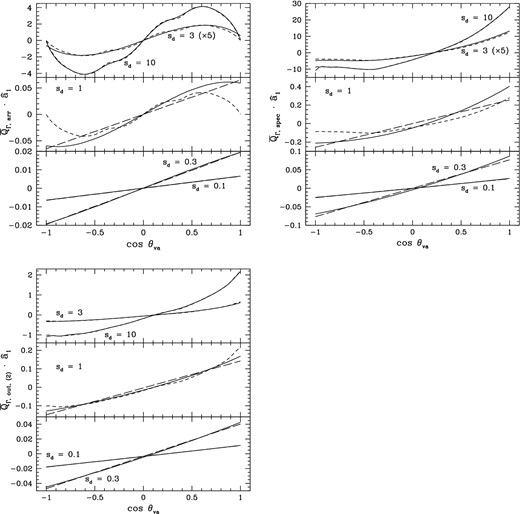
Rotationally averaged grain 1 efficiency factor for the torque component along |${\hat{\boldsymbol a}}_1$| due to the arrival of gas atoms (|$\overline{\boldsymbol {Q}}_{\Gamma , \mathrm{arr}}$|), specular reflection (|$\overline{\boldsymbol {Q}}_{\Gamma , \mathrm{spec}}$|), and outgoing scenario 2 (|$\overline{\boldsymbol {Q}}_{\Gamma , \mathrm{out, (2)}}$|). The lower, middle, and upper subpanels are for sd = (0.1, 0.3), 1.0, and (3.0, 10.0), respectively. Long-dashed (short-dashed) curves are results for the extreme supersonic (subsonic) limits, scaled to the corresponding value of sd.
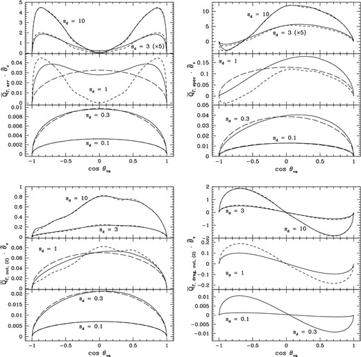
Same as Fig. 3, except for the component along |${\hat{\boldsymbol \theta }}_v$| and including the drag torque efficiency |$\boldsymbol {Q}_{\Gamma , \mathrm{drag, \, out}, (2)}$|.
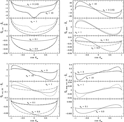
Same as Fig. 4, except for the component along |${\hat{\boldsymbol \phi }}_v$|.
As seen in Figs 2–5, results associated with arriving atoms for sd = 0.1 and 0.3 agree very well with those for the subsonic limit and results for sd = 3 and 10 agree very well with those for the supersonic limit. Different computer codes are used for computing results in the cases of a specified value of sd, the extreme subsonic limit, and the extreme supersonic limit. As described in the previous sections, the algorithm for the subsonic (supersonic) limit is somewhat (very) different from that for a specified sd. Thus, the agreement of the results is confirmation of the validity of the codes.
The following features of |$\overline{\boldsymbol {Q}}_{\Gamma , \mathrm{arr}}$| exhibited in Figs 3 and 4 are worth noting: 1. |$\overline{\boldsymbol {Q}}_{\Gamma , \mathrm{arr}} {\cdot } {\hat{\boldsymbol a}}_1$| is an odd function of cos θva and is proportional to cos θva for subsonic drift, 2. |$\overline{\boldsymbol {Q}}_{\Gamma , \mathrm{arr}} {\cdot } {\hat{\boldsymbol \theta }}_v$| is an even function of cos θva and is proportional to sin θva for subsonic drift, 3. |$\overline{\boldsymbol {Q}}_{\Gamma , \mathrm{arr}} {\cdot } {\hat{\boldsymbol a}}_1$| and |$\overline{\boldsymbol {Q}}_{\Gamma , \mathrm{arr}} {\cdot } {\hat{\boldsymbol \theta }}_v$| have the same sign when cos θva > 0, 4. |$\overline{\boldsymbol {Q}}_{\Gamma , \mathrm{arr}} {\cdot } {\hat{\boldsymbol \theta }}_v (\cos \theta _{va} = 0) \rightarrow 0$| as sd → ∞, 5. |$\overline{\boldsymbol {Q}}_{\Gamma , \mathrm{arr}} {\cdot } {\hat{\boldsymbol a}}_1 (\cos \theta _{va} = \pm 1) \rightarrow 0$| as sd → ∞, 6. |$\overline{\boldsymbol {Q}}_{\Gamma , \mathrm{arr}} {\cdot } {\hat{\boldsymbol \theta }}_v (\cos \theta _{va} = \pm 1) = 0$|. As shown in Appendix B, these properties are satisfied for all grain shapes. Our computational results exhibit most of these features for all 13 grains, providing further evidence that the code is robust. There are slight deviations from the expected form for |$\overline{\boldsymbol {Q}}_{\Gamma , \mathrm{arr}} {\cdot } {\hat{\boldsymbol \theta }}_v$| in the subsonic regime for grains 3, 10, and 11, and somewhat larger deviations for grains 5 and 9, suggesting that the computations are not fully converged in these cases. In addition, the computational result for |$\overline{\boldsymbol {Q}}_{\Gamma , \mathrm{arr}} {\cdot } {\hat{\boldsymbol a}}_1$| is always slightly offset in cos θva; i.e. it passes through zero at a value of cos θva slightly different from zero.
In producing the curves in Figs 2–5, we adopted N1 = 128 for sd = 0.1–3.0 and N1 = 256 for sd = 10. Given the close agreement between the results for sd = 10 with the supersonic results scaled to sd = 10, we will simply adopt the latter for grains 2–13. This greatly reduces the computational time.
Appendix C notes some features that characterize all of the rotationally averaged torque efficiencies in the extreme subsonic limit. We have verified that our results display these features for all 13 grain shapes.
Fig. 2 also displays the |${\hat{\boldsymbol a}}_1$|-component of the rotationally averaged drag torque efficiency factor |$\overline{\boldsymbol {Q}}_{\Gamma , \mathrm{drag, \, out}, (2)}$| computed for outgoing scenario (2). These results agree well with those computed in the extreme supersonic limit and scaled to sd = 3 and 10. In the limit of low sd, the results tend towards that found for sd = 0: |$\boldsymbol {Q}_{\Gamma , \mathrm{drag, \, out}, (2)} {\cdot } {\hat{\boldsymbol a}}_1 = -4.51$|. We found an extremely weak first-order dependence of |$\boldsymbol {Q}_{\Gamma , \mathrm{drag, \, out}, (2)}$| on sd; i.e. |$\boldsymbol {Q}^{\prime }_{\Gamma , \mathrm{drag, \, out}, (2)} {\cdot } {\hat{\boldsymbol a}}_1 \ll 1$| (and likewise for the other components). We computed the second-order term and found that its inclusion substantially overestimates QΓ, drag, out, (2) for small sd. Evidently a power-series expansion converges slowly in the low-sd limit. Figs 4 and 5 display |${\hat{\boldsymbol \theta }}_v$|- and |${\hat{\boldsymbol \phi }}_v$|-components of |$\overline{\boldsymbol {Q}}_{\Gamma , \mathrm{drag, \, out}, (2)}$|. Curves for the subsonic limit are not displayed because of the poor convergence behaviour.
For grains 2–13, plots of the rotationally averaged arrival efficiency |$\overline{Q}_{\mathrm{arr}}$| versus cos θva look very similar to that for grain 1, but with somewhat smaller magnitudes when α = 3 than when α = 2. Plots of the various torque efficiencies versus cos θva generally show a wide diversity of shapes, again with the magnitudes often smaller when α = 3 than when α = 2. The components of the drag torque efficiency along |${\hat{\boldsymbol a}}_1$| and |${\hat{\boldsymbol \theta }}_v$| are broadly similar, but the component along |${\hat{\boldsymbol \phi }}_v$| varies considerably among the grain shapes.
In outgoing scenario (1), the torque and drag efficiencies are both proportional to the arrival efficiency Qarr. Since the angle θva does not change when the grain rotates around |${\hat{\boldsymbol a}}_1$|, |$\overline{Q}_{\mathrm{arr}}$| remains constant for this motion. Thus, the components of |$\overline{\boldsymbol {Q}}_{\Gamma , \mathrm{out}, (1)}$| and |$\overline{\boldsymbol {Q}}_{\Gamma , \mathrm{drag, out}, (1)}$| along |${\hat{\boldsymbol \theta }}_v$| and |${\hat{\boldsymbol \phi }}_v$| vanish. (We assume that the time when an atom or molecule departs the grain surface is uncorrelated with the arrival time of the atom.) The components of the drag efficiency along |${\hat{\boldsymbol a}}_1$| are given in Table 4. For most of the grain shapes, |$\boldsymbol {Q}_{\Gamma , \mathrm{out}, (1)} {\cdot } {\hat{\boldsymbol a}}_1 / Q_{\mathrm{arr}}$| is consistent with zero, having not converged when evaluated using (4096)2 patches on the surface. The exceptions are grain 4, for which |$\boldsymbol {Q}_{\Gamma , \mathrm{out}, (1)} {\cdot } {\hat{\boldsymbol a}}_1 / Q_{\mathrm{arr}} = 0.001\,22$|, and grains 2 and 3, for which |$\boldsymbol {Q}_{\Gamma , \mathrm{out}, (1)} {\cdot } {\hat{\boldsymbol a}}_1 / Q_{\mathrm{arr}}$| appears to converge to ∼ −3 × 10⁻⁵ and ∼6 × 10⁻⁶, respectively.
Drag efficiency factors in outgoing scenario (1).
| Grain index | |$\boldsymbol {Q}_{\Gamma , \mathrm{drag, out}, (1)} {\cdot } {\hat{\boldsymbol a}}_1 / Q_{\mathrm{arr}}$| |
|---|---|
| 1 | −0.979 |
| 2 | −1.091 |
| 3 | −1.004 |
| 4 | −1.052 |
| 5 | −0.821 |
| 6 | −0.888 |
| 7 | −1.054 |
| 8 | −0.904 |
| 9 | −0.864 |
| 10 | −0.819 |
| 11 | −0.911 |
| 12 | −0.873 |
| 13 | −0.907 |
5.2 Forces
As noted in Section 3.9, |$\boldsymbol {Q}_{F, \mathrm{arr}}$| and |$\boldsymbol {Q}_{F, \mathrm{spec}}$| both vanish when sd = 0. Thus, the force is entirely drag when fspec = 1. The component of the rotationally averaged drag force antiparallel to the grain's velocity is comparable in magnitude to that on a sphere (ranging between about 75 and 230 per cent of that for a sphere in all cases) but varies with θva, with its maximum value when cos θva = ±1 and minimum near cos θva = 0. There is also a component perpendicular to the grain's velocity which vanishes at cos θva = ±1 and near cos θva = 0 and can reach values as high as about 30 per cent of the drag force on a spherical grain.
For outgoing scenario (2), the force can be non-zero when sd = 0. However, we have found that this term does not contribute substantially even when sd = 0.1. The drag force in this case is qualitatively and quantitatively similar to that in the case of specular reflection.
For outgoing scenario (1), |$\boldsymbol {Q}_{F, \mathrm{out}, (1)}$| is proportional to Qarr and its direction is fixed in grain-body coordinates; only the component along |${\hat{\boldsymbol a}}_1$| is non-zero when averaged over the grain rotation. For most shapes, |$\boldsymbol {Q}_{F, \mathrm{out}, (1)} {\cdot } {\hat{\boldsymbol a}}_1 / Q_{\mathrm{arr}}$| is consistent with zero, having not converged when evaluated using (4096)2 patches on the surface. The exceptions are grains 3 and 4, for which |$\boldsymbol {Q}_{F, \mathrm{out}, (1)} {\cdot } {\hat{\boldsymbol a}}_1 / Q_{\mathrm{arr}} = 0.001\,28$| and −0.003 44, respectively, and grain 2, for which |$\boldsymbol {Q}_{F, \mathrm{out}, (1)} {\cdot } {\hat{\boldsymbol a}}_1 / Q_{\mathrm{arr}}$| appears to converge to ∼2 × 10⁻⁵. The drag force associated with the arriving atoms only is similar to that for the above cases, with a somewhat smaller range of magnitudes.
6 DYNAMICS
6.1 Equations of motion
6.2 Stationary points
6.3 Crossover points
6.4 Results
We have examined the grain rotational dynamics for sd = 0.1, 0.3, 1.0, 3.0, and 10.0. Table 5 gives the adopted values of the relevant parameters. The speed of the outgoing particle is vout = (2kTdust/mp)1/2 for H atoms (with Tdust the temperature of the grain) and vout = (EH2/mp)1/2 for H2 molecules.
Adopted parameter values for grain rotational dynamics.
| aeff | 0.2 μm |
| ρ | 3.0 g cm−3 |
| χ0 | 3.3 × 10⁻⁴ |
| B | 5.0 μG |
| Tdust | 15 K |
| Tgas | 100 K |
| EH2 | 0.2 eV |
| nH | 30 cm−1 |
| aeff | 0.2 μm |
| ρ | 3.0 g cm−3 |
| χ0 | 3.3 × 10⁻⁴ |
| B | 5.0 μG |
| Tdust | 15 K |
| Tgas | 100 K |
| EH2 | 0.2 eV |
| nH | 30 cm−1 |
Fig. 6 is a ‘trajectory map’, which shows how (cos ξ, ω′) evolves for grain 1 with sd = 0.1 when the outgoing particles are H atoms in scenario (2) and ψv = 89°. This map features an attractor at (cos ξ, ω′) = (1, −31.7), a repellor at (−1, −58.4), a crossover attractor at cos ξ = −1 and a crossover repellor at cos ξ = 1. Draine & Weingartner (1997) classified trajectory maps in three categories. This is an example of a non-cyclic map, in which all of the trajectories land on the attractor, and it exhibits perfect alignment with the magnetic field, since ξ = 0 for the attractor. The other categories are cyclic maps, which exhibit no attractors, so that the grain state must cycle between crossovers indefinitely, and semicyclic maps, for which the grain state may either land on an attractor or cycle between crossovers. Since our analysis assumes that the grain angular momentum always lies along |${\hat{\boldsymbol a}}_1$|, we cannot follow the dynamics through the crossovers and determine which of these possibilities actually occurs for semicyclic maps.
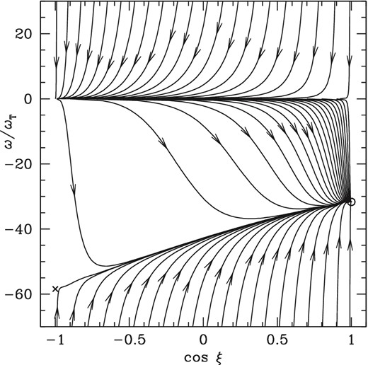
Trajectory map for grain 1, sd = 0.1, ψv = 89°, and atoms as the outgoing particles in scenario (2). The rotational speed ω is normalized to the thermal value ωT (equation 151); ξ is the alignment angle. The attractor (repeller) is indicated by the open circle (cross).
In future work, we will relax the assumption that the angular momentum always lies along |${\hat{\boldsymbol a}}_1$|, enabling a firm conclusion regarding the effectiveness of mechanical torques in aligning grains. Here we attempt to gain some insight by examining the incidence of attractors satisfying the following three conditions that are conducive to alignment: (1) |cos ξ| ≥ 1/3, ensuring that the ‘Rayleigh reduction factor’ characterizing the alignment effectiveness is positive (Lee & Draine 1985); (2) τalign ≤ 106 yr, in order to be competitive with radiative torques (Draine & Weingartner 1997); (3) ω/ωT ≥ 3, so as to avoid disalignment due to collisions with gas particles (Lazarian & Hoang 2007b; Hoang & Lazarian 2008). For each of the 13 grain shapes, five assumptions regarding the outgoing particles, and five values of sd, we consider 100 values of ψv between 0 and π/2, uniformly spaced in cos ψv. Fig. 7 shows fattract, the fraction of values of ψv for which the trajectory map contains one or more attractors (making it non-cyclic or semicyclic) satisfying the above three conditions.
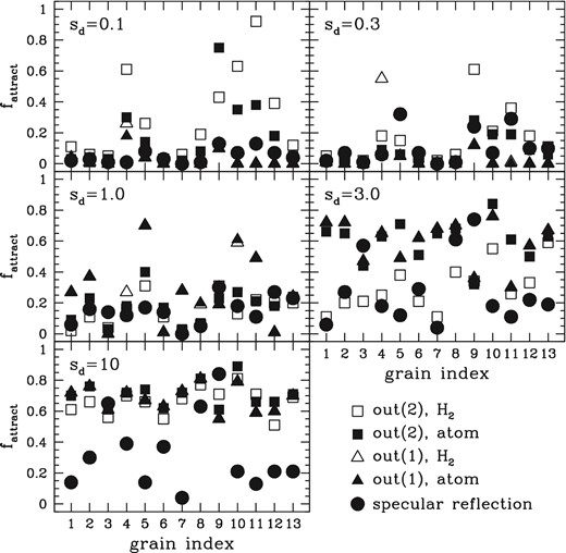
For each of 65 cases (13 grain shapes and five assumptions regarding outgoing particles) and with five values of sd as indicated in each panel, the fraction fattract of values of ψv (uniformly distributed in cos ψv) for which the trajectory map contains one or more attractors satisfying the alignment-conducive conditions described in the text.
With the exception of grain 4, we include only the torque associated with the arriving atoms in the case of outgoing scenario (1), since |$\boldsymbol {Q}_{\Gamma , \mathrm{out}, (1)} {\cdot } {\hat{\boldsymbol a}}_1 / Q_{\mathrm{arr}}$| is consistent with zero for most of the shapes. Thus, except for grain 4, the open and filled triangles are coincident in Fig. 7. As noted in Section 5.1, |$\boldsymbol {Q}_{\Gamma , \mathrm{out}, (1)} {\cdot } {\hat{\boldsymbol a}}_1 / Q_{\mathrm{arr}}$| appears to converge to a small but non-zero value for grains 2 and 3. Including the associated torque does not alter the value of fattract in any case for grain 3, but does alter its value for grain 2 by ±0.01 in some cases.
The fraction fattract varies considerably depending on grain shape, outgoing particle characteristics, and sd. On the whole, fattract is larger for supersonic drift than for subsonic drift, suggesting more effective alignment in the former case. This may be partially offset by the result that maps with attractors tend to be non-cyclic in cases of subsonic drift and semicyclic in cases of supersonic drift (except that semicyclic character always dominates in the case of specular reflection). Even for subsonic drift, fattract can approach unity for some grain shapes and outgoing scenarios. Thus, the simple analysis assuming that |$\boldsymbol {J} \parallel {\hat{\boldsymbol a}}_1$| indicates that alignment via mechanical torques may be viable for both subsonic and supersonic drift; a more detailed study that relaxes this assumption is needed.
6.5 Analysis
We have found that the increase in fattract with sd is commonly due to an increase in the number of attractors as sd increases rather than an increase in the fraction of attractors that satisfy the three imposed conditions. To gain some insight into this observation, consider how the overall magnitudes and the shapes of the torques (i.e. plots of the rotationally averaged efficiency factor components as functions of cos θva) vary with sd and how these affect the incidence of attractors and the associated values of ω/ωT and τalign.
Denote the overall magnitudes of the mechanical and drag torque efficiencies by |$\tilde{Q}_{\Gamma , \mathrm{mech}}$| and |$\tilde{Q}_{\Gamma , \mathrm{drag}}$|, respectively. Both of these tend to increase with sd. As noted in Section 3.8, in the extreme supersonic limit, the torques associated with arriving atoms and specular reflection increase in proportion to |$s_{\rm d}^2$| and the outgoing-particle and drag torques increase in proportion to sd. In the subsonic limit (Section 3.7), |$\boldsymbol {Q}_{\Gamma , \mathrm{arr}} \propto s_{\rm d}$|. The other mechanical torques can be non-vanishing when sd = 0; thus, their overall magnitude does not necessarily increase monotonically with sd in the subsonic limit (though this happens to be the case for grain 1). As seen in Fig. 2 (recall that |$\boldsymbol {Q}_{\Gamma , \mathrm{drag, out, (1)}} \propto Q_{\mathrm{arr}}$|), |$\tilde{Q}_{\Gamma , \mathrm{drag}}$| increases very slowly with sd in the subsonic limit and |$\tilde{Q}_{\Gamma , \mathrm{drag}} \propto s_{\rm d}$| in the supersonic limit.
If only the arriving atoms contributed to the mechanical torque, then its shape would not depend on sd in either the extreme subsonic or supersonic limits, though it would depend on sd for intermediate values of sd. The shape of the total mechanical torque can vary in all of the regimes that we examine since it is the sum of two terms (arrival plus specular reflection or outgoing scenario 1 or 2) that vary with sd in different ways. (Of course, for sufficiently large sd, the shape does not depend on sd, but at sd = 10 the magnitude of |$\overline{\boldsymbol {Q}}_{\Gamma , \mathrm{arr}}$| does not yet overwhelm that of |$\overline{\boldsymbol {Q}}_{\Gamma , \mathrm{out}}$|. Also, the shapes of |$\overline{\boldsymbol {Q}}_{\Gamma , \mathrm{spec}}$| and |$\overline{\boldsymbol {Q}}_{\Gamma , \mathrm{out}}$| individually can vary with sd at low sd since they do not necessarily vanish when sd = 0.) The shape of the drag torque also varies with sd, but we have found that the dynamics is not greatly modified if the drag components perpendicular to |${\hat{\boldsymbol a}}_1$| are ignored. Furthermore, the variation of |$\overline{\boldsymbol {Q}}_{\Gamma , \mathrm{drag, out}, (2)} \cdot {\hat{\boldsymbol a}}_1$| with θva is mild.
Now consider how the various quantities that affect the dynamics depend on |$\tilde{Q}_{\Gamma , \mathrm{mech}}$| and |$\tilde{Q}_{\Gamma , \mathrm{drag}}$|: Jv and Hv are both proportional to |$\tilde{Q}_{\Gamma , \mathrm{mech}}$|, τdrag and Mv are both proportional to |$\tilde{Q}^{-1}_{\Gamma , \mathrm{drag}}$|, and Jdrag and Hdrag are both independent of the overall torque magnitudes.
Thus, the function Zv(ξ) (equation 156) is proportional to |$\tilde{Q}_{\Gamma , \mathrm{mech}}$|. Since stationary points are located at ξ for which Zv(ξ) = 0, the incidence of stationary points depends only on the shapes of the torques, not on their overall magnitudes. We have found that the great majority of the attractors lie at ξ = 0 or π, where stationary points are always located. Since the suprathermality |$\omega ^{\prime }_s \propto \tilde{Q}_{\Gamma , \mathrm{mech}} / \tilde{Q}_{\Gamma , \mathrm{drag}}$|, it tends to increase with sd and approaches values as large as 105 in some cases when sd = 10.
The terms Al and Dl that appear in the linearized dynamical equations (equations 158–163) are independent of the overall torque magnitudes while |$B_l \propto \tilde{Q}_{\Gamma , \mathrm{drag}} \tilde{Q}^{-1}_{\Gamma , \mathrm{mech}}$| and |$C_l \propto \tilde{Q}_{\Gamma , \mathrm{mech}} \tilde{Q}^{-1}_{\Gamma , \mathrm{drag}}$|. Thus, the conditions for a stationary point to be an attractor (equation 165) are independent of the overall torque magnitude. The increase in the number of attractors with sd must result from the change in the shape of the mechanical torque as sd increases.
Since the denominator in the expression for τalign in equation (166) does not depend on the overall torque magnitudes, the alignment time varies with sd in exactly the same way as the drag time, namely in proportion to |$\tilde{Q}^{-1}_{\Gamma , \mathrm{drag}}$|. Thus, the distribution of alignment times does not vary substantially as sd increases through the subsonic regime but does decrease with sd in the supersonic regime.
Now we will apply the above observations to the dynamics in the case of outgoing scenario (1). Except for grain 4, the torque associated with the outgoing atoms/molecules is negligible compared with the torque associated with the incoming atoms in this scenario. Thus, |$Q_{a1}(\cos \theta _{va}) = \overline{\boldsymbol {Q}}_{\Gamma , \mathrm{arr}}(\cos \theta _{va}) {\cdot } {\hat{\boldsymbol a}}_1$| and |$Q_{\theta }(\cos \theta _{va}) = \overline{\boldsymbol {Q}}_{\Gamma , \mathrm{arr}}(\cos \theta _{va}) {\cdot } {\hat{\boldsymbol \theta }}_v$|. The incidence of attractors at ξ = 0 or π as a function of sd can be explained from the grain-shape-independent properties of Qa1 and Qθ derived in Appendix B. (For the remainder of this discussion, it will be implicit that the attractors under discussion lie at ξ = 0 or π.)
First, since Qa1(0) = 0, no attractors with suprathermal rotation are expected for cos ψv = 0. Secondly, when cos ψv = ±1, the condition for an attractor is that Al given by equation (171) must be less than zero. Since Qa1 and Qθ have the same sign when cos θva > 0 and Qθ(cos θva = ±1) = 0, dQθ/dθva has the same sign as Qa1 for the stationary point at ξ = 0. Thus, Al > 0 and this point is not an attractor. A similar analysis shows that the stationary point at ξ = π is also not an attractor.
As seen in Fig. 7, our computed fattract for outgoing scenario (1) does not equal zero in the subsonic regime for grains 2, 5, and 9. For grain 2, this occurs because the computational result for Qa1(cos θva) crosses zero at cos θva ≈ −0.018 rather than at zero. As a result, Qa1 has the wrong sign for a small range of cos θva, yielding spurious attractors at ξ = π for ψv very close to 90°. Although this slight offset in Qa1(cos θva) afflicts the computational results for all grains, it is only large enough to affect fattract for grain 2. For grains 5 and 9, deviations of the shape of the computed Qθ(cos θva) from sin θva are responsible for the spurious attractors. We have generated a version of Fig. 7 for the subsonic regime using torques computed with N1 = 64 rather than 128. (Recall that there are N1 values of ϕsph and ϕin and N1 + 1 values of cos θsph and cos θin.) With N1 = 64, fattract for outgoing scenario (1) is somewhat higher for grains 2, 5, and 9 and also non-zero for grains 3, 6, 10, and 11. Thus, fattract approaches zero as the numerical resolution increases, in agreement with our idealized model.
In the case of grain 4, |$\boldsymbol {Q}_{\Gamma , \mathrm{out}, (1)} {\cdot } {\hat{\boldsymbol a}}_1$| is not negligible. For sd = 0.1, |$\overline{\boldsymbol {Q}}_{\Gamma , \mathrm{arr}} {\cdot } {\hat{\boldsymbol a}_1} \approx -7 \times 10^{-3} \cos \theta _{va}$|, |$\boldsymbol {Q}_{\Gamma , \mathrm{out}, (1)} {\cdot } {\hat{\boldsymbol a}}_1 / Q_{\mathrm{arr}} = 0.001\,22$|, and Qarr ≈ 4.3. Evaluating vout/vth for the cases of atomic and molecular outgoing particles using the parameter values in Table 5, we find that Qa1 ≈ Q0 − 7 × 10⁻³cos θva with Q0 ≈ 1.9 × 10⁻³ for atoms and Q0 ≈ 1.7 × 10⁻² for molecules. Due to the upward shift of Qa1, Qa1 and Qθ have opposite signs when 0 < cos θva < 0.28 for atoms and when 0 < cos θva < 1 for molecules. Thus, attractors arise at ξ = 0 for cos ψv between 0 and 0.28 (0 and 1) for atomic (molecular) outgoing particles. Since these attractors do not all satisfy the conditions on ω′ and τalign for effective alignment, fattract is less than 0.28 and 1 in these cases. A similar analysis applies when sd = 0.3. Thus, it appears that subsonic mechanical torques can yield effective alignment even in the case of outgoing scenario (2) if the grain shape is such that |$\boldsymbol {Q}_{\Gamma , \mathrm{out}, (1)} {\cdot } {\hat{\boldsymbol a}}_1$| is not negligible, but that such shapes are rare. Of course, we are unable to draw a strong conclusion on this point since we have only examined 13 shapes.
The upper panel in Fig. 8 shows fattract versus fattract, max for sd = 0.1 for all 13 grain shapes, considering specular reflection and both outgoing scenarios. In most cases, fattract < fattract, max, commonly because τalign > 106 yr for the attractors. In cases where fattract > fattract, max, the simplifying assumptions may be violated or there may be error due to insufficient numerical resolution in the torque evaluations.
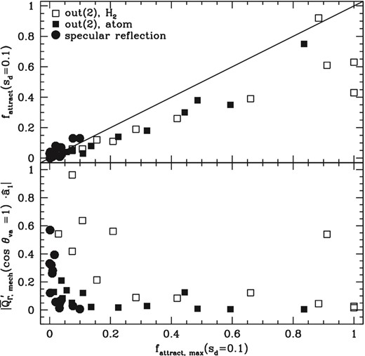
fattract (upper panel) and |$|\overline{\boldsymbol {Q}}^{ \prime }_{\Gamma , \mathrm{mech}}(\cos \theta _{va} =1) \cdot {\hat{\boldsymbol a}}_1|$| (lower panel) versus fattract, max for sd = 0.1
The lower panel in Fig. 8 shows |$|\overline{\boldsymbol {Q}}^{ \prime }_{\Gamma , \mathrm{mech}}(\cos \theta _{va} =1) \cdot {\hat{\boldsymbol a}}_1|$|, a measure of the overall magnitude of the mechanical torque, again for sd = 0.1. Note that, typically, the cases for which fattract is substantial are characterized by low torque magnitudes. This is expected from the above analysis: the mechanical torque in the subsonic regime is the sum of a constant term that persists when sd = 0 and a term proportional to sd. The larger the former is in comparison to the latter, the larger the range of cos ψv for which attractors can occur. The one case for which both fattract and the torque magnitude are large is for H2 molecules departing in scenario (2) from grain 4. As with outgoing scenario (1), this grain happens to experience an unusually large torque even when not drifting relative to the gas.
As seen in Fig. 7, for some of the cases with relatively large fattract when sd = 0, fattract is lower when sd = 0.3; the term that persists when sd = 0 is relatively less important when sd = 0.3 than when sd = 0.1. As discussed earlier, the increase in fattract as sd increases beyond 1 is due to the change in the shape of the torques; the torque that persists for zero drift is unimportant in these cases.
These results suggest that grain shapes which are most susceptible to alignment by mechanical torques in the subsonic regime may typically experience relatively weak mechanical torques, which therefore are more likely to be dominated by other types of torques (e.g. radiative torques). In future work, we will evaluate the radiative torques on the 13 grains considered here and examine the dynamics in full (rather than including only a subset of the torques) for a range of interstellar environments.
6.6 Comparison with Lazarian & Hoang (2007a)
In their study of radiative torques, Lazarian & Hoang (2007a, hereafter LH07a) found that the ratio |$R_{{\rm LH}} = Q_{e1}^{\mathrm{max}}/Q_{e2}^{\mathrm{max}}$| for a grain correlates well with the grain's alignment characteristics. Here Qe1 is the component of the radiative torque efficiency factor along the direction |$\boldsymbol {S}$| of the radiation field anisotropy and Qe2 is the component perpendicular to |$\boldsymbol {S}$| and in the plane spanned by |$\boldsymbol {S}$| and |${\hat{\boldsymbol a}}_1$|. The superscript ‘max’ indicates the maximum absolute value as a function of the angle between |$\boldsymbol {S}$| and |${\hat{\boldsymbol a}}_1$|. Their fig. 24 shows how the incidence of attractors with high angular momentum (i.e. the types that we examine here) varies with ψ (the angle between the magnetic field direction and |$\boldsymbol {S}$|) as a function of RLH. When 1 < RLH < 2, no or very few high-J attractors are expected. As RLH increases above 2, high-J attractors arise near ψ = 0 and extend to larger values of ψ as RLH increases. Similarly, as RLH decreases below 1, high-J attractors arise near ψ = 90° and extend to lower values of ψ as RLH decreases.
It is of interest to check whether an analogous ratio describes the alignment by mechanical torques for the grains examined in this work. Thus, we define |$R_{{\rm LH}}^{\mathrm{mech}}$| in the same way as RLH, considering the total mechanical torque efficiency (equation 50) and the components along |${\hat{\boldsymbol z}}_v$| and |${\hat{\boldsymbol x}}_v$| in place of Qe1 and Qe2, respectively (see Section 3.5).
Whereas LH07a considered values of RLH from 0.1 to >20, |$R_{{\rm LH}}^{\mathrm{mech}}$| for the cases considered here ranges from ≈0.003 to ≈2.5 and is less than ≈1.4 for nearly all cases. Thus, we do not have the opportunity to compare the alignment behaviour for large values of the ratio.
Consider first outgoing scenario (1), for which only the torque associated with the arriving atoms is relevant (except for grain 4). For a given grain shape, |$R_{{\rm LH}}^{\mathrm{mech}}$| decreases as sd increases, since |${\hat{\boldsymbol z}}_v$| is parallel to |${\hat{\boldsymbol s}}_{\rm d}$|. When sd = 0.1, |$R_{{\rm LH}}^{\mathrm{mech}} \approx 1.2$|–1.3 and there is a very low incidence of attractors (except for grain 4), consistent with the results in LH07a for alignment by radiative torques. As sd increases (and |$R_{{\rm LH}}^{\mathrm{mech}}$| decreases), the incidence of attractors increases and are concentrated towards ψv = 90°, again as expected from fig. 24 in LH07a. However, the range of values of ψv for which attractors arise varies considerably among the grain shapes and is not correlated with |$R_{{\rm LH}}^{\mathrm{mech}}$|.
For the other scenarios, the results diverge even further from those in LH07a. For example, for outgoing scenario (2) with outgoing H atoms, |$R_{{\rm LH}}^{\mathrm{mech}} \approx 1.3$|–1.4 for all grain shapes when sd = 0.1. Whereas fig. 24 in LH07a indicates no high-J attractors (or perhaps only when ψv ≈ 90°) for this value of the ratio, we find attractors over a range of values of ψv. The extent of this range varies considerably with grain shape, with the maximum ψv at 90° and the minimum between 25° and 85°. For some other cases, the various grain shapes exhibit a larger range of values of |$R_{{\rm LH}}^{\mathrm{mech}}$|. For these values of the ratio, it is expected from LH07a that the range of ψv for which high-J attractors arise should increase as |$R_{{\rm LH}}^{\mathrm{mech}}$| decreases. We do not find such a correlation.
Thus, it appears that the ratio |$R_{{\rm LH}}^{\mathrm{mech}}$| is not generally a reliable guide to the character of the alignment driven by mechanical torques. We will revisit this question in our upcoming work relaxing the assumption that the grain angular momentum always lies along |${\hat{\boldsymbol a}}_1$|.
7 CONCLUSIONS
In this study, we have developed theoretical and computational tools for evaluating the mechanical torques experienced by irregularly shaped, drifting grains. We have examined various assumptions about how the colliding gas particles depart the grain (specular reflection, departure from an arbitrary location on the grain versus the location at which the incoming particle arrived, departure in atomic versus molecular form). We developed computer codes for all of these scenarios. Arbitrary values of the drift speed can be accommodated, as well as the extreme subsonic and supersonic limits. The codes were verified by comparing with known results (e.g. for spherical grains), by comparing the results for fairly high (low) values of sd (the drift speed divided by the gas thermal speed) with the results for the supersonic (subsonic) limit, and by verifying that features of the torques common to all grain shapes were exhibited.
After evaluating the torques for 13 different grain shapes, we examined the rotational dynamics assuming steady rotation about the principal axis of greatest moment of inertia, |${\hat{\boldsymbol a}}_1$|. We introduced the quantity fattract to characterize the efficiency of alignment by mechanical torques (Section 6.4). For subsonic drift, fattract varies considerably with grain shape and, for some shapes, with the assumptions regarding the departure of atoms/molecules from the grain. The efficiency of subsonic alignment is primarily determined by the magnitude of the torque on a non-drifting grain relative to the torque that increases in proportion to the drift speed. (More precisely, it is the component of the torque along |${\hat{\boldsymbol a}}_1$| that matters.) Thus, efficient alignment by mechanical torques in the subsonic regime may require that the torques be relatively weak, in which case they may be dominated by other types of torques.
As the drift speed increases from the subsonic to the supersonic regime, fattract tends to increase, suggesting efficient alignment for all grains and most departure scenarios. Efficient alignment can result even for outgoing scenario (1), in which the location of a departing atom/molecule on the grain surface is not correlated with the location of arrival (cf. section 11.7 of LH07a). The increase in fattract with sd results from changes in the shape of the torques rather than from an increase in the torque magnitudes.
Future work will examine the dynamics without assuming rotation about |${\hat{\boldsymbol a}}_1$| and will consider the case that the outgoing molecules depart from special sites on the grain surface (Purcell 1979). We will also examine alignment by radiative torques for the 13 grains in this study. By examining the full dynamics under a range of interstellar conditions we hope to clarify the relative importance of the various candidate aligning processes and the environments in which they are operative.
REFERENCES
SUPPORTING INFORMATION
Additional Supporting Information may be found in the online version of this article:
Table 1. GRS expansion coefficients.
Please note: Oxford University Press is not responsible for the content or functionality of any supporting materials supplied by the authors. Any queries (other than missing material) should be directed to the corresponding author for the article.
APPENDIX A: CALCULATION DETAILS
A1 Torque due to incoming atoms
A2 Torque due to outgoing particles
A3 Extreme subsonic limit
A4 Drag force in the extreme subsonic limit
APPENDIX B: SPECIAL RESULTS ASSOCIATED WITH ARRIVING ATOMS
Here we derive some general features of the arrival efficiency and arrival torque efficiency noted in Sections 3.7 and 5.1. First, note that when cos θva = 0, |${\hat{\boldsymbol \theta }}_v = {-} {\hat{\boldsymbol s}}_{\rm d}$|. Since all of the incoming gas atoms have velocities along |$- {\hat{\boldsymbol s}}_{\rm d}$| in the limit sd → ∞, |$\overline{\boldsymbol {Q}}_{\Gamma , \mathrm{arr}} {\cdot } {\hat{\boldsymbol \theta }}_v (\cos \theta _{va} = 0) \rightarrow 0$| as sd → ∞. Similarly, since |${\hat{\boldsymbol a}}_1$| is parallel or antiparallel to |${\hat{\boldsymbol s}}_{\rm d}$| when cos θva = ±1, |$\overline{\boldsymbol {Q}}_{\Gamma , \mathrm{arr}} {\cdot } {\hat{\boldsymbol a}}_1 (\cos \theta _{va} = \pm 1) \rightarrow 0$| as sd → ∞.
The remaining results are more readily apparent if we adopt an approach that dispenses with the enclosing sphere. For the remainder of this appendix, we will take the origin at the grain's centre of mass. For now, redefine the grain-body axes |$({\hat{\boldsymbol x}}, {\hat{\boldsymbol y}}, {\hat{\boldsymbol z}})$| such that θgr = 0 (i.e. the grain is moving along the |${\hat{\boldsymbol z}}$| direction). As usual, |${\hat{\boldsymbol z}}$| and |${\hat{\boldsymbol x}}$| are the reference axes for the polar angle θ and azimuthal angle ϕ, respectively. In this case, |$|{\boldsymbol s} + {\boldsymbol s}_{\rm d}|^2 = s^2 + s_{\rm d}^2 -2\,s s_{\rm d} \cos \theta$|.
APPENDIX C: SPECIAL RESULTS FOR THE EXTREME SUBSONIC LIMIT
where |$\Delta \boldsymbol {J}_i$| is the angular momentum transferred during an event and the subscript i denotes the type of event (arrival of an atom, specular reflection, departure of a molecule or an atom following sticking). From equations (75) and (76), |$(k_1, k_2) = (3 \sqrt{\pi }/8, 2)$| for i = arr, spec and |$(k_1, k_2) = (1/2, 3 \sqrt{\pi }/4)$| for i = out(2). With grain-body axes chosen such that |$({\hat{\boldsymbol x}}, {\hat{\boldsymbol y}}, {\hat{\boldsymbol z}})$| lie along |$({\hat{\boldsymbol a}}_2, {\hat{\boldsymbol a}}_3, {\hat{\boldsymbol a}}_1)$|, |$\Delta \boldsymbol {J} \cdot {\hat{\boldsymbol a}}_1 = \Delta J_z$| and |$\Delta \boldsymbol {J} \cdot {\hat{\boldsymbol \theta }}_v = {-}(\Delta J_x \cos \phi _{\mathrm{gr}} + \Delta J_y \sin \phi _{\mathrm{gr}})$| (equation B12). Since |$\Delta \boldsymbol {J}_i$| is independent of θva and ϕgr, equation (C1) reveals that (1) |$\overline{\boldsymbol {Q}}_{\Gamma , i} \cdot {\hat{\boldsymbol \theta }}_v = 0$| when sd = 0, (2) |$\overline{\boldsymbol {Q}}_{\Gamma , i} \cdot {\hat{\boldsymbol a}}_1$| can be non-zero when sd = 0 (though, as shown in Appendix B, this does not hold for the specific case of the torque associated with arriving atoms), (3) |$\overline{\boldsymbol {Q}}_{\Gamma , i}^{\prime } \cdot {\hat{\boldsymbol a}}_1 \propto \cos \theta _{va}$|, 4. |$\overline{\boldsymbol {Q}}_{\Gamma , i}^{\prime } \cdot {\hat{\boldsymbol \theta }}_v \propto \sin \theta _{va}$|.
