


Abstract
The results of a search for stellar pulsations in M dwarf stars in the Kepler short-cadence (SC) data base are presented. This investigation covers all the cool and dwarf stars in the list of Dressing & Charbonneau, which were also observed in SC mode by the Kepler satellite. The sample has been enlarged via selection of stellar parameters (temperature, surface gravity and radius) with available Kepler Input Catalogue values together with JHK and riz photometry. In total, 87 objects observed by the Kepler mission in SC mode were selected and analysed using Fourier techniques. The detection threshold is below 10 μmag for the brightest objects and below 20 μmag for about 40 per cent of the stars in the sample. However, no significant signal in the [∼10,100] cd−1 frequency domain that can be reliably attributable to stellar pulsations has been detected. The periodograms have also been investigated for solar-like oscillations in the >100 cd−1 region, but with unsuccessful results too. Despite these inconclusive photometric results, M dwarfs pulsation amplitudes may still be detected in radial velocity searches. State-of-the-art coming instruments, like CARMENES near-infrared high-precision spectrograph, will play a key role in the possible detection.
1 INTRODUCTION
Stellar pulsation has experienced very important progress in the recent years with the advent of the space missions and the excellent quality (precision, quantity and homogeneity) of the provided photometric time series. In particular, the Kepler mission (Borucki et al. 2010; Koch et al. 2010) has largely contributed to these advances.
Asteroseismology has opened a new way to study stellar interiors and derive global and fundamental stellar parameters with much more precision than known to date. One example is the progress made in the study of solar-like oscillations in red-giant stars (Stello et al. 2010, 2011; Basu et al. 2011; Bedding et al. 2011). The application of asteroseismology techniques to M dwarfs would also provide significant advances in our understanding of the inner structure of the largest population of stars in the Galaxy and would help us to resolve some of the presently existing discrepancies One of the most important refers to the fact that some of the measured fundamental parameters of low-mass stars (masses, radii, and effective temperatures) appear to be in conflict with values predicted by models (Hillenbrand & White 2004; López-Morales & Ribas 2005; Chabrier, Gallardo & Baraffe 2007; Morales et al. 2009; MacDonald & Mullan 2010).
Stellar oscillations in M dwarfs were first mentioned by Baran et al. (2011a,b) and theoretically predicted for the fundamental radial mode by Rodríguez-López et al. (2012) to be in the range ∼20–40 min and ∼4–8 h, depending on the age and excitation mechanism. More recently, Rodríguez-López et al. (2014) have extended their predictions from 20 min to 3 h for main-sequence M dwarfs and from 4 h to 11 h for young M dwarfs, and also expand the instability to non-radial and non-fundamental modes. Furthermore, these authors also find theoretical evidence that these stars might be solar-like oscillators.
Simultaneously, a number of observational surveys have been carried out during the last few years in order to detect such kind of pulsations in M dwarfs, from both ground and space, but to date no star has been reported as a pulsator. Ground-based observations were collected by Baran et al. (2011a, 2013) and Krzesiński et al. (2012) in a systematic search for a sample of 120 M dwarfs. These stars were analysed with unsuccessful results at a typical amplitude detection limit of about 1 mmag. Similar unsuccessful results were obtained by Baran et al. (2011b) and Rodríguez-López et al. (2015a) who analysed samples of 86 and five objects, respectively, observed by the Kepler satellite in short-cadence (SC) mode (one point every roughly 1 min). In both cases, the detection thresholds were of only a few μmag for most of the targets, but only a few stars in the sample resulted indeed to be true M dwarfs (six and four stars, respectively). Furthermore, only one star in each of these two samples belongs to the M dwarf stars’ list by Dressing & Charbonneau (2013, hereafter DCh13).
It seems evident that if pulsations in M dwarfs are photometrically detectable, it must be with very small amplitudes, most likely below 1 mmag. The observations collected in SC mode by the Kepler mission should be the most suitable for this purpose due to its excellent quality and fast sampling which allows for short-period oscillations to be detected. Moreover, the sample of M dwarfs to be analysed need to be enlarged in order to be statistically significant. With this in mind, we have considered the DCh13 catalogue: these authors used the optical and near-infrared photometry from the Kepler Input Catalogue (KIC; Brown et al. 2011) to provide improved estimates of stellar parameters for the smallest stars by comparing photometric indices with the colours of stellar models from the Darmouth Stellar Evolutionary Database (Dotter et al. 2008; Feiden et al. 2011). Using this approach, they found 3897 dwarfs with temperatures below 4000 K and surface gravities above log g = 4.6. However, only 43 of them have been observed in SC mode by the Kepler satellite. We will enlarge this sample via JHK and riz photometry as we show in Section 2.
The importance of detecting pulsations in M dwarfs is twofold: a new group of pulsating stars would be detected and a new excitation mechanism (ε mechanism) would be observationally confirmed, as no pulsations driven by this mechanism have been observationally detected to date. Moreover, many of the M dwarfs selected and observed by the Kepler mission in SC mode are known to host exoplanets. Hence, asteroseismology can be used as an additional and accurate way to determine the fundamental parameters in the planet(s)–star system. Furthermore, many of these targets have been selected by the Kepler mission as KOI (Kepler Objects of Interest) targets and have been observed by Kepler during multiple months. This improves the detection thresholds in the analysis of the time series because, as it is known, the expected noise level in the corresponding periodograms decreases as 1/|$\sqrt{N}$|, as the number N of collected data points increases.
2 THE SAMPLE
In order to enlarge our sample as much as possible, we have considered the selection of targets in three stages: (a) via stellar parameters of effective temperature (Te), surface gravity (log g) and stellar radius with available KIC values, (b) via JHK photometry and c) via riz photometry. In this way, the final sample, listed in Table 1, consists of 95 stars observed by the Kepler satellite in SC mode between the Q1 and Q16 quarters.
Sample of selected stars. ID: identification number in our global list; KIC: Kepler identification number; List: order in each of the subsamples L1, L2 or L3; D: stars present in the DCh13 catalogue; Kp: Kepler magnitude; N: number of months with Kepler SC observations; Var. type: variability type: ROT (rotational modulation), Irr (irregular), S-L (solar-like oscillations), LPV (long-period variability), ECL (eclipsing), F(flares), T (transits); periodicity: derived in this work; T[20,100], T[100,735]: mean detection thresholds in the [20,100] and [100,735] frequency ranges, respectively; ST: spectral type, the source is Baran et al. (2011b), except for ID10 (RL15a), ID63 Muirhead et al. (2012) and ID95 Muirhead et al. (2013). Notes: (1) star also analysed in Baran et al. (2011b) (2) the star has at least one planet candidate according to Borucki et al. (2011) and/or Ford et al. (2011).
| ID | KIC | List | D | Kp | N | Var. type | Periodicity | T[20,100] | T[100,735] | ST | Notes |
|---|---|---|---|---|---|---|---|---|---|---|---|
| (mag) | (μmag) | (μmag) | |||||||||
| 1 | 2300039 | O1L1 | * | 15.4 | 3 | ROT+F | 1.7 d | 79.6 | 72.0 | ||
| 2 | 2834564 | O2L1 | * | 14.5 | 1 | ROT+F | 21 d | 51.2 | 49.6 | ||
| 3 | 3730067 | O3L1 | 14.6 | 3 | ECL+F | 7.1 h | - | ∼120 | |||
| 4 | 3735699 | O4L1 | 10.4 | 1 | S-L | 3.0 d | - | - | K2II | 1 | |
| 5 | 4043389 | O5L1 | 11.4 | 1 | ROT+F | >20 d | 9.2 | 9.2 | |||
| 6 | 4061149 | O6L1 | * | 15.6 | 9 | LPV(?) | ? | 40.4 | 39.6 | 2 | |
| 7 | 4355503 | O7L1 | * | 15.1 | 1 | ROT+F | 5.5 d | 72.0 | 64.0 | ||
| 8 | 4671547 | O8L1 | 11.3 | 1 | ROT+F | 8.4 d, 0.4 d | 22.4 | 12.0 | M0V | 1 | |
| 9 | 4725681 | O9L1 | * | 15.4 | 9 | ROT | 15 d | 36.0 | 36.0 | 2 | |
| 10 | 4743351 | O10L1 | * | 13.8 | 3 | Irr | ∼7 d | 18.0 | 17.6 | M0V | |
| 11 | 4758595 | O11L1 | * | 12.1 | 1 | ROT+F | 22 d | 16.8 | 14.8 | ||
| 12 | 4939265 | O12L1 | * | 13.7 | 1 | ROT+F | 4.0 d | 36.4 | 30.8 | ||
| 13 | 5080636 | O13L1 | * | 14.4 | 6 | LPV(?)+T | ? | 24.0 | 23.6 | ||
| 14 | 5364071 | O14L1 | * | 15.3 | 27 | Irr+T | ∼20 d | 15.6 | 15.4 | 2 | |
| 15 | 5794240 | O15L1 | * | 16.0 | 24 | ROT+T | 16 d | 32.8 | 28.0 | 2 | |
| 16 | 6149553 | O16L1 | * | 15.9 | 3 | LPV(?)+F | ? | 75.2 | 74.8 | ||
| 17 | 6368045 | O17L1 | 11.3 | 1 | LPV(?) | ? | 10.0 | 8.8 | M0V | 1 | |
| 18 | 6382217 | O18L1 | * | 15.8 | 3 | ROT | 16 d | 65.6 | 65.6 | ||
| 19 | 6435936 | O19L1 | * | 15.8 | 10 | ROT | 20 d | 39.6 | 39.6 | 2 | |
| 20 | 7021681 | O20L1 | * | 15.1 | 27 | Const(?)+T | - | 13.2 | 13.2 | 2 | |
| 21 | 7455287 | O21L1 | * | 15.8 | 9 | Const(?) | - | 42.4 | 42.4 | 2 | |
| 22 | 7692454 | O22L1 | 12.7 | 1 | ROT+F | 15 d | 20.4 | 18.0 | |||
| 23 | 7907423 | O23L1 | * | 15.2 | 18 | LPV(?)+T | ? | 17.2 | 17.2 | 2 | |
| 24 | 8042251 | O24L1 | 11.3 | 1 | ROT | 8.0 d | 8.4 | 8.0 | K7V | 1 | |
| 25 | 8120608 | O25L1 | * | 14.6 | 18 | LPV(?)+T | ? | 14.0 | 13.6 | 2 | |
| 26 | 8167996 | O26L1 | * | 15.0 | 9 | Const(?)+T | - | 24.4 | 24.4 | 2 | |
| 27 | 8845205 | O27L1 | * | 14.7 | 3 | Irr+F+T | ∼3 d | 40.0 | 40.0 | 2 | |
| 28 | 8890150 | O28L1 | * | 16.0 | 6 | Irr | ∼12 d | 53.2 | 52.8 | ||
| 29 | 9388479 | O29L1 | * | 15.1 | 9 | Irr+T | ∼36 d | 22.4 | 22.0 | 2 | |
| 30 | 9390653 | O30L1 | * | 14,5 | 21 | Irr+T | ∼33 d | 9.6 | 9.6 | 2 | |
| 31 | 9455756 | O31L1 | * | 13.5 | 1 | Const (?) | - | 27.6 | 27.2 | K1V | 1 |
| 32 | 9710326 | O32L1 | * | 15.2 | 12 | Const(?) | - | 22.8 | 22.8 | 2 | |
| 33 | 9761199 | O33L1 | 15.7 | 9 | ECL+ROT+F | 1.38 d(ECL) | 33.6 | 32.0 | 2 | ||
| 18d(ROT) | |||||||||||
| 34 | 9787239 | O34L1 | * | 15.8 | 18 | Irr+T | ∼30 d | 27.2 | 27.2 | 2 | |
| 35 | 10027247 | O35L1 | * | 15.5 | 3 | ROT | 0.59 d, 17 d | 50.8 | 50.0 | ||
| 36 | 10063343 | O36L1 | 13.2 | 1 | ROT+F | 8.0 h | - | ∼70 | K7V | 1 | |
| 37 | 10166274 | O37L1 | * | 15.4 | 9 | ROT+T | 22 d | 43.6 | 42.4 | 2 | |
| 38 | 10188460 | O38L1 | * | 13.4 | 1 | ROT+F | 14 d | 26.4 | 24.8 | ||
| 39 | 10388286 | O39L1 | * | 14.8 | 15 | ROT+T | ∼20 d | 16.0 | 15.6 | 2 | |
| 40 | 10489206 | O40L1 | * | 14.8 | 21 | ROT+T | 14.5 d | 14.0 | 13.6 | 2 | |
| 41 | 10801273 | O41L1 | 10.6 | 1 | ROT+F | ∼15 d | 6.4 | 6.0 | K7V | 1 | |
| 42 | 11187837 | O42L1 | * | 15.6 | 27 | Irr+T | ∼30 d | 17.2 | 17.2 | 2 | |
| 43 | 11752906 | O43L1 | * | 15.3 | 19 | LPV(?)+T | ? | 19.2 | 19.2 | 2 | |
| 44 | 11852982 | O44L1 | * | 14.2 | 15 | ROT+T | 17 d | 13.2 | 12.8 | 2 | |
| 45 | 2014684 | O1L2 | 11.8 | 1 | S-L | 2.0 d | - | - | |||
| 46 | 2846051 | O2L2 | 10.2 | 1 | S-L | 1.7 d | - | - | K4III | 1 | |
| 47 | 3101129 | O3L2 | 11.6 | 1 | LPV(?)+F | ? | 10.8 | 10.0 | K7V | 1 | |
| 48 | 3128793 | O4L2 | 14.6 | 6 | ECL+ROT+F | 24.d7(ECL) | 32.8 | 32.8 | |||
| ∼65d(ROT) | |||||||||||
| 49 | 3444588 | O5L2 | 15.9 | 9 | Const(?) | - | 51.6 | 51.2 | 2 | ||
| 50 | 3735269 | O6L2 | 11.0 | 1 | S-L | 0.3 d | - | - | K1.5III | 1 | |
| 51 | 3836105 | O7L2 | 10.3 | 1 | S-L | 2.0 d | - | - | K4III | 1 | |
| 52 | 4040928 | O8L2 | 11.4 | 1 | Irr | >25 d | 10.0 | 9.6 | M0V | 1 | |
| 53 | 4263293 | O9L2 | 15.9 | 9 | ROT | 8.6 d | 44.4 | 44.4 | |||
| 54 | 4346953 | O10L2 | 11.6 | 1 | S-L | 0.4 d | - | - | K2III | 1 | |
| 55 | 4930560 | O11L2 | 10.9 | 1 | ROT+F | 10.2 d | 8.8 | 7.6 | M0V | 1 | |
| 56 | 4935950 | O12L2 | 11.1 | 1 | Irr | ∼13 d | 8.8 | 8.4 | M0V | 1 | |
| 57 | 5436582 | O13L2 | 11.2 | 1 | Irr | ∼16 d | 8.8 | 8.4 | M0V | 1 | |
| 58 | 5640085 | O14L2 | 14.9 | 19 | ROT+T | 10.5 d | 14.8 | 14.8 | 2 | ||
| 59 | 5706966 | O15L2 | 14.7 | 3 | ROT | 24 d | 33.6 | 33.2 | |||
| 60 | 5716526 | O16L2 | 9.3 | 1 | S-L | 1.4 d | - | - | K4III | 1 | |
| 61 | 6185476 | O17L2 | 14.3 | 18 | ROT+T | 17 d | 10.4 | 10.4 | 2 | ||
| 62 | 6425957 | O18L2 | 13.5 | 15 | Irr+T | ∼20 d | 7.2 | 7.2 | 2 | ||
| 63 | 6867155 | O19L2 | 15.2 | 9 | ROT+T | 29 d | 24.4 | 24.0 | M1V | 2 | |
| 64 | 6960913 | O20L2 | 15.0 | 9 | LPV(?) | ? | 21.2 | 21.2 | |||
| 65 | 7049465 | O21L2 | 11.3 | 1 | Irr | ∼20 d | 8.4 | 8.0 | K7V | 1 | |
| 66 | 7287995 | O22L2 | 15.0 | 15 | ROT+T | 13 d | 17.6 | 17.6 | 2 | ||
| 67 | 7667885 | O23L2 | 16.8 | 3 | ECL+F | 7.6 h | - | ∼240 | |||
| 68 | 7732791 | O24L2 | 16.2 | 3 | ECL+ROT+F | 2.06 d | ∼200 | ∼170 | |||
| 69 | 7870390 | O25L2 | * | 15.8 | 18 | Const(?)+T | - | 30.4 | 30.4 | 2 | |
| 70 | 8018547 | O26L2 | 15.8 | 13 | Irr+T | ∼15 d | 27.2 | 27.2 | 2 | ||
| 71 | 8146477 | O27L2 | 11.7 | 1 | Const(?)+F | - | 10.4 | 10.4 | |||
| 72 | 8505670 | O28L2 | 15.1 | 3 | ROT | 11 d | 40.0 | 39.6 | 2 | ||
| 73 | 8978528 | O29L2 | 15.4 | 3 | Const(?) | - | 83.6 | 82.8 | |||
| 74 | 9076686 | O30L2 | 10.7 | 1 | Irr | ∼23 d | 6.4 | 6.0 | |||
| 75 | 9150827 | O31L2 | 14.7 | 4 | Irr | ∼13 d | 30.8 | 30.0 | 2 | ||
| 76 | 9412760 | O32L2 | 14.0 | 6 | ROT | 13 d | 14.8 | 14.8 | |||
| 77 | 9492074 | O33L2 | 11.6 | 1 | Irr | ∼13 d | 12.0 | 11.2 | |||
| 78 | 9757613 | O34L2 | * | 15.5 | 27 | ROT+T | 18 d | 14.8 | 14.8 | 2 | |
| 79 | 10001154 | O35L2 | 8.8 | 1 | S-L | 1.5 d | - | - | K2III | 1 | |
| 80 | 10583066 | O36L2 | 15.8 | 6 | Const(?)+T | - | 49.2 | 48.8 | 2 | ||
| 81 | 11462341 | O37L2 | 14.3 | 5 | ROT | 16 d | 18.8 | 18.8 | |||
| 82 | 11717716 | O38L2 | 11.8 | 1 | ROT | 15 d | 12.8 | 12.8 | K7V | 1 | |
| 83 | 11754553 | O39L2 | 15.1 | 12 | ROT | 12 d | 24.0 | 24.0 | 2 | ||
| 84 | 11853255 | O40L2 | 15.1 | 12 | Const(?)+T | - | 27.2 | 27.2 | 2 | ||
| 85 | 11861997 | O41L2 | 10.8 | 1 | ROT | 14 d | 7.6 | 7.2 | |||
| 86 | 12004834 | O42L2 | * | 14.7 | 3 | ECL+F | 6.3 h | - | ∼100 | ||
| 87 | 12066335 | O43L2 | 15.4 | 6 | Irr | ∼23 d | 37.6 | 37.6 | 2 | ||
| 88 | 12102573 | O44L2 | 11.8 | 1 | ROT+F | 2.7 d | 22.8 | 14.4 | K4V | 1 | |
| 89 | 12644769 | O45L2 | 11.8 | 16 | ECL+ROT+ | 41.1 d (ECL) | 3.2 | 3.2 | M1III | 1,2 | |
| F+T | ∼34 d (ROT) | ||||||||||
| 90 | 3642335 | O1L3 | * | 15.8 | 2 | ROT | 14 d | 70.8 | 70.8 | ||
| 91 | 10386984 | O2L3 | * | 15.5 | 18 | Irr+T | ∼19 d | 22.8 | 22.4 | 2 | |
| 92 | 10395543 | O3L3 | * | 14.4 | 6 | Irr+T | ∼100 d | 17.2 | 16.4 | 2 | |
| 93 | 11176326 | O4L3 | * | 15.5 | 1 | Const(?) | - | 42.0 | 36.0 | ||
| 94 | 11497958 | O5L3 | * | 15.9 | 3 | Irr+T | ∼35 d | 68.4 | 68.0 | 2 | |
| 95 | 11548140 | O6L3 | * | 15.4 | 6 | ECL+ROT+F | 1.d38(ECL,ROT) | 46.4 | 41.2 | M3V | 2 |
First, we were conservative and selected all the objects with Te <4 500 K, log g > 4.0, radius R < 1.0 R⊙ and a minimum distance from the edges of the CCD frames of MDE = 20 pixel, yielding ∼3 per cent of the targets to be lost by edge proximity. The resulting sample consists of 9939 stars shown as black circles in Fig. 1. Secondly, we have made a selection via JHK photometry following Ciardi et al. (2011). The red irregular polygon area in the left panel of Fig. 1 is based on the location of M dwarfs in their fig. 4. Thirdly, the corresponding stars are shown as red circles in the (r − i, i − z) diagram in the right panel of Fig. 1. Green circles in this figure correspond to M dwarfs in the (r − i, i − z) diagram according to Bochanski et al. (2007a,b), that is r − i > 0.50 mag and i − z > 0.30 mag. The red nearly square area in this panel corresponds to the location of the M0 and M1 dwarfs according to these authors, that is r − iKIC = 0.50–1.15, i − zKIC = 0.30–0.60. This translates in 3450 stars observed by the Kepler mission in long-cadence (LC) mode (one point every roughly 30 min), but only 44 in SC mode. They constitute the bona fide subsample L1 and are shown as yellow stars in the two panels of Fig. 1 and listed in the first part of Table 1, from O1L1 to O44L1. The subsample L2 is constituted by 45 additional stars observed in SC mode which lay outside of the red area in the (r − i, i − z) diagram, but satisfy the JHK photometric selection: they are drawn as blue squares in Fig. 1 and listed in Table 1 from O1L2 to O45L2. In all cases except one (the eclipsing binary ID86, marked in Fig. 1), these objects lay down and to the left of the red square in the diagram, an indication that they are objects hotter than those in L1. In the case of ID86, the photometric riz indices are probably contaminated because of the two components in the system.
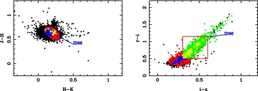
The selected sample in the (J − H, H − K) and (r − i, i − z) diagrams. See the text for details. Black circles mean selection via Te, log g and radius; red circles: subsample via JHK photometry; green circles: subsample via JHK plus riz photometry; yellow stars: SC L1 subsample; blue squares: SC L2 subsample. The red area in right panel corresponds to the region r − iKIC = 0.50–1.15, i − zKIC = 0.30–60. The eclipsing binary ID86 is marked in blue.
Fig. 2 compares our selected sample with the M dwarfs in the DCh13 catalogue. As mentioned before, only 43 stars in the DCh13 list were observed in SC mode, and 37 of them are found in our lists (34 in L1 and three in L2). Six objects still remain, which are neither included in the L1 nor in the L2 list. They constitute the subsample L3 and are listed at the end of Table 1. The reasons why they were not found in L1 or L2 are well justified: ID93 has no KIC values available for i − z or Te (moreover, its J − H and H − K indices seem wrong; as shown in Fig. 2); the KIC listed radii for ID90 and ID95 are too large (>1.0 R⊙); ID92 and ID94 have MDE <20 pixel and, finally, ID91 has H − K = 0.100 mag, just below our selected limit of H − K > 0.100 mag. On the other hand, there are 22 objects in Table 1 which are also in Baran et al. (2011b), 15 belong to L2 and seven to L1. Furthermore, there is only one object (ID31) common to Baran et al. (2011b) and DCh13, and another one (ID10) common to Rodríguez-López et al. (2015a) and DCh13.
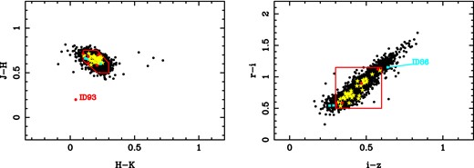
The DCh13 sample in the (J − H, H − K) and (r − i, i − z) diagrams. Black circles mean stars in the DCh13 catalogue; yellow stars: objects in the DCh13 catalogue common to our L1 list; blue squares: objects in the DCh13 catalogue common to our L2 list; red circles: objects in the DCh13 catalogue but not in our L1 or L2 lists. The red areas show the regions for the subsamples via JHK (left) and riz (right) photometry. The locations of ID93 and ID86 are also indicated in the figures.
Our sample of 95 objects listed in Table 1 is very similar to what would be obtained if we considered the more recent catalogue of stellar properties for Kepler targets by Huber et al. (2014), assuming the same initial ranges for Te, log g and radius adopted above. In fact, all the targets included in our L1 list, or common to the DCh13 catalogue, would be included in the new resulting sample. The most remarkably difference concerns the target ID79 which seems not to be a M dwarf star: Huber et al. (2014) adopt Te = 4583 K and log g = 2.334 from Molenda-Zakowicz et al. (2013), who derived a G9III spectral type, while Baran et al. (2011b) obtained K2III. Nevertheless, we keep this target in our list for completeness.
3 DATA ANALYSIS
The Kepler mission (Borucki et al. 2010; Gilliland et al. 2010; Jenkins et al. 2010; Koch et al. 2010) provides photometric time series in two types of cadences: LC and SC data sets. Each individual measurement is composed of a 6.02 s exposure with 0.52 s readout time. Each data point in LC mode is the integration of 270 exposures to give a data point every 29.43 min, whereas the SC data consist of nine exposures giving one data point every 58.85 s. Both cadences are stored on-board and downlinked to Earth roughly every month. The measurements in LC mode are stored for all stars in the mission (∼156 000 selected stars up to 16th mag covering a field of view of 115 deg2), but downlink limitations restrict SC mode targets to only 512 each month, which are selected depending on the priorities at each time. The upper frequency limit, given by Nyquist frequency, in searching for pulsations in the Kepler time series, is fNyq = 24.5 cd−1 for LC and fNyq = 734.1 cd−1 for SC mode. Hence, we are only interested in the SC data sets in order to investigate the possible detections of M dwarf pulsations predicted by Rodríguez-López et al. (2012, 2014). In particular, those in the ∼20–40 min range (f ∼ 35–75 cd−1) for old low-mass models or in the range of the solar-like oscillations. The Kepler light curves are available in the Mikulski Archive for Space Telescope (MAST1). We downloaded all the SC mode datafiles available for Q1 to Q16 quarters. Column 6 of Table 1 lists the number of months available for each star of our sample.
The Kepler time series are available in two forms: (a) the SAP (Simple Aperture Photometry) or ‘raw’ curves which are nearly the original fluxes where only basic calibrations have been applied, and (b) the PDC (Pre-Search Data Conditioned) or ‘corrected’ curves where some algorithms have been applied in order to remove instrumental perturbations –as drifts, jumps and outliers – from the original light curves. The PDC data sets were mainly aimed to facilitate the search of planetary transits and they are in constant evolution with new and more refined procedures being established regularly. Nevertheless, some caution is needed when detailed frequency analyses of the light curves are performed, because some stellar variability may have been modified by the algorithms used. Hence, we preferred to use the SAP curves and to apply our own procedure to correct them, although sometimes the PDC curves will also be used for checking purposes.
First, within each monthly (quarter Qi.j) time series, the SAP flux in e−/s was converted to magnitudes, the zero-point of the data set was shifted to median = 0.0 and a 1° polynomial was fitted to remove linear trends. Moreover, the overall shape of the light curve was derived by fitting a spline curve to means, in 4 h intervals, of the data. This works well in most cases, but when short-period high-amplitude variations take place, the binning intervals need to be smaller. Using the smoothed curve, the outliers are removed by an iterative procedure. In the present work, we apply a relaxed 4-σ clipped factor for deviations from the residual light curve. With this procedure, large enough flares and eclipses produced by planetary transits are also removed from the light curves. Finally, the median value of each data set is again shifted to a new value of median = 0.0. Secondly, because we are interested in looking for short-period periodicities as those predicted by pulsations in M dwarf stars, the long-term variations present in the light curves due to stellar activity or binarity are removed. To do this, the light curves within each quarter Qi.j are binned each 4 h, in order to build smoothed mean light curves by cubic spline interpolations to detrend the original light curves.
Fig. 3 presents two examples of stars analysed with this procedure. The SC time series for ID24 and ID55 were collected at quarters Q3.2 and Q2.1, respectively. In both cases, their variability seems to be produced by rotational modulation with periodicities of 8 d and 10 d, with a large number of flares showing in the light curves of ID55. After the long-term variability is removed from the light curves, the periodograms remain mostly flat. No pulsations are detected in the amplitude spectra. Some power still remains in the low-frequency region for ID55 because of the residuals produced by the flares (main peak at f = 4.5 cd−1), but this does not affect our results. In the case of ID24, one significant peak, denoted as a(31), is shown in the periodogram which corresponds to the well-known and catalogued Kepler artefact in the 31–32 cd−1 region (see table 5 of Christiansen et al. 2013 – Kepler Data Characteristics Handbook – or fig. 8 of Baran 2013). For ID55 another artefact, a(20 −), is shown at ∼18 cd−1, which was also catalogued by Baran (2013) for the Q2.1 quarter.
![Examples of analysed light curves: ID24 (left panels, rotational modulation with periodicity of 8 d, Q3.2, K7V) and ID55 (right panels, rotational modulation and flares, P = 10 d, Q2.1, M0V). Top panels: original SAP light curves after correction for long-term linear drifts and outliers (including flares for ID55). Middle panels: residual light curves after long-term variations are removed. Bottom panels: resulting periodograms in the [0,100] cd−1 region. The significance levels at S/N = 4.0 are shown. Artefacts, a(31) at 31.4 cd−1 for ID24 and a(20 −) at ∼18 cd−1 for ID55, are present. Some power still remains for ID55 at low frequencies due to residuals from flares.](https://oup.silverchair-cdn.com/oup/backfile/Content_public/Journal/mnras/457/2/10.1093/mnras/stw033/2/m_stw033fig3.jpeg?Expires=1750791358&Signature=V6u~PvGorZhNY21jrWBvgBLeOAiL7uUwaiOnfaO5DZv5to-r-AQEvUkF68G1vM0kXhGAE3hvr-szl4-rTxbgrWBntRiBUtEPCm1KBEtaWezDEIBZCdJl0HMDB56KG9~LA8NwS4MsgSeW6a6oIMZwDgTFINc9dGbsVYhgKAvwR8qVWtoVpZYWEfCzIaA6pD1ZnnblpOD1bO3FYwUe-HUmVcU-3KrtqdzA77JYd-MinMUPIcf6FsLaDm4O4OB2Ui~lDMM0a0rPXFHBUZJw6N1WLyb1-1RMO4pcDoZjmfZpQEunaslJKzkXhqLzcd3QK~KdaIUkwi6U0e8SUdIh2dF5jw__&Key-Pair-Id=APKAIE5G5CRDK6RD3PGA)
Examples of analysed light curves: ID24 (left panels, rotational modulation with periodicity of 8 d, Q3.2, K7V) and ID55 (right panels, rotational modulation and flares, P = 10 d, Q2.1, M0V). Top panels: original SAP light curves after correction for long-term linear drifts and outliers (including flares for ID55). Middle panels: residual light curves after long-term variations are removed. Bottom panels: resulting periodograms in the [0,100] cd−1 region. The significance levels at S/N = 4.0 are shown. Artefacts, a(31) at 31.4 cd−1 for ID24 and a(20 −) at ∼18 cd−1 for ID55, are present. Some power still remains for ID55 at low frequencies due to residuals from flares.
The computer program package Period04 (Lenz & Breger 2005) was used to perform the frequency analyses of each target in the region up to 100 cd−1. Following some authors (Breger et al. 1993; Kuschnig et al. 1997), one peak can be considered significant when its amplitude signal-to-noise ratio (S/N) is larger than 4.0. When various months are available for the same target, the quarters are merged together and the full time series is analysed. No zero-point corrections are necessary in the merging because the fluxes were previously zero-centred at each quarter. Nevertheless, if we are interested in the analysis of the ‘original’ light curves, just before extracting the long-term variations, sometimes it is necessary to match the end of one quarter to the start of the following one. This is done in an automatic and standard mode whenever possible, and manually corrected for the more complicated cases.
4 RESULTS
4.1 Light curves
A visual inspection of the original SAP light curves and period estimates was carried out using Period04 (Lenz & Breger 2005). The results of this analysis are summarized in Columns 7 and 8 of Table 1 where a variability type and estimation for the main periodicity is assigned to each star. Almost all the objects present some type of variability commonly associated with stellar activity, as expected for late and low-mass stars. Many of them show regular periodicities as clear examples of rotational modulation (ROT) produced by rather stable spots corotating with the star (see Fig. 3). We used the term ‘Irr’ to denote irregular light curves with probably multi- or quasi-periodicity. Some light curves show what it seems long-period variability with an undetermined period of variation within the lengths of our available time series, and the term LPV(?) is used for them. In a few cases, no confident variability is detected either in the light curves or in the periodograms, and they are classified as probable constant stars, with the term const(?). Many stars present flares (F); most of them are found to be ROT+F. The term ECL is used for eclipsing binaries and T for stars showing typical features of transits in their light curves (eclipses) or in the periodograms (regularly spaced sharp peaks).
A number of stars in Table 1 have available spectral types in the bibliography, mostly determined by Baran et al. (2011b). A few stars seem not to be dwarfs according to their tabulated spectral classes: one object in the L1 list: ID4(K2II) and seven in L2: ID46(K4III), ID50(K1.5III), ID51(K4III), ID54(K2III), ID60(K4III), ID79(K2III) and the eclipsing binary ID89(M1III). All, except the later, present irregular light curves and small amplitudes which resemble those stars classified as ACT (stellar activity) in Debosscher et al. (2011). Similar light curves are also shown by ID45, for which no spectral classification is given. However, their variability is due to solar-like oscillations in red giants (two examples are shown in the top panels of Fig. 4; see also e.g. Bedding et al. 2010; Balona et al. 2013; Huber et al. 2014). This is confirmed when the corresponding LC time series (quarters Q1 to Q16) are analysed and amplitude excesses, as Gaussian-like envelopes of regular peaks, appear in well-defined regions of the periodograms as shown in the bottom panels of Fig. 4. The same analysis has been performed for the rest of stars in Table 1, but with unsuccessful results. We list in Table 2 the seismic parameters resulting from our analysis: νmax (frequency of maximum amplitude of the envelope of peaks), Amax (maximum amplitude) and Δν (the so-called large separation between consecutive radial orders of the same spherical angular degree, l). We derived νmax and Amax assuming a Gaussian-shaped envelope of peaks in a window of about [−νmax,+νmax] and Δν as twice the mean frequency separation between regular and consecutive peaks within the same window. Their error bars are listed in Table 2 as the σ of the corresponding mean values. The last column lists the theoretically predicted values ΔνH using the empirical relation Δν = |$\alpha \nu _{\rm max}^{\beta }$|, with α = 0.263 and β = 0.763 (Hekker et al. 2010; Huber et al. 2011). A very good agreement is found between the observed and predicted values.
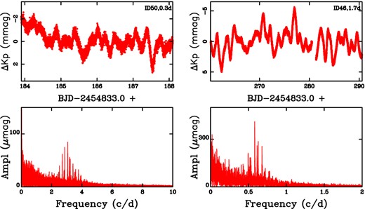
Examples of red-giant stars in our sample showing solar-like oscillations. Top panels: light curves obtained from one month of available measurements in SC mode. Bottom panels: resulting periodograms for quarters Q1–Q16 in LC mode.
| ID | ST | νmax | Amax | Δν | ΔνH |
|---|---|---|---|---|---|
| (μHz) | (μmag) | (μHz) | (μHz) | ||
| 4 | K2II | 3.8(6) | 450(10) | 0.84(18) | 0.73 |
| 45 | 5.8(6) | 340(10) | 1.02(14) | 1.01 | |
| 46 | K4III | 6.8(6) | 410(10) | 1.16(12) | 1.14 |
| 50 | K1.5III | 35.9(6) | 85(5) | 4.16(24) | 4.04 |
| 51 | K4III | 5.8(6) | 350(10) | 1.06(20) | 1.01 |
| 54 | K2III | 27.1(6) | 60(5) | 3.04(26) | 3.26 |
| 60 | K4III | 8.1(6) | 500(10) | 1.39(23) | 1.30 |
| 79 | K2III | 7.6(6) | 180(10) | 1.20(12) | 1.24 |
As mentioned in Section 2, contrary to its original KIC values, the revised stellar parameters of ID79 listed in the catalogue for Kepler targets by Huber et al. (2014) indicate that this object is a giant star. However, all the other seven targets in Table 2 are misclassified as dwarfs, as suggested by the stellar parameters (Te, log g and radius) listed. These eight red-giant targets are excluded of our frequency analyses in the next sections.
There are also eight targets in our sample which happen to be eclipsing binary systems. In all cases they show flares, meaning that at least one of the components is an active star. Some of them present short periods (three under 8 h) and deep eclipses that make very difficult the investigation for detecting pulsations in the periodograms at the level of μmag. Even if binarity is extracted from the light curves and the temporal scale of the binnings is reduced to only 2 h, the remaining residuals are too large to derive any confident diagnostic on pulsations at the level of reliability obtained for the rest of the targets. This is so because the noise levels in the periodograms are largely increased by leakage effects.
The majority of the stars in Table 1 present transits and were classified as KOI targets in the Kepler planet candidates’ list by Batalha et al. (2013). Many of them were later confirmed as exoplanets,2 whereas other still remain as just candidates. This is expected from our sample, because Kepler SC observations of M dwarfs were commonly devoted to objects of interest in looking for exoplanets. Many of them have also been detected in our analysis as it is shown in column 7 of Table 1. When the eclipse depths are large enough they are found directly via visual inspection of the light curves, and almost all were detected via Fourier analysis (see some of the panels in Figs 5 and 6). This method is powerful, in particular for short orbital periods, as it has been already shown by earlier authors [see e.g. Charpinet et al. (2011), Sanchis-Ojeda et al. (2013, 2014) and Silvotti et al. (2014).
![Periodograms in the [0,100] cd−1 region for stars common to DCh13 (continues in Fig. 6). Some spurious frequencies are marked; the most common are artefacts at ∼ 31–32 cd−1. The symbols mean: a: artefact; F: flares; T: transits; ECL: eclipsing. The S/N = 4.0 significance levels are shown as solid blue (in the electronic version) horizontal lines.](https://oup.silverchair-cdn.com/oup/backfile/Content_public/Journal/mnras/457/2/10.1093/mnras/stw033/2/m_stw033fig5.jpeg?Expires=1750791358&Signature=P9JviFb-6EbNUlfVk1vMAsvfoZIZD0Wi0tIP8DSXeb43ZHZ7SbTFreGypV90ZtucSj6pb9qi-kLyidS0-cwPpxASlPGo0U68fCLrwGt00sQOQYq8Xs5j8LSCnhqAIKexbDiCM3muDoP20yPDmgzK4~nOvJd2-ZLs6Q6AWHglMRHDhRnVcycdaFuVpi6C3jtx93A0vQEUH~AvBxrRQYoIM8e7QCvGGpMpbNWxcFohw-Hd22OMIjpyHyrApIckxC4BTIUYr6oVIWzrLgmWOtmsUvau9VM7D~IuzJNbZnJQmEzh7UK28EgLQ-L4t7rjs-cGdf~yel25JPARjSdqs84Hfg__&Key-Pair-Id=APKAIE5G5CRDK6RD3PGA)
Periodograms in the [0,100] cd−1 region for stars common to DCh13 (continues in Fig. 6). Some spurious frequencies are marked; the most common are artefacts at ∼ 31–32 cd−1. The symbols mean: a: artefact; F: flares; T: transits; ECL: eclipsing. The S/N = 4.0 significance levels are shown as solid blue (in the electronic version) horizontal lines.
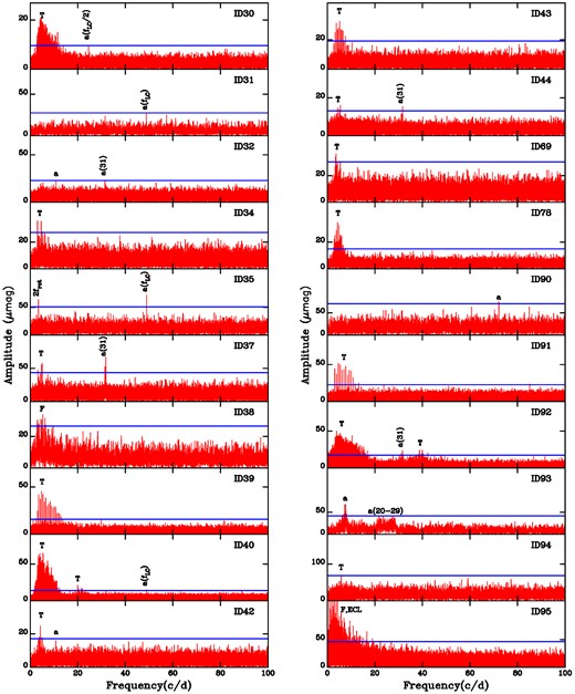
Continuation of Fig. 5.
4.2 Frequency analysis in region <100 cd−1
We present the results of our frequency analysis in Figs 5 and 6 for the [0,100] cd−1 frequency range for stars common to the DCh13 catalogue (with the exception of the short-period eclipsing binary ID86), the results for the rest of the stars in the sample being very similar. Column 9 in Table 1 lists the detection thresholds obtained for each star, in the [20,100] cd−1 frequency range, determined as four times the mean noise level over that range (blue solid lines in Figs 5 and 6). The detection limits in the [100,735] cd−1 range have also been determined and listed in Column 10. For practically all cases, the significance levels in the higher frequency region are very similar to those in the [20,100] cd−1 region. This means that the noise levels determined in the [20,100] cd−1 region are close to the true white noise levels and the resulting T[20,100] values are a good measure for the significance levels in that region. We also find very good agreement with the detection thresholds determined for the same stars by Baran et al. (2011b) and Rodríguez-López et al. (2015a).
We do not find any significant peak that can reliably be attributable to pulsations in the region of interest for old low-mass models, roughly ∼35–75 cd−1. Nearly all the periodograms are shown to be flat for f ≳ 20 cd−1 and, many of them for f ≳ 10 cd−1. Nevertheless, many panels show that some power remains in the low-frequency domain, which is caused by flares, transits or their residuals, as indicated by the F and T symbols. The larger the number of flares or transits, the larger the residual power. Despite many of them being cleaned from the light curves, there are many others that can not be removed because of their very small amplitudes or our relaxed 4σ criterion for outliers. Moreover, even when they are well removed, the introduced gaps also produce power in the low-frequency regions. When the power is mainly produced by binary eclipses, additional leakage effects may propagate over the low-frequency domain.
Periodograms in Figs 5 and 6 show a number of significant peaks which, in all cases, are matched to spurious frequencies already catalogued in table 5 of the Kepler Data Characteristics Handbook by Christiansen et al. (2013) and/or in Baran (2013). The most frequent peak in the sample is the well-known artefact a(31) which takes place at 31–32 cd−1 region for different quarters. Moreover, the artefact related to the LC readout time, fLC = 48.94 cd−1 and its first harmonic, 2★fLC (ID11), or its subharmonic, fLC/2 (ID30), are also present. The star ID93 clearly shows the artefact a(7.5) related with the reaction wheels housing temperature (Christiansen et al. 2013) and another one in the 20–29 cd−1 region also detected by Baran (2013) for data sets in quarter Q1, the same available for ID93. The significant peak in ID27 at a(11.8) is also identified by Baran (2013) for Q14 and probably it is also related with the nearly significant peaks at ∼10.8 cd−1 in both ID32 and ID42. ID1 presents two peaks at 15.2 cd−1 (S/N = 4.4) and 16.5 cd−1 (S/N = 4.3), which are probably related with the ‘20 −’ artefacts found in the same region by Baran (2013) for various quarters. The same is also valid for the significant peaks at 18.2 cd−1 (S/N = 4.6) (20−) and 22.8 cd−1 (S/N = 4.2) (20 +) shown in the periodogram of ID12. Concerning ID35, an isolated peak at 3.395 cd−1 corresponds to the first harmonic of its stellar rotation period (frot = 1.698 cd−1) in very good agreement with the value derived by Rappaport et al. (2014). The significant peak (72.1 cd−1, S/N = 4.3) in ID90 is located just in the region where the artefacts U1a = 71.4 cd−1 and U1b = 73.6 cd−1 (Baran 2013) take place. Power at ∼40 cd−1 in ID92 is due to transits, as it is in the low-frequency region. Transits are probably also the cause for the weak power shown by ID94 in the low-frequency region, where five planets were confirmed. ID29 also presents two weak peaks at 29.1 cd−1 (S/N = 3.9), close to the artefact U2 = 29.4 in table 5 of Christiansen et al. (2013), and 96.7 cd−1 (S/N = 4.1), which might be related with 2*fLC.
Additional slightly significant peaks in the periodograms, which have not been identified as catalogued artefacts, are shown for some stars as ID40 (f = 89.0 cd−1, S/N = 3.8) or ID91 (f = 23.7, S/N = 4.0; F = 85.1, S/N = 4.0). However, these peaks change in amplitude or even vanish from the periodograms when different subsamples of the full time series are investigated. They seem to be spurious peaks, not attributable to pulsations.
4.3 Frequency analysis in region >100 cd−1
The frequency analysis was also performed for frequencies >100 cd−1 in order to search for possible solar-like oscillations, as predicted by the models in Rodríguez-López et al. (2014). The analysis was carried out in the [100,735] cd−1 range, because of the Nyquist limit for the Kepler SC time series. The computer program SigSpec (Reegen 2007) was used in automatic mode for the full sample. For each time series, SigSpec works iteratively looking for significant peaks in the periodograms until the default limit for the spectral significance (sig) parameter, sig = 5.0, is reached. A SigSpec limit value of sig = 5.46 is approximately equivalent to S/N = 4.0 using Period04 for the same time series (Reegen 2007; Kallinger et al. 2008). When the periodograms are dense (i.e. the number of significant peaks is very high), we must be cautious and much more conservative concerning the limit used for the sig parameter (see e.g. García-Hernández et al. 2009, 2013; Chapellier et al. 2011), but this was not the case here, as we will see below.
After all the significant peaks are pre-whitened, the noise levels and S/N values of each peak are determined. The majority and most powerful significant detected peaks are identified as artefacts related with fLC. They are frequently shown as various consecutive harmonics of fLC, up to the 15th, with the seventh, eight and nine terms commonly being the strongest ones. Some examples are shown in Fig. 7. Most of the remaining significant peaks have also been already identified as the U sequence of artefacts in Baran (2013) and/or Christiansen et al. (2013) (see also Fig. 7).
![Periodograms in the [100,735] cd−1 region for stars in Table 1. Some spurious frequencies clearly stick out in the periodograms. ‘n’ means artefact caused by harmonics of fLC. The S/N = 4.0 (solid) and S/N = 3.0 (dashed) significance lines are also shown.](https://oup.silverchair-cdn.com/oup/backfile/Content_public/Journal/mnras/457/2/10.1093/mnras/stw033/2/m_stw033fig7.jpeg?Expires=1750791358&Signature=LXrxzVt6SuyDXHmUzKsJVyL0pr8uosrdpojSXWMzOsaUyWBC8oY56AACG1Mxgq8CfgGl1vgEwlzoEEIi4sCU7tX0-A7pe3s58dE1-DTT2cbZ~h134y9vqZGPKGgyIIMzxActwyq2wvyPI4L1uwbnJX8B6eLKF4CmsukGw40UuxOU-A4ZIH8r6mBFLKCcIhlYWclHTFZHamqqJ5CoK~hW8hPqpQXF3t6niGO5kJi56H7aSPJhQC8Icad-MUwyRPaseQgg4mMwzyoEib4GhVcG0gdi52MoAiPF1kLOmCfuzyUC4YPz8IyhI3dZuoSsXEpmclCQZDoFc0KmV0boLo3MTw__&Key-Pair-Id=APKAIE5G5CRDK6RD3PGA)
Periodograms in the [100,735] cd−1 region for stars in Table 1. Some spurious frequencies clearly stick out in the periodograms. ‘n’ means artefact caused by harmonics of fLC. The S/N = 4.0 (solid) and S/N = 3.0 (dashed) significance lines are also shown.
There are only a few remaining significant peaks in the periodograms, which are not catalogued as artefacts in the bibliography. They are listed in Table 3, showing that there is not any preference for frequency distribution and that all have little significance. Nearly all have sig<6.0 and S/N<4.5, mean values of <sig> = 5.5(±0.4) and <S/N> = 4.3(±0.2), very close to the limit of significance commonly accepted for this kind of analysis. Furthermore, Table 3 also lists a few pairs of closed peaks obtained for different stars in similar quarters: (ID32, ID53), (ID9, ID40), (ID64, ID83). They might be related to each other and be, in fact, artefacts, or simply spurious peaks. In order to test our results, the corresponding PDC available light curves (PDC-quickMAP version; Christiansen et al. 2013; Thompson et al. 2013) were also analysed using the same procedure as for the SAP curves. The results obtained are identical to those shown above.
Significant peaks (Sig≥5.0) in the [100,735] cd−1 region which are not catalogued as artefacts in the bibliography. The terms ‘single files’ and ‘multiple files’ refer to time series with only one, or more than one, month of observations in SC mode, respectively.
| ID | Freq | Ampl | Sig | S/N | ID | Freq | Ampl | Sig | S/N | ID | Freq | Ampl | Sig | S/N |
|---|---|---|---|---|---|---|---|---|---|---|---|---|---|---|
| (cd−1) | (μmag) | (cd−1) | (μmag) | (cd−1) | (μmag) | |||||||||
| Single files | 20 | 653.529 | 13.5 | 5.6 | 4.1 | 70 | 697.620 | 29.2 | 5.5 | 4.3 | ||||
| 2 | 416.593 | 54.9 | 5.6 | 4.4 | 25 | 122.895 | 13.8 | 5.2 | 4.1 | 238.014 | 28.7 | 5.3 | 4.2 | |
| 201.319 | 52.3 | 5.1 | 4.2 | 32 | 307.476 | 23.8 | 5.7 | 4.2 | 581.865 | 28.4 | 5.2 | 4.2 | ||
| 41 | 516.611 | 7.1 | 6.8 | 4.7 | 34 | 419.145 | 31.4 | 5.9 | 4.6 | 73 | 163.316 | 91.9 | 5.0 | 4.4 |
| 52 | 546.021 | 9.9 | 5.4 | 4.1 | 593.525 | 30.5 | 5.6 | 4.5 | 80 | 731.935 | 50.7 | 5.4 | 4.2 | |
| 82 | 596.562 | 13.0 | 5.4 | 4.1 | 35 | 622.890 | 50.5 | 5.3 | 4.0 | 239.156 | 49.4 | 5.2 | 4.0 | |
| Multiple files | 339.019 | 49.5 | 5.1 | 4.0 | 81 | 486.609 | 19.6 | 5.6 | 4.2 | |||||
| 1 | 564.352 | 75.0 | 5.2 | 4.2 | 37 | 476.535 | 46.0 | 5.2 | 4.3 | 83 | 351.890 | 25.7 | 5.6 | 4.3 |
| 9 | 312.040 | 36.9 | 5.4 | 4.1 | 40 | 313.780 | 16.1 | 6.1 | 4.7 | 707.705 | 25.0 | 5.3 | 4.2 | |
| 442.185 | 38.6 | 5.4 | 4.3 | 726.095 | 15.1 | 5.3 | 4.4 | 84 | 589.594 | 28.8 | 5.9 | 4.2 | ||
| 10 | 658.334 | 18.1 | 5.1 | 4.1 | 42 | 422.490 | 20.3 | 6.9 | 4.7 | 87 | 280.359 | 40.4 | 5.5 | 4.3 |
| 708.672 | 18.0 | 5.1 | 4.1 | 53 | 308.355 | 44.9 | 5.0 | 4.0 | 92 | 131.984 | 17.3 | 5.7 | 4.2 | |
| 14 | 166.730 | 14.9 | 5.1 | 3.9 | 64 | 192.904 | 21.9 | 5.5 | 4.1 | 602.925 | 16.2 | 5.1 | 4.0 | |
| 15 | 273.235 | 29.9 | 5.5 | 4.3 | 706.080 | 20.1 | 5.0 | 3.8 | 94 | 205.799 | 76.0 | 6.0 | 4.5 |
The analysis carried out in the [100,735] cd−1 region means that we have investigated oscillations as short as ∼2 min. If we consider the well-known scaling relation for νmax from Kjeldsen & Bedding (1995, equation 10) together with the model predictions by Rodríguez-López et al. (2014), solar-like pulsations in M dwarfs can reach frequencies ∼1000–1400 cd−1, far beyond the Nyquist limit, given by fNyq = 734.1 cd−1. Nevertheless, our frequency analysis is also valid to test the existence of possible periodicities in this frequency domain, because of the Nyquist aliases, which must show up in the region below fNyq, if real peaks occur in the super-Nyquist regime (see e.g. Reed et al. 2012; Murphy, Shibahashi & Kurtz 2013). In order to confirm this assumption, we have performed some simulation tests: we have considered the SC time series of ID90 and different synthetic signals (periodicities) have been simultaneously added at different frequencies (from 835 cd−1 to 1400 cd−1). The results show that these peaks also show up in the region below fNyq as Nyquist aliases, with practically the same amplitudes as the real ones. We find no peak that can be attributable to solar-like oscillations, as their typical amplitude excess, with regular peaks forming a roughly Gaussian-shaped envelope, is not found in the periodograms. Hence, we conclude that no solar-oscillations are detected in our analysis.
In order to further investigate these results, the corresponding power spectra of each target were considered, smoothed over 1 μHz and plotted on log–log scales (Chaplin et al. 2010, 2011; Hekker et al. 2010), but with unsuccessful results. From visual inspection of the power spectra, neither power excess nor regular structures which could be attributable to solar-like oscillations are found. However, we estimate that we can now reduce our detection limits to roughly the top of the grass level in the amplitude spectra, which approximately correspond to the S/N = 3.0 significance levels as shown in the panels of Fig. 7.
Periods at maximum power (Pνmax, in minutes) and bolometric amplitudes (Abol, in μmag) predicted for solar-like oscillations in M dwarfs using the excited models from Rodríguez-López et al. (2014) and scaling relations for amplitudes of solar-like oscillations from Corsaro et al. (2013), models M4, β and M2. See text for details.
| Cases | Mass | P | Excit. | Comments | e-fold | Pνmax | Abol(M4, β) | Abol(M2) |
|---|---|---|---|---|---|---|---|---|
| (M⊙) | mechan. | <age | (min) | (μmag) | (μmag) | |||
| A | 0.10–0.40 | 4–11 h | ϵ (D) | Age ≤ 2 Myr | X | 30 min–1 h | 90–130 | 16–30 |
| B1 | 0.40–0.60 | 1–2 h | F-b | Age ≤ 50 Myr | X | 2–4 | 5–7 | 2–3 |
| B2 | 1–3 h | F-b, ϵ (He3) | g modes | 2–3 | 4–5 | 2–3 | ||
| C | 0.20–0.30 | 20–30 min | ϵ (He3) | 1–3 | 4–6 | 1–3 | ||
| D | 0.35–0.60 | 20–60 min | F-b | 1–3 | 4–6 | 1–3 |
The results are presented in Table 4. For the sake of simplicity, we include only the maximum and minimum values obtained for the period at maximum power (Pνmax) and the bolometric amplitude (Abol), as Columns 7 and 8 of Table 4. The values for the expected amplitudes are very small compared with the detection thresholds determined for our targets. Only in a few cases, our targets present threshold values below 10 μmag for an S/N = 4.0 significance limit.
We would like to point out that the empirical scaling relations used have not been calibrated for M dwarfs, and that only by discovering M dwarf solar-like pulsations will be possible to fine-tune them. However, we note that Pνmax agree well with those determined by RL14 (Table 3), using a different method proposed by Mullan (2010) for the selection mechanism of solar modes, although the range of periods is larger here, as we calculate them also for M dwarf models with subsolar metallicities and different values of the mixing length parameter. That said, we found that the highest oscillation amplitudes (∼100 μmag) correspond to very young models (ages less than 2 Myr) still in the contracting phase. From the oscillation analysis in RL14, the e-folding time, i.e. the time that the oscillation needs to increase its initial unknown amplitude by a factor e, is longer than the age of the model (this is also true for case B1). This means that unless the initial amplitude is large, the modes are not likely to be excited. The fact that we do not detect oscillations in this period range, even if the detection limits of our sample are far below 100 μmag, could be explained by this, or more likely, because none of these very young objects is found in our sample.
For cases B1, B2, C and D, Pνmax are in the 1–4 min range; as said before, the shortest 1 min periods could still be detected by Kepler SC as aliases peaks reflected from super-Nyquist regime; however, the expected low amplitudes, of ∼5 μmag, could not be detected within our sample. Moreover, more pessimistic amplitude predictions (∼1–3 μmag) are obtained if a simpler model such as M2 in C13 is used, as shown in the last column of Table 4.
5 DISCUSSION AND CONCLUSIONS
We have carried out a survey to search stellar pulsations in M dwarf stars in the Kepler SC data base. This investigation covers all the objects observed in SC mode, which are also present in the cool and dwarf stars’ list of DCh13. In order to extend the sample as much as possible we have expanded the selection via stellar parameters (temperature, surface gravity and radius) with available KIC values, JHK and riz photometry, giving a total of 95 objects.
Almost all the stars in the sample show some type of variability, commonly associated with stellar activity, and only very few stars seem to be constant. Even in some of these cases, the objects are found to be host of planetary systems. Many stars show flares, which are usually associated as clear evidence for rotational modulation, and are assigned the ROT+F class. It is expected that many of the remaining targets would also show flares in longer time-scales if their corresponding LC data series were investigated, despite the much poorer sampling. The sample also includes eight eclipsing binaries, three of them with very short orbital periods (<8 h) and deep eclipses. The majority of the targets in our sample present transits, most of which have been detected in our frequency analysis due to the typical features, as regularly spaced sharp peaks, shown in the periodograms. Moreover, eight objects have been reported as red-giant stars showing solar-like oscillations. We confirm this classification by analysis of their LC time series, and as a result, these stars were excluded from our sample. Seven of them are misclassified as dwarfs in the Kepler stellar properties catalogue of Huber et al. (2014).
In total, 87 objects were analysed as M dwarf candidates for detections of stellar pulsations. Most of them were observed during several months, which reduces the noise levels and, consequently, the thresholds for detection of significant pulsational peaks in the periodograms. We used Fourier analysis in the versions of Period04 (Lenz & Breger 2005) and SigSpec (Reegen 2007) to search for periodicities. Almost all the significant peaks (S/N≥4.0) found in the periodograms were already well-identified as artefacts in Christiansen et al. (2013) and/or Baran (2013). The most frequent spurious peak detected in the <100 cd−1 region is the well-known artefact a(31), which takes place in the 31–32 cd−1 range, together with that related to the long-cadence readout time, fLC = 48.94 cd−1. The majority and most powerful significant peaks detected in the >100 cd−1 region are partial series of consecutive harmonics of fLC, up to the 15th, with the seventh, eighth and ninth terms frequently as the strongest ones, as it was expected from earlier investigations.
However, we have not detected any significant signal that can reliably be attributable to pulsations in the [ ≳ 10,100] cd−1 frequency domain. Our detection limit is below 10 μmag for the brightest objects, 20 μmag for about 40 per cent of the objects and 50 μmag for nearly all (80 per cent) the objects in the sample. We have also investigated the periodograms in the >100 cd−1 region searching for possible solar-like oscillations, but we conclude that none is detected with periodicities longer than ∼1 min ( ≲ 1400 cd−1). The corresponding power spectra have been also investigated, but with unsuccessful results too.
The fact that we do not detect solar-like stochastic oscillations, excited by turbulent convection, may be due to the predicted amplitudes (∼2–5 μmag) falling below our typical detection thresholds. However, we have to keep in mind that the scaling relations used are not calibrated for M dwarfs and some room for discrepancies in the predicted values is possible. We can also speculate that selection mechanisms are at work that prevent all M dwarfs to be stochastic pulsators, so only a small fraction could pulsate.
Regarding pulsations excited by classical thermodynamic methods, ϵ or flux-blocking mechanisms, as proposed by Rodríguez-López et al. (2012, 2014), the fact that we have not detected evidence in any star in our sample could be due to several facts.
The excited coherent oscillations may be of very low amplitude and not photometrically detectable to the current threshold limits of this sample. In the case of classical excitation mechanisms, we do not really know what to expect about the oscillation amplitudes, as the oscillation codes used in the analysis are unable to predict them, and the range of observed amplitudes for other classical pulsators is large. For instance, in the case of Gamma Doradus pulsators, also excited by the flux-blocking mechanism, the observed amplitudes cover a range from a few μmag to some hundredths of a magnitude.
The sample is not statistically significant: we are confident that at least 52 stars can be regarded as M dwarfs. Of them, 43 had been already catalogued in the DCh13 M dwarfs’ list and nine more already analysed by Baran et al. (2011b) and Rodríguez-López et al. (2015a) (six of them have also been included in the present work.). Furthermore, on the basis of ground-based observations, 120 M dwarfs were analysed at a typical detection limit of ∼1 mmag, with unsuccessful results too (Baran et al. 2011a, 2013; Krzesiński et al. 2012). This would mean that the possible pulsational amplitudes should be very small, below a few μmag, or that the rate of pulsating–non-pulsating M dwarfs is very low. We will still pursue a photometric detection of pulsations from the work-in-progress analysis of the most precise M dwarfs SC data available supplied by the Kepler K2 mission3 (Rodríguez-López et al. 2015b).
Oscillations are not photometrically detectable due to cancellation effects: photometry is more sensitive to intensity variations caused by the pulsations rather than velocity variations. On the contrary, spectroscopy is more sensitive to velocity variations, with a smaller contribution of the intensity variations. Townsend (1997) theoretically shows that, for certain values of the frequency, photometric variability may be practically absent, while still spectroscopic variability could be detected. Other pieces of evidence, such as granulation noise being higher in photometry than in spectroscopy (Fröhlich et al. 1995; Gabriel et al. 1995) and that a 10 μmag photometric amplitude would result in 0.7 m/s Doppler shift (Zima et al. 2006), gives us confidence to believe that the discovery of observational M dwarfs pulsations will come hand-in-hand through time series spectroscopy of high temporal and spectroscopic resolution. This is the aim of the Cool Tiny Beats Project (Berdiñas et al. 2015) using HARPS (Mayor et al. 2003) and HARPS-N (Cosentino et al. 2014), the most precise optical spectrographs to date. This spectroscopic search will also be extended soon to CARMENES spectrograph (Amado 2015), as one of its additional science cases, whose first light is expected at the end of 2015.
We also have to consider the possibility that M dwarfs do not pulsate, that the damping regions within the star exceed the excitation of the driving ones, and the amplitude reaching the surface is so tiny as not to be detectable. Limitations in the implementation of physical processes in the structural models and/or code of oscillations may have led us to reach wrong conclusions about the potential instability of M dwarf models, which are, as a matter of fact, stable. Nevertheless, we have strong objections to this statement. Although physical shortcuts and unknowns exist in the physics of the evolutionary and oscillation codes, such as the treatment of the convection, the parameter of the mixing length or simplifications in the equation of state – to name a few – the fact is that, all along the evolutionary sequence, stars do pulsate (see e.g. the pulsating HR diagram in Aerts et al. 2010) and predictions made with the same code physics have proved observationally correct. Although the limitations in the codes certainly play a role in the challenges we face to match theoretical predictions with observational evidence, we are quite certain that the basic prediction of mode excitation in M dwarfs is accurate.
This research was supported by the Dirección General de Investigación (DGI) under projects AYA2011-30147-C03-01 and AYA2014-54348-C03-01. PJA acknowledges the Instituto de Astrofísica de Andalucía for funding his contract. The authors thank an anonymous referee for his useful comments which helped to improve this work. The data included in this paper were collected by the Kepler mission. Funding for the Kepler mission is provided by the NASA Science Mission directorate. The authors thank the Kepler team for their generosity in releasing these data and for their outstanding efforts that have made these results possible. All the data presented in this work were obtained from the Mikulski Archive for Space Telescopes (MAST) at the Space Telescope Science Institute. STScI is operated by the Association of Universities for Research in Astronomy, Inc., under Nasa contract NASA-26555. Support for MAST for non-HST data is provided by the NASA Office of Space Science via grant NNX09AF08G and by other grants and contracts. This work made also use of the SIMBAD data base, operated at CDS, Strasbourg, France.
REFERENCES
