


Abstract
We present deep XMM–Newton European Photon Imaging Camera observations of the Wolf–Rayet (WR) bubble NGC 6888 around the star WR 136. The complete X-ray mapping of the nebula confirms the distribution of the hot gas in three maxima spatially associated with the caps and north-west blowout hinted at by previous Chandra observations. The global X-ray emission is well described by a two-temperature optically thin plasma model (T1 = 1.4 × 10⁶ K, T2 = 8.2 × 10⁶ K) with a luminosity of LX = 7.8 × 1033 erg s−1 in the 0.3–1.5 keV energy range. The rms electron density of the X-ray-emitting gas is estimated to be ne = 0.4 cm−3. The high-quality observations presented here reveal spectral variations within different regions in NGC 6888, which allowed us for the first time to detect temperature and/or nitrogen abundance inhomogeneities in the hot gas inside a WR nebula. One possible explanation for such spectral variations is that the mixing of material from the outer nebula into the hot bubble is less efficient around the caps than in other nebular regions.
1 INTRODUCTION
The process of formation and evolution of Wolf–Rayet (WR) bubbles is directly related to the evolution of massive stars that started their lives with initial masses ≳25 M⊙ (e.g. Ekström et al. 2012; Georgy et al. 2012, and references therein). The formation scenario of WR bubbles was refined in the 1990s by the works presented by García-Segura & Mac Low (1995), Garcia-Segura, Mac Low & Langer (1996a) and Garcia-Segura, Langer & Mac Low (1996b). In this scenario, the star evolves from the main-sequence (MS) phase to a red supergiant (RSG) or luminous blue variable (LBV). In the RSG/LBV phase the star loses its envelope into the interstellar medium (ISM) via a copious, slow and dense wind (v∞ = 10–100 km s−1 and |$\dot{M} = 10^{-4}$|–10−3 M⊙ yr−1). When the star evolves to the WR phase, it develops a powerful wind (v∞ = 1000–2500 km s−1 and |$\dot{M} \approx 10^{-5}$| M⊙ yr−1) and a strong ionizing photon flux that interacts with the circumstellar material (CSM), creating the WR nebula.
The wind–wind interaction described above is thought to produce the so-called adiabatically shocked hot bubble. The expected plasma temperature of this hot bubble is directly related to the terminal wind velocity as |$kT = 3 \mu m_\mathrm{H} v_{\infty }^{2}/16$|, where k is the Bolztmann constant and μ is the mean particle mass for fully ionized gas (see Dyson & Williams 1997). That is, for a typical WR wind velocity, the expected temperature of the hot bubble would be T = 107–108 K.
The nebula NGC 6888 around WR 136 is the most studied WR bubble in X-rays. The distribution of the X-ray emission derived from early observations by Einstein, ROSAT, and ASCA is interpreted to be associated with the clumpy H α distribution (Bochkarev 1988; Wrigge, Wendker & Wisotzki 1994; Wrigge & Wendker 2002; Wrigge et al. 2005). Recently, Suzaku and Chandra observations have been used to obtain partial maps of the X-ray emission within this nebula (Zhekov & Park 2011; Toalá et al. 2014). The Suzaku observations of the northern and southern caps seen in optical H α images (see Gruendl et al. 2000; Stock & Barlow 2010) imply that the X-ray emission in NGC 6888 could be described by a two-temperature plasma model with temperatures T1 < 5 × 10⁶ K and a small contribution from a much hotter plasma component T2 > 2 × 10⁷ K (Zhekov & Park 2011). The high-spatial resolution of the Chandra Advanced CCD Imaging Spectrometer (ACIS) observations presented by Toalá et al. (2014) showed that the higher temperature component in the Suzaku spectrum was due to contamination by point-like sources projected along the line of sight of the nebula not resolved by those observations. They concluded that a two-temperature plasma model of T1 ∼ 1.4 × 10⁶ K and T2 ∼ 7.4 × 10⁶ K described more accurately the spectral properties of the hot gas inside NGC 6888. Furthermore, Toalá et al. (2014) argued that there was an additional component in the spatial distribution of the X-ray-emitting gas in NGC 6888 towards the north-west blowout observed in [O iii] optical narrow-band and mid-infrared images. This feature is reminiscent of the blowout seen in the WR bubble S 308 (Chu et al. 2003; Toalá et al. 2012) and that reported recently by Toalá et al. (2015a) for NGC 2359.
In this paper, we present new XMM–Newton European Photon Imaging Camera (EPIC) observations of NGC 6888, which confirm the presence of the component in the diffuse X-ray emission towards the north-west blowout. We also report for the first time significant spectral variations among different regions of NGC 6888 (the caps, central regions, and blowout). The paper is organized as follows: in Section 2, we present the XMM–Newton observations, Sections 3 and 4 describe the distribution of the diffuse X-ray emission and the spectral properties, respectively. We discuss our findings in Section 5 and summarize the main results in Section 6.
2 OBSERVATIONS
The WR bubble NGC 6888 was observed by XMM–Newton on 2014 April 5 (Observation ID 0721570101, PI: J.A. Toalá) using the EPIC in the extended full-frame mode with the medium optical filter for a total exposure time of 75.9 ks. The corresponding net exposure times for the EPIC-pn, EPIC-MOS1, and EPIC-MOS2 cameras were 61.1, 73.8, and 73.8 ks, respectively. The observations were processed using the XMM–Newton Science Analysis Software (SAS) version 13.5 and the calibration access layer available on 2014 April 14. The Observation Data Files were reprocessed using the SAS tasks epproc and emproc to produce the corresponding event files.
The XMM–Newton EPIC observations of NGC 6888 were analysed following a procedure similar to that described in Toalá et al. (2015a) for the case of NGC 2359. We first present the data analysis, making use of the XMM–Newton Extended Source Analysis Software package (xmm-esas; see Snowden, Collier & Kuntz 2004; Kuntz & Snowden 2008; Snowden et al. 2008) in order to achieve a detailed description of the distribution of the X-ray-emitting gas (see Section 3). Secondly, we present the X-ray spectra of the diffuse emission making use of the SAS tasks evselect, arfgen, and rmfgen and produce the associated calibration matrices as described in the SAS threads (see Section 4). The resulting background-subtracted spectra were used to study the physical parameters of the X-ray-emitting gas in NGC 6888.
3 SPATIAL DISTRIBUTION OF THE DIFFUSE X-RAY EMISSION
We followed the Snowden & Kuntz cookbook for the analysis of the XMM–Newton EPIC observations of extended objects and diffuse background version 5.9.1 The associated current calibration files for the esas task can be obtained from ftp://xmm.esac.esa.int/pub/ccf/constituents/extras/esas_caldb/. These calibration files were used to successfully remove the contribution from the astrophysical background, the soft proton background, and solar wind charge-exchange reactions, which have important contributions at energies <1.5 keV. After the restrictive selection criteria of the esas tasks, the final net exposure times of the pn, MOS1, and MOS2 cameras are 13.2, 39.4, and 43.3 ks, respectively.
Taking into account the spectral shape of the diffuse X-ray emission reported from Chandra and Suzaku observations, we have created EPIC images in the energy bands 0.3–0.7, 0.7–1.2, and 1.2–3.0 keV which we will label as soft, medium, and hard bands. Individual EPIC-pn, EPIC-MOS1, and EPIC-MOS2 images were extracted, merged together, and corrected for exposure maps. The final exposure-map-corrected, background-subtracted EPIC images are presented in Fig. 1 as well as a colour-composite X-ray picture of the three bands. Each figure has been adaptively smoothed using the esas task adapt requesting 100 counts under the smoothing kernel for the soft and medium bands and 50 counts for the hard band of the original images. Sadly, on top of the MOS1 CCD 3 and CCD 6, which are no longer functional, CCD 4 had to be excised also during the data analysis. As stated in the xmm-esas cookbook, this CCD has a tendency to increased levels of emission at low energies towards its right side. As a result, some regions in the final images presented in Fig. 1 show a number of gaps.
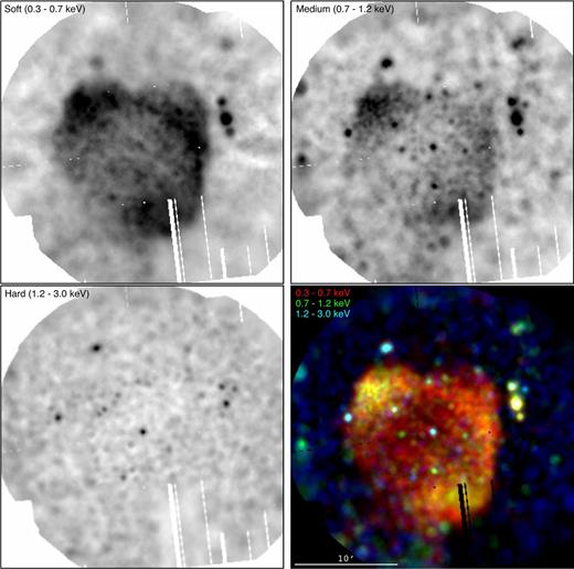
XMM–Newton EPIC (MOS1+MOS1+pn) exposure-corrected X-ray images in three different energy bands of the field of view of NGC 6888. The images in these three energy bands have been combined to produce the colour-composite picture shown in the bottom-right panel. The central star in NGC 6888 (WR 136) is located at the centre of each image. Note that the point sources have not been excised from the observations. North is up, east to the left.
Fig. 1 shows the presence of diffuse X-ray emission towards NGC 6888 as reported by previous works (e.g. Zhekov & Park 2011; Toalá et al. 2014, and references therein) as well as a number of point-like sources in the field of view of the observations including the progenitor star, WR 136. Furthermore, it is clear that the X-ray emission has three maxima associated with the northern and southern caps, and with the north-west blowout detected in [O iii] optical narrowband and Spitzer 24 μm images (see Gvaramadze, Kniazev & Fabrika 2010; Mesa-Delgado et al. 2014).
The diffuse X-ray emission of NGC 6888 shows remarkable spectral variations across the nebula. The bulk emission from the caps and blowout is found in the soft band, with a significant contribution in the medium band. On the other hand, while the central and south-east regions of the nebula are also strong in the soft band, their emission in the medium band is negligible. Furthermore, none of these regions has appreciable emission in the hard band. The differing spatial distribution of the X-ray emission in the soft and medium energy bands hints at spectral differences between regions within the nebula never reported by previous X-ray studies of NGC 6888. Note that no appreciable diffuse X-ray emission is detected in the hard band.
To further illustrate the distribution of the diffuse X-ray emission, we have used the ciaodmfilth routine (ciao version 4.6, Fruscione et al. 2006) to excise all point-like sources and create a clean view of the X-ray-emitting gas in the soft band. The final image is presented in Fig. 2 in comparison with other wavelengths. Fig. 2 – left-hand panel shows the comparison with the H α and [O iii] narrow-band images obtained at the 1 m telescope of the Mount Laguna Observatory (see Gruendl et al. 2000). The X-ray-emitting gas is delimited by the [O iii] skin and not by the H α clumpy distribution. Fig. 2 – right-hand panel shows the comparison of the diffuse X-ray emission with that of the Spitzer 24 μm and H α narrowband emission. The mid-IR emission in the Spitzer 24 μm image also shows a skin at the location of the north-west blowout that confines the diffuse soft X-ray emission.
![X-ray, optical, and mid-IR colour-composite pictures of NGC 6888. Left: H α (red) and [O iii] (green) narrow-band images (Gruendl et al. 2000), and soft (0.3–0.7 keV) diffuse X-ray emission (blue). Right: Spitzer 24 μm (red), H α narrowband image (green), and soft (0.3–0.7 keV) diffuse X-ray emission (blue). The position of the central star, WR 136, is shown in both panels. North is up, east to the left.](https://oup.silverchair-cdn.com/oup/backfile/Content_public/Journal/mnras/456/4/10.1093_mnras_stv2819/3/m_stv2819fig2.jpeg?Expires=1750677677&Signature=hggjZy7N8tU~BCGhh3g1FR5sbuO1utAn9lLXrJCXvP4Pd5ihwCEzMxJMwIUbKPLWnrbJXk4sHGnRd0S0VESCYq-Dr~AwTtkSyZrN7A4rzSowrenpuktRxHt2mSBlhDhfge6o-5UXZuMMJO-0pTJz5qV5yuovmmIv5VyrG3ZblXRa8RK21HElOFOlEbbNiMeGezLc9yxIskAOc7ZbaVMFhL~JsxnL6krLPg7LbtvOqA236EsWdjvaLZAUTMy7JLFFP6p3CooiEttZjafbqWzxbYdM8cQGdwxpHUJ5SZuMj8f5Yc9dg5c4LHa2UqwKQoZsZaiEtqLILuG8j3qAL1p~Vw__&Key-Pair-Id=APKAIE5G5CRDK6RD3PGA)
X-ray, optical, and mid-IR colour-composite pictures of NGC 6888. Left: H α (red) and [O iii] (green) narrow-band images (Gruendl et al. 2000), and soft (0.3–0.7 keV) diffuse X-ray emission (blue). Right: Spitzer 24 μm (red), H α narrowband image (green), and soft (0.3–0.7 keV) diffuse X-ray emission (blue). The position of the central star, WR 136, is shown in both panels. North is up, east to the left.
4 PHYSICAL PROPERTIES OF THE HOT GAS IN NGC 6888
To proceed with the study of the physical properties of the X-ray-emitting gas in NGC 6888, we have extracted X-ray spectra from different regions of this nebula. In order to identify periods of high-background levels, we created light curves binning the data over 100 s for each of the EPIC cameras in the 10–12 keV energy band. Background was considered high for count rate values over 1.0 counts s−1 and 0.2 counts s−1 for the pn and MOS cameras, respectively. The net exposure times after excising bad periods of time are 48.8, 63.8, and 64.9 ks for the pn, MOS1, and MOS2 cameras, respectively.2
In order to study the spectral variations within regions in NGC 6888, we have defined several polygonal apertures as shown in Fig. 3. These apertures delineate specific nebular regions: the north-east (NE) cap, the south-west (SW) cap, the blowout (B), the central region (C), and the southern (S) region. An additional aperture, defined by a source region (shown with red dashed line in Fig. 3) encompassing the [O iii] line emission, correspond to the global diffuse X-ray emission. The background has been extracted from a region close to the camera edges that does not include diffuse X-ray emission from the nebula.
![EPIC-pn event file of the field of view of NGC 6888. The polygonal regions correspond to the source apertures used to extract the spectra, where the circular regions around point-like sources have been excised. The red line encompasses the optical [O iii] emission. The dashed-line polygon shows the region used for the selection of the background region.](https://oup.silverchair-cdn.com/oup/backfile/Content_public/Journal/mnras/456/4/10.1093_mnras_stv2819/3/m_stv2819fig3.jpeg?Expires=1750677677&Signature=JNWyXw3WcC12Hqdt4uQUqWyiSe2ulV~oGy40XCi4qMVXWEgVVXC~52ubO7KEr4jdunvzmxuzDhJ8nvHmAP2oCN75ZaI-4CuLzuUG4k6m4yqoln0amkKlXfYapvNpp4kUfszCpL4zNMSBK-0Tq-Wvlfh59WdfTCP27ZzHDoObzqgNthm5Jn77Q4rvtQrCmcFmPRciNgxLiIpiNB0ZpZnyntYn2izyB7gfXsJkTMetFBXnf5bg6fgY2qzD1BpBEhAnbUZ1g64NJa-XqAk75NYYo4mz8yqxEt5FvoJaCzzkYWbVBQEi4nnhPYXhK8LAmF5eGIkjCIadu1W6FosC6pE8yg__&Key-Pair-Id=APKAIE5G5CRDK6RD3PGA)
EPIC-pn event file of the field of view of NGC 6888. The polygonal regions correspond to the source apertures used to extract the spectra, where the circular regions around point-like sources have been excised. The red line encompasses the optical [O iii] emission. The dashed-line polygon shows the region used for the selection of the background region.
The background-subtracted spectra for the different regions defined above are shown in Fig. 4. The top-left panel of Fig. 4 shows the spectra corresponding to the global X-ray emission in NGC 6888 extracted from the three EPIC cameras (pn, MOS1, and MOS2). For the apertures corresponding to specific nebular regions, we only show the EPIC-pn spectra given the superior quality of these spectra as compared to those extracted from the EPIC-MOS cameras. The final EPIC-pn count rates and count number in the 0.3–1.5 keV for the different regions (NE, SW, blowout, central, and south regions) are presented in the first two columns of Table 1.
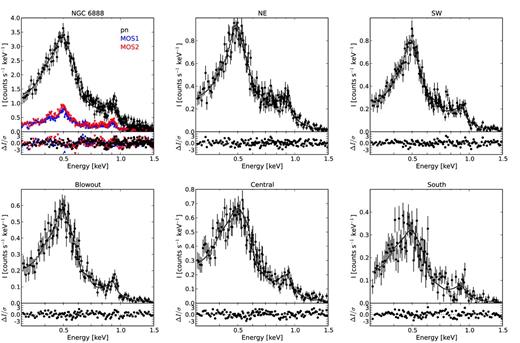
XMM–Newton background-subtracted spectra of different regions of NGC 6888 overplotted with their best-fitting two-temperature apec model shown by solid lines (top panels) and residuals of these fits (bottom panels). The EPIC pn, MOS1, and MOS2 spectra of the whole nebula (top left) are displayed, whereas only the EPIC-pn spectra are shown for specific nebular regions.
Spectral features of the different regions defined in the EPIC-pn observationsa.
| Region | Count rate | Counts | FWHM(E0.5) | R(0.4/0.5)b | R(0.8/0.5)b | R(0.9/0.5)b | R(0.9/0.4)b |
|---|---|---|---|---|---|---|---|
| (counts ks−1) | (keV) | ||||||
| NE | 315 | 14 800±500 | 0.15 | 0.64 | 0.29 | 0.34 | 0.53 |
| SW | 260 | 11 900±200 | 0.14 | 0.61 | 0.27 | 0.27 | 0.43 |
| Blowout | 180 | 8500±150 | 0.19 | 0.65 | 0.18 | 0.22 | 0.34 |
| Central | 250 | 11 600±170 | 0.22 | 0.83 | 0.26 | 0.28 | 0.33 |
| South | 110 | 5050±150 | 0.22 | 1.12 | 0.24 | 0.30 | 0.27 |
aAll values were obtained from EPIC-pn spectra.
bTypical error values are <0.01.
4.1 Spectral Properties
All spectra shown in Fig. 4 are soft and resemble those obtained from Chandra and Suzaku observations (Zhekov & Park 2011; Toalá et al. 2014). The spectra exhibit a broad bump that peaks at 0.5 keV, with a secondary peak at 0.7–1.0 keV. No significant emission is detected at energies above 1.5 keV. The main spectral feature that peaks at 0.5 keV can be associated with the N vii 24.8 Å emission line, while the secondary peak can be attributed to the Fe complex and to Ne ix lines. The spectra in Fig. 4 show subtle differences among them. For example, the 0.5 keV feature of the spectra from the NE and SW regions seem rather narrow, whilst the other regions (blowout, central, and south) show a broader feature.
In order to assess these spectral differences we have calculated the averaged ratio of intensities for different energies. For example, in order to produce the ratio of intensities at 0.4 and 0.5 we have averaged five spectrum channels around each energy value. We have also computed the full width at half-maximum (FWHM) of the emission feature centred at 0.5 keV, FWHM (E0.5). This has been done for each spectra defining a basal value which corresponds to the intensity at 0.8 keV. All these values are presented in Table 1. Column 4 in Table 1 confirms that the feature at 0.5 keV is narrower in the NE and SW spectra than in other regions, with the blowout region having an intermediate value. Furthermore, the ratio between the intensities at 0.4 and 0.5 keV, R(0.4/0.5), shows that the contribution to the 0.4 keV is notably larger in the central and southern regions. In particular, the SW region has the narrowest 0.5 keV spectral feature and the smallest contribution at 0.4 keV, with FWHM(E0.5) = 0.14 keV and R(0.4/0.5) = 0.61.
To finally assure the differences between the background-subtracted spectra, we have run Kolmogorov–Smirnof (KS) statistics tests using the SciPy python library. The KS statistic turned out to be the lowest between the NE and SW spectra, with a value of 0.15. Other KS tests turned out to be higher when comparing the NE (or SW) with spectra from other regions. For example, the KS statistic resulted to be 0.47 when comparing the NE and south region. As lower KS statistics mean that the two samples are more similar, these results prompt us to anticipate that the physical properties between the NE and SW regions will be similar than compared to other regions.
Three different scenarios can be envisaged to interpret these spectral variations: (1) nitrogen abundance variations in different regions, (2) variations in the plasma temperatures, that is, if the caps would have higher temperatures it would produce large emissivity in the N vii line, and (3) higher values of the extinction towards the NE and SE caps would reduce the emission in the lowest energy range.
To study the physical properties of the X-ray emission, all spectra shown in Fig. 4 have been modelled and fit with xspec v12.8.2 (Arnaud 1996), using an absorbed two-temperature apec optically thin plasma emission model with a tbabs absorption model as described in Wilms, Allen & McCray (2000). In accordance with previous X-rays studies of S 308, NGC 2359, and NGC 6888, we use the low temperature component to model the bulk of the X-ray emission, while the higher temperature component models the emission above ∼0.7 keV (Toalá et al. 2012, 2014, 2015a, and references therein). We initially adopted the same nebular abundances as in Toalá et al. (2014) for N, O, and Ne of 3.2, 0.41, and 0.85 times their solar values (Anders & Grevesse 1989), which are averaged values from abundances found by Fernández-Martín et al. (2012) and S abundance of 0.39 times its solar value as found by Moore, Hester & Scowen (2000). Models with variable C, Mg, and Fe were tested but their fitted abundances converged to solar values, so we fixed these abundances. Models with variable Ne were also tested and the final best-fitting values ranged around 0.80 times its solar value. Thus, we kept its value at 0.85 as found by Fernández-Martín et al. (2012). We note that the N/O ratio used here is consistent with those results reported recently by Mesa-Delgado et al. (2014), Stock & Barlow (2014), and Reyes-Pérez et al. (2015).
To evaluate further the three differences scenarios that can cause the spectral differences, we ran different sets of spectral fits varying the nitrogen abundance (XN) and plasma temperatures (kT1 and kT2). Even though extinction has been found to be uniform throughout NGC 6888 by Wendker et al. (1975) and implies a column density of NH = 3.13 × 1021 cm−2 (see Hamann, Wessolowski & Koesterke 1994), we also explore some models with varying hydrogen column density.
The resultant model spectra were compared with the observed spectra in the 0.3–1.5 keV energy range and the χ2 statistics was used to determine the best-fitting models. A minimum of 100 counts per bin was required for the spectral fit. The resultant best-fitting model parameters for all regions are listed in Table 2: plasma temperatures (kT1, kT2), normalization parameters (A1 and A2),3 nitrogen abundance (XN), column density (NH), absorbed and unabsorbed fluxes ( f and F) in the 0.3–1.5 keV energy range, and reduced χ2. We describe these fits in the two following sections.
4.2 Global properties of the hot gas in NGC 6888
To study the global physical properties of NGC 6888 we have fitted the pn, MOS1, and MOS2 spectra simultaneously. For this, we set the column density to a fixed value (NH = 3.13 × 1021 cm−2) and varied the plasma temperatures and nitrogen abundance. The result of this joint fit is given in Table 2 labelled as ‘NGC 6888’. The temperature of the two plasma components are T1 = 1.4 × 10⁶ K (kT1 = 0.120 keV) and T2 = 8.2 × 10⁷ K (kT2 = 0.71 keV), for a nitrogen abundance XN = 3.70 times its solar value. The total absorbed flux is fX = (2.5±0.1) × 10−12 erg cm−2 s−1, which corresponds to an unabsorbed flux of FX = (4.2±0.2) × 10−11 erg cm−2 s−1. Adopting a distance of 1.26 kpc, the X-ray luminosity is LX = (7.9±0.3) × 1033 erg s−1.
Spectral fits of the diffuse X-ray emission from NGC 6888⋆.
| Region | Label | NH | XN/XN, ⊙ | kT1 | |$A_{1}^{\dagger }$| | |$f_{1}^{\ddagger }$| | |$F_{1}^{\ddagger }$| | kT2 | |$A_{2}^{\dagger }$| | |$f_{2}^{\ddagger }$| | |$F_{2}^{\ddagger }$| | F1/F2 | T1/T2 | χ2/DoF |
|---|---|---|---|---|---|---|---|---|---|---|---|---|---|---|
| (×1021 cm−2) | (keV) | (cm−5) | (cgs) | (cgs) | (keV) | (cm−5) | (cgs) | (cgs) | ||||||
| NGC 6888 | #1 | 3.13 | 3.70|$^{+0.23}_{-0.22}$| | 0.120|$^{+0.003}_{-0.002}$| | 5.0 × 10⁻² | 1.9 × 10⁻¹² | 4.1 × 10⁻¹¹ | 0.71|$^{+0.02}_{-0.02}$| | 6.1 × 10⁻⁴ | 5.9 × 10⁻¹³ | 1.8 × 10⁻¹² | 22.2 | ... | 1.45 = 874.88/600 |
| EPIC-pn | #1 | 3.13 | 3.75|$^{+0.35}_{-0.32}$| | 0.122|$^{+0.004}_{-0.003}$| | 4.6 × 10⁻² | 2.0 × 10⁻¹² | 3.9 × 10⁻¹¹ | 0.74|$^{+0.03}_{-0.03}$| | 6.0 × 10⁻⁴ | 5.8 × 10⁻¹³ | 1.7 × 10⁻¹² | 22.4 | ... | 1.30 = 307.24/241 |
| #2 | 3.13 | 4.0 | 0.123|$^{+0.003}_{-0.003}$| | 4.3 × 10⁻² | 2.0 × 10⁻¹² | 3.8 × 10⁻¹¹ | 0.74|$^{+0.03}_{-0.03}$| | 6.1 × 10⁻⁴ | 5.9 × 10⁻¹³ | 1.8 × 10⁻¹² | 21.1 | ... | 1.32 = 314.08/237 | |
| NE | #1 | 3.13 | 4.72|$^{+0.71}_{-0.95}$| | 0.139|$^{+0.004}_{-0.014}$| | 7.9 × 10⁻³ | 5.6 × 10⁻¹³ | 9.3 × 10⁻¹² | 0.73|$^{+0.05}_{-0.04}$| | 1.8 × 10⁻⁵ | 1.8 × 10⁻¹³ | 5.5 × 10⁻¹³ | 16.8 | 0.19 | 1.14 = 214.35/188 |
| #2 | 3.13 | 4.0 | 0.129|$^{+0.007}_{-0.005}$| | 1.0 × 10⁻² | 5.3 × 10⁻¹³ | 9.8 × 10⁻¹² | 0.71|$^{+0.03}_{-0.05}$| | 2.0 × 10⁻⁴ | 1.9 × 10⁻¹³ | 5.9 × 10⁻¹³ | 16.7 | 0.18 | 1.15 = 187.60/163 | |
| #3 | 3.70|$^{+0.27}_{-0.26}$| | 4.0 | 0.120 | 1.9 × 10⁻² | 5.4 × 10⁻¹³ | 1.7 × 10⁻¹¹ | 0.71 | 2.2 × 10⁻⁴ | 1.8 × 10⁻¹³ | 8.0 × 10⁻¹³ | 20.3 | 0.17 | 1.14 = 187.16/164 | |
| SW | #1 | 3.13 | 5.50|$^{+1.00}_{-0.80}$| | 0.143|$^{+0.005}_{-0.004}$| | 6.8 × 10⁻³ | 5.6 × 10⁻¹³ | 8.9 × 10⁻¹² | 0.78|$^{+0.08}_{-0.07}$| | 1.3 × 10⁻⁴ | 1.3 × 10⁻¹³ | 3.8 × 10⁻¹³ | 22.9 | 0.18 | 0.97 = 178.40/184 |
| #2 | 3.13 | 4.0 | 0.130|$^{+0.009}_{-0.006}$| | 1.0 × 10⁻² | 5.4 × 10⁻¹³ | 9.9 × 10⁻¹² | 0.72|$^{+0.04}_{-0.06}$| | 1.7 × 10⁻⁴ | 1.6 × 10⁻¹³ | 4.9 × 10⁻¹³ | 20.1 | 0.18 | 1.03 = 149.75/145 | |
| #3 | 3.85|$^{+0.32}_{-0.31}$| | 4.0 | 0.120 | 2.3 × 10⁻² | 5.9 × 10⁻¹³ | 1.9 × 10⁻¹¹ | 0.71 | 1.8 × 10⁻⁴ | 1.1 × 10⁻¹³ | 7.0 × 10⁻¹³ | 27.1 | 0.17 | 1.00 = 144.62/146 | |
| Blowout (B) | #1 | 3.13 | 3.85|$^{+0.65}_{-0.55}$| | 0.125|$^{+0.008}_{-0.006}$| | 7.6 × 10⁻³ | 3.5 × 10⁻¹³ | 6.8 × 10⁻¹² | 0.80|$^{+0.09}_{-0.08}$| | 6.3 × 10⁻⁵ | 6.3 × 10⁻¹⁴ | 1.8 × 10⁻¹³ | 37.4 | 0.16 | 0.98 = 117.16/119 |
| #2 | 3.13 | 4.0 | 0.126|$^{+0.007}_{-0.005}$| | 7.3 × 10⁻³ | 3.5 × 10⁻¹³ | 6.7 × 10⁻¹² | 0.80|$^{+0.09}_{-0.08}$| | 6.4 × 10⁻⁵ | 6.3 × 10⁻¹⁴ | 1.8 × 10⁻¹³ | 36.7 | 0.15 | 0.98 = 117.31/120 | |
| #3 | 3.4|$^{+0.32}_{-0.31}$| | 4.0 | 0.120 | 1.1 × 10⁻² | 3.6 × 10⁻¹³ | 9.4 × 10⁻¹² | 0.71 | 6.3 × 10⁻⁵ | 5.4 × 10⁻¹⁴ | 1.8 × 10⁻¹³ | 52.3 | 0.17 | 0.98 = 118.88/121 | |
| Central (C) | #1 | 3.13 | 2.90|$^{+0.51}_{-0.50}$| | 0.115|$^{+0.005}_{-0.004}$| | 1.2 × 10⁻² | 3.7 × 10⁻¹³ | 8.2 × 10⁻¹² | 0.78|$^{+0.05}_{-0.05}$| | 1.1 × 10⁻⁴ | 1.0 × 10⁻¹³ | 3.0 × 10⁻¹³ | 27.0 | 0.15 | 1.35 = 185.31/137 |
| #2 | 3.13 | 4.0 | 0.121|$^{+0.006}_{-0.004}$| | 8.5 × 10⁻³ | 3.6 × 10⁻¹³ | 7.3 × 10⁻¹² | 0.77|$^{+0.05}_{-0.05}$| | 1.0 × 10⁻⁴ | 1.0 × 10⁻¹³ | 3.1 × 10⁻¹³ | 23.7 | 0.15 | 1.42 = 196.62/138 | |
| #3 | 3.04|$^{+0.32}_{-0.29}$| | 4.0 | 0.120 | 8.1 × 10⁻³ | 3.6 × 10⁻¹³ | 6.8 × 10⁻¹² | 0.71 | 1.0 × 10⁻⁴ | 1.0 × 10⁻¹³ | 3.2 × 10⁻¹³ | 21.3 | 0.17 | 1.45 = 201.93/139 | |
| South (S) | #1 | 3.13 | 3.71|$^{+1.20}_{-0.90}$| | 0.113|$^{+0.008}_{-0.008}$| | 5.7 × 10⁻³ | 1.9 × 10⁻¹³ | 4.2 × 10⁻¹² | 0.79|$^{+0.13}_{-0.14}$| | 4.2 × 10⁻⁵ | 4.1 × 10⁻¹⁴ | 1.2 × 10⁻¹³ | 35.0 | 0.14 | 1.17 = 186.76/159 |
| #2 | 3.13 | 4.0 | 0.115|$^{+0.007}_{-0.006}$| | 5.2 × 10⁻³ | 1.8 × 10⁻¹³ | 4.1 × 10⁻¹² | 0.78|$^{+0.13}_{-0.15}$| | 4.3 × 10⁻⁵ | 4.2 × 10⁻¹⁴ | 1.2 × 10⁻¹³ | 33.2 | 0.15 | 1.23 = 145.33/118 | |
| #3 | 2.71|$^{+0.53}_{-0.46}$| | 4.0 | 0.120 | 3.2 × 10⁻³ | 1.8 × 10⁻¹³ | 2.7 × 10⁻¹² | 0.71 | 3.9 × 10⁻⁵ | 4.4 × 10⁻¹⁴ | 1.5 × 10⁻¹³ | 18.0 | 0.17 | 1.22 = 145.68/119 |
⋆Boldface text represent fixed values on each fit.
†The normalization parameter is defined as |$A = 1 \times 10^{-14} \int n_\mathrm{e} n_\mathrm{H} {\rm d}V/ 4 \pi d^{2}$|, where d, ne, nH, and V are the distance, electron and hydrogen number densities, and volume in cgs units, respectively.
‡Fluxes ( f and F) are computed in the 0.3–1.5 keV energy range and are presented in cgs units (erg cm−2 s−1).
In order to estimate the electron density of the X-ray-emitting gas, we can assume a spherical morphology (see Toalá et al. 2014, for a discussion on adopting different morphologies). At a distance of 1.26 kpc the maximum extent of the nebula, that is 9 arcmin, represents a physical radius of 3.3 pc. Using the definition of the normalization parameter (A), we can estimate an electron density of ne = 0.4(ϵ/0.1)−1/2 cm−3, which implies a mass of mX = 1.7(ϵ/0.1)1/2 M⊙, with ϵ as the filling factor. Note that these values are the same as those estimated from the Chandra observations which only covered ∼60 per cent of the nebula (see Toalá et al. 2014).
The reduced χ2 of the above fit is good, but not optimal (1.45). This implies that there is an underlying complexity to the emitted spectrum, exceeding the simple model here proposed, but it may point also to calibration discrepancies among the three EPIC cameras. To investigate this issue, we also performed model fits to the data of NGC 6888 obtained solely from the EPIC-pn camera. The best-fitting model parameters to this emission are also shown in Table 2 labelled as 'EPIC-pn #1’. The model delivered similar temperatures for the plasma, T1 = 1.4 × 10⁶ K and T2 = 8.6 × 10⁷ K, and a nitrogen abundance of XN = 3.75 times its solar value. The corresponding total absorbed and unabsorbed fluxes are fX = (2.6±0.2) × 10−12 erg cm−2 s−1 and FX = (4.1±0.3) × 10−11 erg cm−2 s−1. The corresponding luminosity is LX = (7.8±0.6) × 1033 erg s−1. One more model (#2) was tested by fixing the nitrogen abundance XN = 4, but similar results were obtained (see Table 2). The reduced χ2 of the fits to the EPIC-pn spectrum is somewhat lowered (1.3), but still significantly above unity.
4.3 Physical properties of the different regions
In order to study the variations of the physical conditions in the plasma within NGC 6888, we have modelled separately the different spectra as extracted from different regions defined in Fig. 3 as NE, SW, blowout, central, and south. We have tried three types of models: (1) in models labelled as #1 only the column density has been set to the fixed nominal value NH = 3.13 × 1021 cm−2, (2) for models labelled as #2 both the column density and the nitrogen abundance have been fixed (NH = 3.13 × 1021 cm−2 and XN = 4), finally 3) in models labelled as #3, the nitrogen abundance and plasma temperatures have been fixed to those values obtained from the global fit of NGC 6888 using the three EPIC cameras (XN = 4, kT1 = 0.120 keV, and kT2 = 0.71 keV), but the hydrogen column density has been set as a free parameter of the model. The results are shown in Table 1.
The spectral fits obtained using the models mentioned above are generally consistent with those found for the global spectra derived from the three EPIC cameras and from the pn camera, although there is evidence for variations in the plasma properties. The reduced χ2 are improved in the spectral fits, except for the central region. The temperature of the main plasma component in the NE and SW regions (T1 ∼1.6 × 10⁶ K; models NE#1, NE#2, SW#1, and SW#2) seems to be a bit higher than in other regions (T1 ≲1.4 × 10⁶ K; models B#1, B#2, C#1, and C#2). On the other hand, the temperature of the second component (T2 = 8–9 × 10⁶ K) is consistent among the different regions, within the error bars. Models labelled as #1 provide hints of enhanced nitrogen abundances in the NE and SW regions, with nitrogen abundances somewhat higher (XN ∼ 5) than in other regions (XN < 3.9). Alternatively, models labelled as #3 suggest that the NE and SW spectra are more extinguished than the spectra extracted from other regions. These detailed fits thus confirm the spectral differences seen in Fig. 1 and revealed in Table 1.
5 DISCUSSION
The WR nebula NGC 6888 received attention from almost all previous X-ray telescopes, such as Einstein, ROSAT, ASCA, Suzaku, and Chandra, but this is the first time that it has been mapped entirely at high sensitivity with reasonable spatial resolution (∼6 arcsec). In general, the spatial distribution of the X-ray emission resulting from the current XMM–Newton observations is in agreement with previous results, although the X-ray images in Figs 1 and 2 reveal structures in great detail. The morphology of the X-ray emission of NGC 6888 is far from simple: most emission comes from three maxima at the north-east and south-west caps and north-west blowout, while the central and south-western regions show a rather homogeneous distribution of the X-ray emitting gas. The X-ray emission from the north-west region is confined by the north-west blowout delineated by optical [O iii] and Spitzer 24 μm emission.
Previous X-ray observations of NGC 6888 did not have the capabilities of resolving spectral differences across the nebula, consequently only its global properties could be derived. The Chandra observations of NGC 6888 presented by Toalá et al. (2014) hinted at the presence of spatial variations in the spectral properties of its diffuse X-ray emission, but the differing spectral responses at low energies of the two Chandra ACIS-S CCDs that registered this emission cast uncertainties on this finding. The unprecedented sensitivity, full spatial coverage and homogeneous spectral response of the current observations enabled the search for unambiguous spatial variations in the spectral properties of the diffuse X-ray emission from NGC 6888. This resulted in the conclusive detection of spectral differences at different locations of a WR nebula for the first time. These are clearly revealed in Figs 1 and 4 and corroborated by Tables 1 and 2.
In order to assess the origin of the spectral differences and explore the three possible scenarios proposed in Section 4.1, we have performed different fits to each of them labelled as #1, #2, and #3 (see Section 4.3). In particular, models labelled as #2 provided a clear support for variations of the main plasma temperature, kT1, of the caps with respect to the remaining regions, from |$(1.5^{+0.10}_{-0.06})\times 10^{6}$| K in the caps down to |$(1.3^{+0.08}_{-0.07})\times 10^{6}$| K in the central and southern regions. This trend is confirmed by the best-fitting parameters of models #1, that suggest both nitrogen abundances enhancements, up to XN ∼ 5, and larger plasma temperatures at the caps with respect to the central and southernmost regions, with XN < 3.9. With models labelled as #3 we wanted to assess the possible variations of the absorption column density. The best-fitting parameters of the latter models suggest that the NE and SW regions (the caps) have slightly larger NH, but the extinction variations among the different regions, all within the error bars, are not conclusive. Furthermore, if column density variations were the reason for the differences in the spectra shown in Fig. 4 we would have expected larger values towards the central and south regions as suggested by the Herschel PACS 160 μm image of NGC 6888 (Toalá et al., in preparation). Finally, we would like to mention that in all different fits, the blowout region shows intermediate values of plasma temperature and nitrogen abundances.
The above spectral analysis leads us to conclude that the diffuse X-ray emission from NGC 6888 is not affected by significant extinction variations, but rather it indicates correlated variations in the plasma temperatures and nitrogen abundances. Regions with lower plasma temperatures (i.e. the central and southern regions) have nitrogen abundances closer to those of the optical nebula (e.g. Reyes-Pérez et al. 2015), whereas regions with higher plasma temperatures (i.e. the caps) have higher nitrogen abundances. These correlations can be interpreted as evidence of low mixing efficiency between the stellar wind and the nebular material in the caps. In other words, the higher temperature of the NE and SW regions implies less mixing with the outer nebular material.
It could be argued that the contrasting mixing efficiency across the nebula is caused by the presence of a magnetic field which would suppress thermal conduction in the direction perpendicular to the magnetic lines. At this time, however, there is no definitive detection of magnetic fields in WR 136 (e.g. Kholtygin et al. 2011; de la Chevrotière et al. 2014) or its associated nebula (Wendker et al. 1975). The physical structure of NGC 6888 and its surrounding medium offer alternative explanations. The nebula seems to be located at the edge of a cold cloud revealed by its infrared emission (see Gvaramadze et al. 2010). This is illustrated by the Spitzer 24 μm emission from the nebula and its surrounding medium shown in red in the right-hand panel of Fig. 2. The spatial coincidence between the 24 μm emission from the nebula and the H α emission from clumps and filaments and the [O iii] emission from the blowout suggests a contribution of ionized material to the nebular emission in this band and a contribution by thermal dust emission (e.g. Toalá et al. 2015b). The lack of mid-IR emission towards the north-west of the WR bubble reveals the low density of the ISM along this direction, naturally explaining the production of the blowout. On the other hand, the caps are formed as the stellar wind of the WR star sweeps up material along directions of higher density. The anisotropic of the ISM around WR 136 can be expected to produce different shock structures, depending on the density of the surrounding material. These would result in different types of hydrodynamical instabilities with varying efficiencies in the injection and mixing of cold nebular material into the hot bubble along different directions.
5.1 Comparison with other Wolf–Rayet nebulae
Currently, there are three WR bubbles that have been reported to harbour diffuse X-ray emission, namely, S 308, NGC 2359, and NGC 6888 around WR 6, WR 7, and WR 136, respectively. The best-quality observations of these WR bubbles, those performed by XMM–Newton (Chu et al. 2003; Toalá et al. 2012, 2015a, this work), suggest different scenarios for their formation.
The simplest case would be that of the WR nebula around WR 6, S 308. The H i distribution around the nebula (Arnal & Cappa 1996) indicates that the dense and slow wind material previous to the WR phase was ejected into a low-density cavity, probably carved by the stellar feedback during the time the star was on the MS phase. Moreover, radiative-hydrodynamic simulations require WR 6 to evolve through a yellow supergiant stage, with correspondingly high dense wind velocities 75 km s−1 (Humphreys 2010), in order to produce a WR bubble of radius as large as that of S 308, ∼9 pc (Toalá & Arthur 2011). As a result, the stellar wind during the subsequent WR phase swept smoothly the previous dense material into a roundish morphology.
Meanwhile, the WR bubble NGC 2359 around WR 7 presents a more complex morphology, with a main bubble and several filaments and blisters (see figs 1 and 3 in Toalá et al. 2015a). X-ray-emitting gas is detected towards the central cavity and inside the north-east blister, with no emission detected towards the southern blister due to high extinction at this region (Toalá et al. 2015a, and references therein). These features are suggestive of the evolution of WR 7 through eruptive and non-isotropic ejections of dense material in an LBV episode (e.g. Rizzo, Martín-Pintado & Desmurs 2003), but also reveal a complex CSM around WR 7.
Finally, NGC 6888 presents a clear case of the formation of a WR bubble in a highly anisotropic CSM. The added complexity of the CSM produces varying interactions of the fast stellar wind along different directions resulting in anisotropic distributions of the plasma temperature and abundances of the X-ray-emitting material.
The detection of X-ray emission inside these three WR bubbles and the non-detections in RCW58 and the WR nebula around WR 16 (Gosset et al. 2005; Toalá & Guerrero 2013) are revealing. Despite the different scenarios for the formation of the three X-ray-emitting WR nebulae, their central stars share similar spectral types and wind properties (WN4–6, v∞ ≈ 1700 km s−1, and |$\dot{M} \approx 5\times 10^{-5}$| M⊙ yr−1, see Hamann, Gräfener & Liermann 2006). These properties are at variance with those of the WR stars whose wind-blown bubbles are not detected in X-rays: WN8h stars with similarly high mass-loss rates, but lower stellar wind velocities v∞ = 650 km s−1 (Hamann et al. 2006).
The current X-ray observations towards WR nebulae suggest that weak stellar winds are not capable of producing diffuse X-ray emission. The theory of wind-blown bubbles predicts that the current fast stellar wind from the central star will ram on to the nebular material producing an adiabatically shocked region, the so-called hot bubble, with temperatures as high as 107–108 K (see Dyson & Williams 1997). We remark that this theoretical prediction is expected even for stellar wind velocities as low as 650 km s−1. The low X-ray temperatures (T ∼ 106 K) implied by the XMM–Newton observations of WR bubbles suggest that the hot plasma inside these bubbles results from the mixing between shocked stellar wind and nebular material due to instabilities formed in the wind–wind interaction zone and/or thermal conduction by hot electrons (e.g. Freyer, Hensler & Yorke 2006; Toalá & Arthur 2011; Dwarkadas & Rosenberg 2013, and references therein). Somehow, weak stellar winds cannot enhance the mixing between the outer ionized material and the shocked stellar wind and, thus, their WR nebulae do not exhibit diffuse X-ray emission. New physical processes (e.g. dust cooling, anisotropic CSM,...) need to be incorporated into theoretical simulations to provide a realistic description of the observations.
6 SUMMARY
This work presents XMM–Newton observations of the WR bubble NGC 6888 around WR 136. We have completed a high-spatial resolution mapping of the nebula for the first time. This has allowed us to corroborate the Toalá et al. (2014) suggestion that the diffuse X-ray emission fills the north-west blowout. The diffuse X-ray emission fills the [O iii] emission and is not only spatially related to the inner H α clumpy distribution as suggested by previous authors. The complex distribution of the X-ray-emitting gas within the WR bubble, as well as the distribution of ionized gas and the outer infrared emission seem to point out that the formation scenario of NGC 6888 is not as simple as that proposed by the classic wind–wind interaction model (e.g. Garcia-Segura et al. 1996a,b; Freyer et al. 2006; Toalá & Arthur 2011).
The uniquely high count rate obtained from the present observations allows a detailed study of the spectral variations across the nebula for the first time. Five different regions have been identified in the X-ray emission: two associated with the caps seen in optical and infrared images and one with the blowout, one to the central region, and one to the southern region. Our analysis suggests that the caps have suffered less mixing of material from the nebula, having higher temperatures and higher nitrogen abundance than those from other regions. The other regions exhibit lower plasma temperatures and lower nitrogen abundances, closer to the nebular abundances, i.e. the mixing has been more efficient. Such variations could be due to the presence of a magnetic field (not reported to date) or to different shock patterns created by the interaction of the stellar wind of WR 136 with the inhomogeneous CSM around NGC 6888.
The total unabsorbed X-ray flux in the 0.3–1.5 keV energy band is estimated to be FX = (4.2±0.2) × 10−11 erg cm−2 s−1 which corresponds to a luminosity of LX = (7.9±0.3) × 1033 erg s−1 at a distance of 1.26 kpc. The rms electron density was estimated to be ne = 0.4(ϵ/0.1)−1/2 which results in a total mass of the X-ray-emitting gas of mX = 1.7(ϵ/0.1)1/2 M⊙, with ϵ as the gas filling factor.
This work was based on observations obtained with XMM–Newton, an ESA science mission with instruments and contributions directly funded by ESA Member States and NASA.
MAG and JAT are supported by the Spanish MICINN (Ministerio de Ciencia e Innovación) grants AYA 2011-29754-C03-02 and AYA 2014-57280-P. SJA and JAT acknowledge financial support through PAPIIT project IN101713 from DGAPA-UNAM (Mexico).
The online version of the XMM-ESAS cookbook can be found at ftp://xmm.esac.esa.int/pub/xmm-esas/xmm-esas.pdf
Note the differences in the net exposure times between the esas tasks and this procedure (see also Toalá et al. 2015a, for the case of NGC 2359).
The normalization parameter is defined as A = 1 × 10− 14∫nenH dV/4πd2, where d is the distance, nH and ne are the number hydrogen and electron density, respectively, and V the volume in cgs units.
REFERENCES
