


Abstract
We have selected a sample of extremely isolated galaxies (EIGs) from the local Universe (z < 0.024), using a simple isolation criterion: having no known neighbours closer than 300 km s−1(3 h−1 Mpc) in the three-dimensional redshift space (α, δ, z). The sample is unique both in its level of isolation and in the fact that it utilizes H i redshifts from the Arecibo Legacy Fast ALFA (ALFALFA) survey. We analysed the EIG sample using cosmological simulations and found that it contains EIGs with normal mass haloes which have evolved gradually with little or no ‘major events’ (major mergers, or major mass-loss events) in the last 3 Gyr. The fraction of EIGs which deviate from this definition (false positives) is 5–10 per cent. For the general population of dark matter haloes, it was further found that the mass accretion (relative to the current halo mass) is affected by the halo environment mainly through strong interactions with its neighbours. As long as a halo does not experience major events, its mass accretion history does not depend significantly on its environment. ‘Major events’ seem to be the main mechanism that creates low-mass subhaloes (Mhalo < 1010 h− 1 M⊙) that host galaxies (with Mg ≲ −14).
1 INTRODUCTION AND BACKGROUND
The research described here is part of an extensive study of star formation properties and evolution of galaxies in different environments and of various morphological types, conducted in the past few decades (e.g. Brosch 1983; Almoznino 1995; Almoznino & Brosch 1998; Brosch, Heller & Almoznino 1998; Heller 2001; Weingarten 2003; Brosch et al. 2008; Zitrin & Brosch 2008). Specifically, we studied galaxies in the most extremely underdense regions of the local Universe. These galaxies are particularly interesting since they evolved with little or no environmental interference, and are therefore useful for validating and calibrating galaxy evolution models. Furthermore, when compared to galaxies in denser regions, they illuminate the overall effects of the environment on the evolution of galaxies.
We have chosen a sample of extremely isolated galaxies (EIGs) from the local Universe (z < 0.024), based on a simple isolation criterion. The neighbourhood properties of this sample were analysed in detail using both observational data and cosmological simulations. The cosmological simulations were further used to estimate the properties and histories of the dark matter (DM) haloes in which the sample EIGs reside.
One of the unique advantages of the EIG sample we study here is that, apart from the optical redshift data commonly used to estimate environment density, it also utilized H i redshifts from the Arecibo Legacy Fast ALFA (ALFALFA) survey (Haynes et al. 2011). The ALFALFA survey is a second-generation untargeted extragalactic H i survey initiated in 2005 (Giovanelli et al. 2005, 2007; Saintonge 2007). This survey utilizes the superior sensitivity and angular resolution of the Arecibo 305 m radio telescope to conduct the deepest ever census of the local H i Universe. ALFALFA was particularly useful in verifying the isolation of the target galaxies, since by being an H i survey it easily measures redshifts of low surface brightness galaxies and other low-luminosity late-type neighbours that are often difficult to detect optically but abound with H i.
When analysing the neighbourhood content, one should not ignore the possible presence of large invisible masses near the target galaxy. These ‘dark haloes’ or ‘dark galaxies’ can be composed of dark as well as non-luminous baryonic matter. Such dark galaxies with masses up to 1011 M⊙ might exist (Tully 2005), and their number density may be comparable to or even exceed by an order of magnitude that of luminous galaxies (Klypin et al. 1999). Karachentsev, Karachentseva & Huchtmeier (2006) estimated that the density of dark galaxies is less than ∼1/20 of the population of luminous galaxies. This estimate came from a search for effects of interactions with neighbouring galaxies in some 1500 isolated galaxies (IGs). They found that no more than 0.3 per cent of the IGs were disturbed to a noticeable level by dark galaxies. If a dark galaxy contains sufficient H i, it might be detected by ALFALFA. In the latest ALFALFA catalogue (α.40; Haynes et al. 2011), 199 such dark galaxies were found. Many of these are suspected to be tidal or ram-pressure debris of nearby galaxies (e.g. Koopmann et al. 2008). ALFALFA is, therefore, an extremely important tool for testing the isolation of galaxies.
Extensive optical imaging of the sample EIGs in broad-band and rest-frame Hα was performed using the Wise Observatory1 (WO) 1 m telescope. This, along with public observational data, was used to measure the current star formation (following the method described in Spector, Finkelman & Brosch 2012) and to estimate its history. These observational results will be described and discussed in detail in Spector & Brosch (in preparation).
This work attempts, among other things, to help resolve the question of ‘Nature versus Nurture’: does the evolution of galaxies depend only on their content or do their large-scale environments have a significant evolutionary influence. Some argue that galaxy formation is driven predominantly by the mass of the host DM halo, and is nearly independent of the larger scale halo environment (e.g. Croton & Farrar 2008; Tinker & Conroy 2009). This is supported by their simulation models that produce void galaxies conforming to some observed statistical properties. However, since there are many galaxy properties that current simulations cannot predict, and since the halo mass of galaxies cannot be directly measured, this hypothesis is hard to prove or disprove.
For similar purposes, other samples of IGs were defined and studied in ‘the Analysis of the interstellar Medium of Isolated GAlaxies’ (AMIGA) international project (Verley et al. 2007; Fernández Lorenzo et al. 2013), in the ‘Two Micron Isolated Galaxy’ (2MIG) catalogue (Karachentseva et al. 2010), in the ‘Local Orphan Galaxies’ (LOG) catalogue (Karachentsev et al. 2011, 2013) and in the Void Galaxy Survey (VGS; Kreckel et al. 2012). These are discussed in Section 2.5.
In Section 2, the method used for selecting the sample of EIGs is described, the sample galaxies are listed, and their observed neighbourhoods are discussed and compared to those of other IG surveys. Section 3 describes how cosmological simulations were used to analyse the EIG sample, and discusses the estimated halo properties and histories of the EIGs, as well as the properties of their neighbourhoods.
Throughout this work, unless indicated otherwise, Λ cold dark matter (ΛCDM) cosmology with the seven-year Wilkinson Microwave Anisotropy Probe data (WMAP7; Bennett et al. 2011) parameters are used, including the dimensionless Hubble parameter h = 0.704. We adopt here the solar g-band absolute magnitude of Mg,⊙ = +5.12 (according to the Sloan Digital Sky Survey, SDSS, DR7 website2).
2 THE SAMPLE
The first and possibly most crucial step in this study is selecting a sample of galaxies in extremely underdense regions, referred to here as EIGs. By definition, these EIGs are very rare and, therefore, at moderate redshifts the sample is expected to be fairly small, including only a few dozen galaxies. This section describes the method used for selecting the sample, lists the sample galaxies, discusses their observed neighbourhoods and compares these with other IG catalogues.
2.1 Isolation criterion
In the last few decades, great advances were made in redshift surveys, which now map the local Universe in redshift space with great precision. Before these became available, IGs had to be identified using projected coordinates alone, i.e. searching in two-dimensional (2D) space. Radial distances had to be estimated, for example, using the angular sizes of galaxies, such as done for the classical Catalogue of Isolated Galaxies (CIG; Karachentseva 1973) and in Karachentseva et al. (2010).
The use of redshift data for testing the isolation of galaxies started decades ago (Huchra & Thuan 1977). Nowadays, when the local Universe is mapped in detail, it is possible to perform accurate three-dimensional (3D) redshift space searches. The advantages of using such strategy are simplicity and straightforwardness, not having to assume anything about the characteristics of the galaxies (size, magnitude, etc.).
However, using redshift mapping introduces two difficulties. First is the incompleteness of most redshift data bases. A galaxy that seems to be isolated might have neighbours for which a redshift was not yet measured. Second is the error in radial distance introduced by peculiar velocities. Using redshift data one performs a search in 3D redshift space, the mathematical representation of the projected coordinates: right ascension (α) and declination (δ) and the radial coordinate: redshift (z). It should be kept in mind that mapping in 3D redshift space (α, δ, z) can differ significantly from the true mapping in real space. For example, although close in real space, two galaxies in a cluster might have very different redshifts due to the cluster velocity dispersion and will therefore seem distant in 3D redshift space.
In principle, independent distance measurements (not based on redshift measurements) have the potential to improve uncertainties caused by peculiar velocities. Currently, independent distance measurements are available for more than 8000 galaxies in the local Universe. These were used by Tully et al. (2014) to find the limits of the ‘Laniakea’ supercluster in which we live. The accuracy of these distance measurements for very close galaxies and for early-type galaxies (typically located in dense regions) is ∼10 per cent, while the accuracy for the more distant late types (typically located in isolated regions) is ∼20 per cent (Courtois et al. 2012). When averaged, these give sufficient accuracy to map cosmic flows. However, for testing the isolation of individual galaxies in the redshift range of this research, these independent distance measurements are not accurate enough.
In this work, we have chosen to use the simple isolation criterion described in Spector & Brosch (2010). A galaxy is considered an EIG and is included in the sample if it has no known neighbours closer than 300 km s−1 in 3D redshift space, and if its redshift is in the range 2000 < cz < 7000 km s−1. This translates to not having any known neighbour within a distance of 3 h−1 Mpc ≅ 4.26 Mpc.3
The redshift range was limited to 7000 km s−1 to have reasonable completeness of redshift data around each galaxy. The reason for the lower limit of 2000 km s−1 is to keep the sky area that has to be searched around each galaxy relatively small, since at 2000 km s−1 neighbours have to be searched for as far as 8.6° away.
No magnitude, H i mass, or size limit was used in the selection of candidate neighbours. The use of such limits would have somewhat reduced the level of isolation of the sample (especially for the closer EIGs), and therefore was not preferred. Not using such limits, however, complicates somewhat the analysis of the sample's isolation level (described in Section 3).
2.2 Selection process
The search criterion was applied to two sky regions, one in the spring sky (Spring) and the other in the autumn sky (Autumn), as described in Table 1. These particular regions were selected since they are covered by the α.40 ALFALFA catalogue (Haynes et al. 2011). Both regions include mainly high Galactic latitudes. The Spring region is almost fully covered by spectroscopic data in SDSS DR10 (Ahn et al. 2014).
Sample search regions.
| α (J2000) | δ (J2000) | cz (km s−1) | Volume (h−3 Mpc3) | |
|---|---|---|---|---|
| Spring | 7h30m–16h30m | 4°–16° | 2000–7000 | 5.42 × 10⁴ |
| Autumn | 22h00m–03h00m | 24°–28° | 2000–7000 | 9.17 × 10³ |
| α (J2000) | δ (J2000) | cz (km s−1) | Volume (h−3 Mpc3) | |
|---|---|---|---|---|
| Spring | 7h30m–16h30m | 4°–16° | 2000–7000 | 5.42 × 10⁴ |
| Autumn | 22h00m–03h00m | 24°–28° | 2000–7000 | 9.17 × 10³ |
The Spring region contains parts of the following large-scale structures (ordered by increasing redshift): Virgo cluster, Virgo void, Coma void, Microscopium void and the Coma wall. The Autumn region contains parts of the following large-scale structures (ordered by increasing redshift): Delphinus void, Taurus void, Eridanus void, Perseus Pisces supercluster, Pegasus void and Pisces void (Fairall 1998).
To allow searching for neighbours near the edges of the these search regions, larger data base regions were used. The region downloaded from the NASA/IPAC Extragalactic Database4 (NED) for the Spring region was 6h40m < α < 17h20m, −8° < δ < 28°, 1600 < cz < 7400 km s−1. The region downloaded from NED for the Autumn region was 21h00m < α < 04h00m, 12° < δ < 40°, 1600 < cz < 7400 km s−1. These regions allow searching for neighbours at distances of up to 400 km s−1 (equivalent to 4 h−1 Mpc) from the candidate galaxies.
Data for these regions were downloaded from NED on 2012 November 13. The NED object types included in the data base were galaxies, galaxy clusters, galaxy pairs, galaxy triples, galaxy groups and QSO. The Spring data base region included 14,273 objects, while the Autumn data base region included 3956 objects.
The ALFALFA data base used was the ‘α.40 H i source catalogue’ (α.40; Haynes et al. 2011). This catalogue covers 40 per cent of the final ALFALFA survey area (∼2800 deg2) and contains 15,855 sources. It includes parts of the required Spring region: |$ {07^{\rm h} 30^{\rm m}} < {\alpha } < {16^{\rm h}30^{\rm m}}$|, +04° < δ < +16° and +24° < δ < +28°, and parts of the required Autumn region: |${22^{\rm h}} < {\alpha } < {03^{\rm h}}$|, +14° < δ < +16° and +24° < δ < +32°. The data base covers the required redshift range (1600 < cz < 7400 km s−1).
For each EIG found in these searches, the NED redshift measurement was verified by comparing it to ALFALFA, SDSS DR10 and all sources quoted by NED. The redshift values adopted here for the EIGs were chosen based on the following priority list.
If an optically derived redshift value with uncertainty <10 km s−1 exists, it was adopted. If several such values exist, the SDSS value of the latest available data release (usually DR10) was preferred.
Otherwise, if a 21 cm redshift value with uncertainty <10 km s−1 exists, it was adopted. If several such values exist, the ALFALFA value was preferred.
Otherwise, if reasonably accurate redshift values exist (Δcz < 30 km s−1), the most accurate of them was adopted.
If no reasonably accurate value exists (i.e. Δcz ≥ 30 km s−1), the galaxy was deleted from the sample.
Optical redshift measurements were preferred because they are expected to be more accurate for estimating the transmittance of the Hα filters in the redshifted Hα line.
The EIGs’ isolation was tested again, using the adopted redshift. The neighbourhoods of all EIGs were then evaluated using data downloaded from NED for spheres of 10 h−1 Mpc around each EIG.
2.3 The extremely isolated galaxies (EIGs)
Only 14 galaxies were found to be isolated, according to the search criterion stated above, in the Spring region. This corresponds to a fraction of |$(0.4^{+0.3}_{-0.2}) \, {per \, cent}$| of the galaxies in the Spring NED data set. In the Autumn sky region, six galaxies were found to be isolated according to the criterion. This corresponds to |$(1.5^{+1.8}_{-0.8})\, {per \, cent}$| of the galaxies in the Autumn NED data set. An additional Autumn galaxy, EIG 1a-04, was added to the sample although it lies outside the search region.
The larger fraction of EIGs in the Autumn region can be attributed to the fact that the Spring region is fully covered by SDSS (with spectroscopic data), while the Autumn region is not. It may also be attributed to the different composition of both regions, where the Spring region may contain a significantly larger fraction of cluster and wall galaxies.
The use of the ALFALFA unbiased H i data significantly improved the quality of the sample. Out of 32 galaxies that passed the criterion using NED data alone, 11 galaxies did not pass the criterion when tested with ALFALFA data (seven in the Spring region and four in the Autumn region). For the seven Spring region galaxies, 13 neighbours were found in ALFALFA, and for the four Autumn region galaxies 10 neighbours were found.
The galaxies studied here were divided into three subsamples.
Galaxies that passed the criterion using both NED and ALFALFA data.
Galaxies that passed the criterion using NED data, but did not pass using ALFALFA data (had neighbours closer than 3 h−1 Mpc in the ALFALFA data base).
Galaxies for which the distance to the closest neighbour in NED's data is 2–3 h−1 Mpc (regardless of the distance to the closest neighbour in ALFALFA's data).
Subsamples 1 and 2 are complete, in the sense that they contain all catalogued galaxies that passed their criteria in the studied sky regions. Subsample 3 is far from being complete. It contains only those galaxies that seemed to be isolated in the present or earlier searches, but were later found to have neighbours in the range 2–3 h−1 Mpc (7 in the Spring region and 2 in the Autumn region). These include galaxies for which neighbours were added to NED or ALFALFA in recent years, as well as galaxies which had a low-accuracy redshift value in NED and for which using a more accurate redshift value yielded closer neighbours. It also contains a galaxy, EIG 3s-06, which was found by searching the ALFALFA data alone, but had neighbours in the range 2–3 h−1 Mpc in the NED data set.
B is the galaxy's subsample (1, 2, or 3, as described above);
R is the sky region (‘s’ – Spring, ‘a’ – Autumn);
XX is the serial number of the galaxy in the subsample.
So, for example, object EIG 3s-06 is the sixth galaxy in subsample 3 of the spring sky region.
The galaxies of the different subsamples are listed in Tables 2 through 7. The data for each galaxy include its EIG name, the first name listed for it in NED, its ALFALFA name and its coordinates in redshift space (α, δ, cz).
The EIG-1s subsample – Spring region galaxies with no neighbours closer than 3 h−1 Mpc in both NED and ALFALFA data.
| Name | NED ID | ALFALFA ID | α | δ | cz |
|---|---|---|---|---|---|
| (J2000) | (J2000) | (km s−1) | |||
| EIG 1s-01 | SDSS J075041.99+144717.3 | HI075041.7+144741 | 07:50:42.0 | +14:47:17 | 5399 ± 3 |
| EIG 1s-02 | 2MASX J08061617+1249401 | HI080614.1+125021 | 08:06:16.1 | +12:49:41 | 5694 ± 2 |
| EIG 1s-03 | UGC 04655 | HI085333.4+044710 | 08:53:32.7 | +04:46:57 | 6189 ± 1 |
| EIG 1s-04 | SDSS J092131.91+112048.2 | HI092131.3+112100 | 09:21:31.9 | +11:20:48 | 5670 ± 7 |
| EIG 1s-05 | AGC 208312 | HI102039.6+080914 | 10:20:39.6 | +08:09:06 | 5336 ± 5 |
| EIG 1s-06 | SDSS J102352.85+062417.0 | HI102352.7+062416 | 10:23:52.8 | +06:24:17 | 5587 ± 3 |
| EIG 1s-07 | SDSS J110414.59+050736.6 | HI110418.1+050703 | 11:04:14.6 | +05:07:37 | 5269 ± 1 |
| EIG 1s-08 | SDSS J111624.13+054352.7 | – | 11:16:24.1 | +05:43:53 | 4976 ± 1 |
| EIG 1s-09 | SDSS J112156.76+102955.3 | HI112157.6+102948 | 11:21:56.8 | +10:29:55 | 4453 ± 2 |
| EIG 1s-10 | SDSS J124011.52+154213.8 | HI124009.5+154213 | 12:40:11.5 | +15:42:14 | 3916 ± 1 |
| EIG 1s-11 | VCC 1889 | – | 12:41:46.1 | +11:15:02 | 4725 ± 10 |
| EIG 1s-12 | SDSS J133156.93+133101.6 | – | 13:31:56.9 | +13:31:02 | 4864 ± 1 |
| EIG 1s-13 | SDSS J151410.95+064449.0 | – | 15:14:10.9 | +06:44:49 | 5427 ± 2 |
| EIG 1s-14 | CGCG 050-112 | HI155029.2+042810 | 15:50:25.5 | +04:28:35 | 6122 ± 17 |
The EIG-1a subsample – Autumn region galaxies with no neighbours closer than 3 h−1 Mpc in both NED and ALFALFA data.
| Name | NED ID | ALFALFA ID | α | δ | cz |
|---|---|---|---|---|---|
| (J2000) | (J2000) | (km s−1) | |||
| EIG 1a-01 | 2MASX J00270759+2459072 | HI002706.2+245912 | 00:27:07.6 | +24:59:07 | 6378 ± 12 |
| EIG 1a-02 | 2MASX J00563772+2418526 | HI005632.5+241856 | 00:56:37.7 | +24:18:53 | 6501 ± 18 |
| EIG 1a-03 | AGC 122211 | HI023136.3+263250 | 02:31:36.8 | +26:32:30 | 3691 ± 1 |
| EIG 1a-04 | IC 0238 | – | 02:35:22.7 | +12:50:16 | 6008 ± 21 |
| EIG 1a-05 | 2MASX J02535284+2630267 | HI025352.1+263035 | 02:53:52.9 | +26:30:27 | 6176 ± 3 |
| EIG 1a-06 | AGES J025917+244756 | – | 02:59:17.5 | +24:48:43 | 4658 ± 3 |
| EIG 1a-07 | AGC 321304 | HI220351.1+252659 | 22:03:51.1 | +25:26:32 | 2692 ± 13 |
The EIG-2s subsample – Spring region galaxies with no neighbours closer than 3 h−1 Mpc in NED data, but some in ALFALFA data.
| Name | NED ID | ALFALFA ID | α | δ | cz |
|---|---|---|---|---|---|
| (J2000) | (J2000) | (km s−1) | |||
| EIG 2s-01 | SDSS J075532.17+113316.7 | – | 07:55:32.2 | +11:33:17 | 5842 ± 3 |
| EIG 2s-02 | LSBC F704-V01 | HI082452.4+091319 | 08:24:51.7 | +09:13:29 | 6018 ± 2 |
| EIG 2s-04 | SDSS J124548.06+092029.0 | HI124548.6+092025 | 12:45:48.0 | +09:20:29 | 5740 ± 4 |
| EIG 2s-05 | CGCG 076-069 | HI144932.9+134845 | 14:49:33.8 | +13:48:25 | 5647 ± 5 |
| EIG 2s-06 | CGCG 050-028 | HI153445.2+061813 | 15:34:46.1 | +06:17:53 | 6313 ± 1 |
| EIG 2s-07 | SDSS J154627.10+083924.8 | – | 15:46:27.1 | +08:39:25 | 3711 ± 1 |
| EIG 2s-08 | SDSS J161517.02+130133.0 | – | 16:15:17.0 | +13:01:33 | 3650 ± 1 |
The EIG-2a subsample – Autumn region galaxies with no neighbours closer than 3 h−1 Mpc in NED data, but some in ALFALFA data.
| Name | NED ID | ALFALFA ID | α | δ | cz |
|---|---|---|---|---|---|
| (J2000) | (J2000) | (km s−1) | |||
| EIG 2a-01 | CGCG 480-041 | HI010617.0+253240 | 01:06:11.9 | +25:33:06 | 6623 ± 9 |
| EIG 2a-02 | FGC 0362 | HI025608.0+274210 | 02:56:08.6 | +27:42:02 | 6473 ± 8 |
| EIG 2a-03 | KUG 2239+275 | HI224205.5+274630 | 22:42:07.3 | +27:46:11 | 6964 ± 2 |
| EIG 2a-04 | AGC 321226 | HI225542.2+261830 | 22:55:44.8 | +26:18:10 | 4372 ± 12 |
The EIG-3s subsample – Spring region galaxies, for which the closest neighbour in NED data is at a distance of 2–3 h−1 Mpc.
| Name | NED ID | ALFALFA ID | α | δ | cz |
|---|---|---|---|---|---|
| (J2000) | (J2000) | (km s−1) | |||
| EIG 3s-01 | SDSS J104008.81+091628.5 | HI104008.7+091607 | 10:40:08.8 | +09:16:29 | 5420 ± 3 |
| EIG 3s-02 | SDSS J123814.44+100949.8 | HI123813.8+100902 | 12:38:14.4 | +10:09:50 | 5840 ± 11 |
| EIG 3s-03 | CGCG 043-046 | HI125133.7+080242 | 12:51:33.5 | +08:02:43 | 3620 ± 2 |
| EIG 3s-04 | AGC 225879 | HI125829.0+121115 | 12:58:30.5 | +12:11:22 | 4085 ± 5 |
| EIG 3s-05 | CGCG 047-124 | HI143846.4+073700 | 14:38:46.8 | +07:37:03 | 5527 ± 3 |
| EIG 3s-06 | SDSS J150544.49+111230.1 | HI150544.8+111203 | 15:05:44.5 | +11:12:30 | 3545 ± 2 |
| EIG 3s-07 | SDSS J151054.61+054314.7 | HI151055.9+054325 | 15:10:54.6 | +05:43:15 | 6436 ± 4 |
The EIG-3a subsample – Autumn region galaxies, for which the closest neighbour in NED data is at a distance of 2–3 h−1 Mpc.
| Name | NED ID | ALFALFA ID | α | δ | cz |
|---|---|---|---|---|---|
| (J2000) | (J2000) | (km s−1) | |||
| EIG 3a-01 | UGC 12123 | HI223752.8+251146 | 22:37:53.4 | +25:11:36 | 4082 ± 2 |
| EIG 3a-02 | 2MASX J01331560+2614556 | HI013314.5+261508 | 01:33:15.6 | +26:14:55 | 6952 ± 1 |
| Name | NED ID | ALFALFA ID | α | δ | cz |
|---|---|---|---|---|---|
| (J2000) | (J2000) | (km s−1) | |||
| EIG 3a-01 | UGC 12123 | HI223752.8+251146 | 22:37:53.4 | +25:11:36 | 4082 ± 2 |
| EIG 3a-02 | 2MASX J01331560+2614556 | HI013314.5+261508 | 01:33:15.6 | +26:14:55 | 6952 ± 1 |
Notes regarding specific EIGs are listed in Appendix A. Appendix A2 of lists the objects that were first found to be isolated, but were eventually not included in the sample for the various reasons described there.
2.4 Observed neighbourhoods
First, an example of the huge difference between the environments of EIGs, field galaxies and cluster galaxies is illustrated in Fig. 1. This figure shows the number density of galaxies, n, around EIG 1s-01, around a typical field galaxy (LEDA 166859) and around M87, a supergiant elliptical galaxy located near the centre of the Virgo cluster. For each of these three galaxies, n is shown as a function of r, the radius of a sphere around the galaxy, for which n was calculated. The number density shown in this figure includes galaxies with known redshifts as well as the central galaxy itself, and is calculated for redshift space, i.e. without compensating for peculiar velocities.
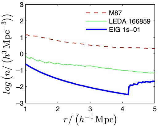
The number density, n, in a sphere of varying radius, r, around three galaxies: EIG 1s-01, LEDA 166859 – a field galaxy, M87 – cluster galaxy.
EIG 1s-01 has no neighbours closer than 4 h−1 Mpc but has 10 neighbours at a distance of 4–5 h−1 Mpc. As can be seen in Fig. 1, in the range of calculated sphere radius (1 < r < 5 h−1 Mpc) the neighbourhood density of EIG 1s-01 is about one order of magnitude lower than that of the typical field galaxy (LEDA 166859) and about two orders of magnitude lower than that of the cluster galaxy (M87). This typical example indicates that the EIGs are extreme field galaxies, significantly more isolated than the average.
Next, specific neighbourhood data of each EIG are listed. Table 8 summarizes information about the observed neighbourhood of the EIGs of subsamples EIG-1 and EIG-2 (objects that passed the isolation criterion). The distance to the nearest known neighbour, d1, obtained separately from the NED and α.40 data sets, is listed. For ALFALFA, the number of known neighbours up to a distance of 3 h−1 Mpc (neighbour count) is also listed (for NED it is zero by definition) along with the data set coverage where ‘Full’ indicates that the sphere of radius 3 h−1 Mpc around the galaxy is fully covered by the α.40 data set and ‘Partial’ indicates that only a part of this sphere is covered. The table also lists the name of the void in which the EIG is located (or the names of two adjacent voids, in case of a nameless void). The void names are as defined in the ‘Atlas of nearby large-scale structures’ of Fairall (1998).
Observed neighbourhood of EIGs (subsamples 1 and 2).
| NED | ALFALFA | ||||
|---|---|---|---|---|---|
| EIG | d1 | d1 | Neighbour | Coveragea | Void |
| name | (h−1 Mpc) | (h−1 Mpc) | counta | name | |
| 1s-01 | 4.19 | 4.32 | 0 | Partial | Canis Major |
| 1s-02 | 3.22 | 3.95 | 0 | Full | Canis Major |
| 1s-03 | 4.35 | 5.99 | 0 | Partial | Canis Major |
| 1s-04 | 3.02 | 3.01 | 0 | Full | Ursa Major–Canis Majorb |
| 1s-05 | 3.01 | 3.05 | 0 | Full | Ursa Major–Hydrab |
| 1s-06 | 3.11 | 3.11 | 0 | Partial | Ursa Major–Hydrab |
| 1s-07 | 3.27 | 5.07 | 0 | Partial | Ursa Major–Hydrab |
| 1s-08 | 4.02 | 4.18 | 0 | Partial | Leo–Hydrab |
| 1s-09 | 3.07 | 3.30 | 0 | Full | Leo–Hydrab |
| 1s-10 | 3.02 | 3.22 | 0 | Partial | Coma |
| 1s-11 | 3.91 | 4.04 | 0 | Full | Coma |
| 1s-12 | 3.28 | 3.96 | 0 | Partial | Coma |
| 1s-13 | 5.46 | 3.73 | 0 | Partial | Microscopium |
| 1s-14 | 3.45 | 3.40 | 0 | Partial | Microscopium |
| 1a-01 | 3.20 | 3.69 | 0 | Partial | Pisces |
| 1a-02 | 3.28 | 3.33 | 0 | Partial | Pisces |
| 1a-03 | 3.95 | 4.98 | 0 | Partial | Taurus |
| 1a-04 | 3.35 | 3.21 | 0 | Partial | Pisces |
| 1a-05 | 3.10 | 3.10 | 0 | Partial | Pisces |
| 1a-06 | 4.49 | 4.49 | 0 | Partial | Taurus |
| 1a-07 | 4.42 | 4.43 | 0 | Partial | Delphinus |
| 2s-01 | 3.24 | 1.07 | 2 | Full | Canis Major |
| 2s-02 | 3.61 | 0.66 | 1 | Full | Canis Major |
| 2s-04 | 3.00 | 1.90 | 2 | Full | Coma |
| 2s-05 | 3.32 | 0.94 | 3 | Partial | Microscopium |
| 2s-06 | 3.31 | 1.57 | 3 | Partial | Microscopium |
| 2s-07 | 3.43 | 2.37 | 1 | Full | Virgo–Microscopiumb |
| 2s-08 | 3.21 | 1.71 | 1 | Partial | Microscopium |
| 2a-01 | 3.11 | 1.19 | 1 | Partial | Pisces |
| 2a-02 | 3.30 | 1.63 | 4 | Partial | Pisces |
| 2a-03 | 3.47 | 1.60 | 4 | Full | Pegasus |
| 2a-04 | 3.14 | 2.74 | 1 | Partial | Pegasus |
Notes.a‘Neighbour count’ and ‘Coverage’ refer to a sphere of radius 3 h−1 Mpc around the EIG.
bA void between the two voids, whose names are listed.
Table 9 summarizes the observed neighbourhood data for subsample EIG-3 (those galaxies which fell short of passing the isolation criterion, but were still studied). In addition to the fields listed in Table 8, the table lists the neighbour counts obtained from the NED data set.
Investigation of EIG coordinates in the ‘Atlas of nearby large-scale structures’ (Fairall 1998) shows that most EIGs reside close to walls and filaments rather than in centres of voids. This may explain why there is no EIG with d1 ≥ 4.5 h−1 Mpc (as can be seen in Tables 8 and 9).
Observed neighbourhood of EIGs (subsample 3).
| NED | ALFALFA | |||||
|---|---|---|---|---|---|---|
| EIG | d1 | Neighbour | d1 | Neighbour | Coveragea | Void |
| name | (h−1 Mpc) | counta | (h−1 Mpc) | counta | name | |
| 3s-01 | 2.86 | 1 | 3.14 | 0 | Full | Ursa Major–Hydrab |
| 3s-02 | 2.29 | 1 | 1.96 | 3 | Full | Coma |
| 3s-03 | 2.87 | 1 | 0.97 | 4 | Partial | Coma |
| 3s-04 | 2.98 | 1 | 2.98 | 1 | Partial | Coma |
| 3s-05 | 2.83 | 1 | 5.12 | 0 | Full | Microscopium |
| 3s-06 | 2.44 | 4 | 3.71 | 0 | Partial | Virgo |
| 3s-07 | 2.73 | 1 | 3.82 | 0 | Partial | Microscopium |
| 3a-01 | 2.40 | 1 | 2.39 | 1 | Partial | Pegasus |
| 3a-02 | 2.37 | 1 | 2.37 | 1 | Partial | Pisces |
Notes.a‘Neighbour count’ and ‘Coverage’ refer to a sphere of radius 3 h−1 Mpc around the EIG.
bA void between the two voids, whose names are listed.
A part of the Spring sky region, in which the α.40 data set covers a 3 h−1 Mpc radius sphere around each point (|$ {8^{\rm h}} < {\alpha } < {16^{\rm h}}$|, 9° < δ < 11°, 3500 < cz < 7000 km s−1) was statistically analysed. The number density of NED galaxies in this region is 0.065 h3 Mpc−3, while the number density of ALFALFA galaxies in this region is 0.039 h3 Mpc−3. The average number of NED neighbours to a distance of 3 h−1 Mpc around each NED galaxy in the above-mentioned region was found to be 27.5 ± 0.9 (where the uncertainty is statistical and does not include the effect of uncertainties in cz, which is expected to be minor). The average number of ALFALFA neighbours to a distance of 3 h−1 Mpc around each NED galaxy in this region was found to be 14.3 ± 0.5. This is equivalent to a number density of 0.243 ± 0.008 h3 Mpc−3 NED neighbours, and 0.126 ± 0.001 h3 Mpc−3 ALFALFA neighbours, which means that the 3 h−1 Mpc neighbourhood of randomly selected NED galaxies is three to four times denser, on average, than the average density in the entire region. This result is expected, given the clustered nature of galaxy distribution in the Universe.
The ALFALFA neighbour counts (number of ALFALFA neighbours to a distance of 3 h−1 Mpc listed in Table 8) of Spring galaxies that passed the criterion using NED data (subsamples EIG-1s and EIG-2s) and had full ALFALFA coverage were also statistically analysed. Their measured distribution fits well a Poisson distribution with an expected value of |$0.7^{+0.4}_{-0.3}$| ALFALFA neighbours per EIG. Therefore, the average number density of ALFALFA neighbours within 3 h−1 Mpc from these EIGs is |$0.006^{+0.004}_{-0.003}\,h^{3}\, {Mpc}^{-3}$|. This means that, on average, the number density around EIGs (1s and 2s) of ALFALFA galaxies is only |$0.05^{+0.03}_{-0.02}$| of the number density around random NED galaxies.
2.5 Comparison to other IG samples
The ‘CIG’ (Karachentseva 1973; Karachentseva, Lebedev & Shcherbanovskij 1986) was used as the basis of the AMIGA international project (Verley et al. 2007; Fernández Lorenzo et al. 2013). It defines a galaxy as isolated if it has no neighbours with angular diameter in the range |$\frac{1}{4} a$| to 4a up to a projected angular distance of 20a, where a is the angular diameter of the tested galaxy. Hirschmann et al. (2013) estimated that a sample based on the AMIGA (Verley et al. 2007) 2D criterion will include a fraction of ∼18 per cent false positives due to projection effects. For an angular diameter a = 20 kpc, for example, the Karachentseva (1973) criterion corresponds to having no neighbours with angular diameters in the range 5–80 kpc up to a distance of 0.4 Mpc. Compared to this, the 4.26 Mpc distance criterion used in this work tests for a significantly higher level of isolation.
The same CIG 2D criterion was used for two other catalogues of IGs. The ‘2MIG’ catalogue was created by Karachentseva et al. (2010) from the ‘Two Micron All-Sky Survey’ (2MASS; Skrutskie et al. 2006) data using the selection criterion from CIG. The ‘LOG’ catalogue (Karachentsev et al. 2011) was produced by combining a 3D redshift-space-based criterion with the CIG 2D criterion. The LOG sample includes 520 IGs selected from a region defined by galactic latitudes |b| > 15° and with radial velocities smaller than 3500 km s−1 relative to the centroid of the Local Group. Their 3D criterion confirmed that the LOG sample galaxies are not part of gravitationally bound groups that would survive the Hubble expansion. It assumed that 2MASS K-band luminosities are proportional to the total mass of galaxies. Their K-band luminosity-to-mass relation was tuned so that 10 per cent of the galaxies would pass the criterion (i.e. would not be identified as part of a group).
The VGS (Kreckel et al. 2012) applied a redshift space criterion, very different from that used in this work. Kreckel et al. (2012) used SDSS DR7 data to reconstruct the density field from the spatial galaxy distribution (in the redshift range 900 < cz < 9000 km s−1). Void regions were then identified in this density field using a ‘watershed finder algorithm’ that does not assume a particular void size or shape. 60 VGS sample galaxies were then selected to be as close as possible to the centres of these voids.
We tested the observed neighbourhoods of all galaxies of these four catalogues that are within the EIG search regions (defined in Table 1). The process and data sets used were identical to those used for the EIG selection. For each of the four catalogues, the probabilities of galaxies qualifying for each of the EIG subsamples (EIG-1, EIG-2 and EIG-3) are listed in Table 10.
Other IG catalogues – probability of qualification as EIGs.
| Fraction [number]a qualifying as | ||||
|---|---|---|---|---|
| Catalogue | EIG-1 | EIG-2 | EIG-3 | None |
| AMIGA | (|$0^{+0.08}_{-0}$|) [0] | (|$0^{+0.08}_{-0}$|) [0] | (|$0.07^{+0.12}_{-0.05}$|) [3] | (|$0.93^{+0.05}_{-0.12}$|) [40] |
| 2MIG | (|$0^{+0.07}_{-0}$|) [0] | (|$0^{+0.07}_{-0}$|) [0] | (|$0.04^{+0.10}_{-0.03}$|) [2] | (|$0.96^{+0.03}_{-0.10}$|) [47] |
| LOG | (|$0^{+0.26}_{-0}$|) [0] | (|$0^{+0.26}_{-0}$|) [0] | (|$0.09^{+0.29}_{-0.07}$|) [1] | (|$0.91^{+0.07}_{-0.29}$|) [10] |
| VGS | (|$0.33^{+0.37}_{-0.24}$|) [2] | (|$0^{+0.39}_{-0}$|) [0] | (|$0.50^{+0.31}_{-0.31}$|) [3] | (|$0.17^{+0.40}_{-0.14}$|) [1] |
Notes.aIn square brackets are the numbers of tested IGs of each catalogue that qualify for each EIG subsample (or, under ‘None’, that do not qualify for any subsample).
As evident from the table, only a small fraction of the AMIGA, 2MIG and LOG catalogues may qualify as EIG-3 galaxies (galaxies for which the distance to the closest neighbour in NED's data is 2–3 h−1 Mpc). None of the AMIGA, 2MIG and LOG galaxies (within the regions defined in Table 1) fitted the EIG-1 or EIG-2 criterion, and none are part of the sample studied here (the EIG-3 subsample is not complete, i.e. does not include all galaxies that pass its criterion). However, there is one 2MIG galaxy (outside the regions defined in Table 1), 2MIG 302, which is an EIG-1 galaxy (EIG 1a-04). It is not included in the statistics of Table 10 since it lies outside the search region (as mentioned in Section 2.3).
Only six galaxies from the VGS catalogue are within the search regions of the EIG sample. Three of these pass the criterion for the EIG-3 subsample, but are not part of it. One galaxy, VGS_52, is an EIG-1 galaxy (EIG 1s-13). Another galaxy, VGS_23, marginally qualifies as an EIG-1 galaxy and was not included in the sample studied here. The sixth VGS galaxy does not qualify for any of the EIG subsamples.
Distances to the closest neighbour listed in either the NED or α.40 data sets, d1, were measured for all AMIGA, 2MIG, LOG and VGS galaxies in the EIG search regions. Based on these, the probability distribution function (PDF) of d1 was calculated for each catalogue (Fig. 2). For comparison, Fig. 3 shows the PDF of d1 for each of the EIG subsamples and for the EIG-1 and EIG-2 subsamples together (all galaxies that passed the isolation criterion using the NED data set).
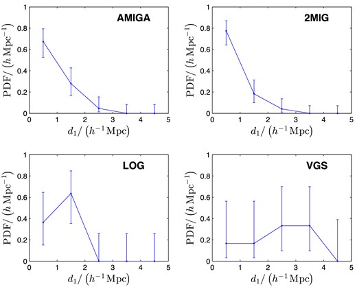
PDF of the distance to the closest neighbour, d1, for the AMIGA, 2MIG, LOG and VGS IG catalogues.
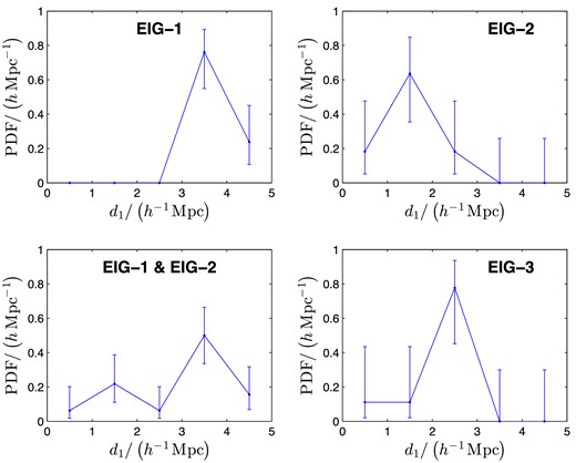
PDF of the distance to the closest neighbour, d1, for each subsample: ‘EIG-1’, ‘EIG-2’ and ‘EIG-3’, and for the ‘EIG-1 & EIG-2’ subsamples together.
It is evident from these figures that the d1 of AMIGA, 2MIG and LOG galaxies is typically significantly lower than the d1 of EIG galaxies. The average d1 of the tested galaxies was 0.83 h−1 Mpc for AMIGA, 0.74 h−1 Mpc for 2MIG and 1.19 h−1 Mpc for LOG, compared to 3.54 h−1 Mpc for the EIG-1 subsample, 1.58 h−1 Mpc for the EIG-2 subsample and 2.39 h−1 Mpc for the EIG-3 subsample. The average d1 of the EIG-1 and EIG-2 subsamples together is 2.86 h−1 Mpc. The PDF for the VGS catalogue reaches higher d1 values compared to the other three catalogues. The average d1 measured for the six tested VGS galaxies is 2.39 h−1 Mpc.
We conclude that the EIG sample studied here is indeed extreme in its measurable isolation. The use of H i redshifts from ALFALFA proved to be a key factor in identifying the most extremely isolated subsample (EIG-1).
3 PROPERTIES ESTIMATED USING COSMOLOGICAL SIMULATIONS
This section describes the analysis of cosmological simulations we performed to estimate properties of the EIG-1 and EIG-2 subsamples. Two cosmological simulations were used for this analysis (described in Section 3.1) using which mock EIG samples were created (Sections 3.2 through 3.4). By comparing these with random mock samples, properties of the EIGs were statistically estimated.
In Section 3.5, properties of the DM haloes are analysed. These include the halo's mass and whether it is dominant in its immediate neighbourhood. In Section 3.6, mass accretion histories (MAHs) are analysed. Next, the neighbourhoods of the EIGs are analysed in terms of galaxy number density (Section 3.7), halo number density (Section 3.8) and DM mass density (Section 3.9). Finally, the tidal acceleration exerted on EIGs by their neighbouring DM haloes is analysed (Section 3.10).
As discussed in Section 2.1, the neighbourhood measurement is limited by two factors: incompleteness of the redshift data (i.e. redshift data are not available for a significant fraction of the galaxies) and peculiar velocities that introduce an error in the distance measurement. Due to these, the actual neighbourhood of an individual EIG may differ significantly from what it seems to be from the data in Tables 8 and 9, or from the number density functions, such as shown in Fig. 1.
However, as a sample, rather than individually, the probabilities of neighbourhood properties can be derived using cosmological simulations. These simulations describe mock universes with detailed information on DM haloes and galaxies that reside in them. By applying the same search process used previously to select the EIG sample on these mock universes, mock EIG samples were created for which the simulated properties were calculated. The distribution of these properties in the mock EIG samples serves as an estimate of the PDFs of these properties in the real EIG sample.
The derivation process of the PDFs included the following steps.
Defining points of view and sky regions in the mock universes, simulating the observer and the sky region in which the mock EIGs are searched for.
Estimating ‘completeness’ functions of the NED data, which define for each given observable magnitude, the fraction of galaxies in the search region for which a redshift measurement was available in the NED data set. The ‘completeness’ functions of the Spring and Autumn regions were measured separately, since they are significantly different (the Spring region is fully covered by SDSS, while the Autumn region is not). The ‘completeness’ functions were estimated separately for each of the simulations.
Creating ‘mock observable’ data sets, each including all coordinates and simulation IDs of galaxies, randomly selected using the ‘completeness’ function. These ‘mock observable’ data sets imitate the data that would have been available from NED, had the ‘mock universes’ been the real Universe. For each simulation, point of view and sky region, several such ‘mock observable’ data sets were created.
Creating ‘mock EIG samples’ by applying the sample selection process (described in Section 2.2) on the ‘mock observable’ data sets. These are divided into ‘Spring mock EIG samples’, which simulate subsamples EIG-1s and EIG-2s (together), and ‘Autumn mock EIG samples’, which simulate subsamples EIG-1a and EIG-2a (together).
Creating ‘mock random samples’ by randomly selecting a thousand galaxies from each ‘mock observable’ data set. These ‘mock random samples’ are used as reference to the ‘mock EIG samples’, when evaluating their properties’ PDFs.
‘Measuring’ simulated properties of ‘mock EIG samples’ and ‘mock random samples’ galaxies, and creating histograms that estimate the PDFs of these properties in the real Universe EIG sample and in real Universe random galaxies.
Note that at the time this analysis was performed no cosmological simulation claimed to estimate the H i content of galaxies with reasonable accuracy.5 Therefore, the ‘completeness’ functions were defined for the luminous content only, and not for H i content (21 cm fluxes). The estimated PDFs discussed below, therefore, relate more closely to the EIG-1 and EIG-2 subsamples together (all galaxies that passed the isolation criterion using the NED data set), rather than to each subsample separately.
As already shown in Section 2.3, the use of ALFALFA significantly improves the quality of the sample. Therefore, the isolation properties of the EIG-1 subsamples are expected to exhibit significantly more isolated-like PDFs compared to the PDFs estimated here (for EIG-1 and EIG-2 together).
3.1 Simulations
The following two cosmological simulations were used independently for the EIG history and neighbourhood analysis.
3.1.1 Millennium II-SW7 (Mill2)
The Millennium II-SW7 simulation (Mill2; Guo et al. 2013) made publicly available by the Virgo Consortium (Lemson et al. 2006) is an updated version of the Millennium-II simulation (Boylan-Kolchin et al. 2009) in which the structure growth in a ΛCDM universe was scaled to parameters consistent with WMAP7 (Bennett et al. 2011). The properties of galaxies were simulated using the semi-analytical model (SAM) described in Guo et al. (2013).
Mill2 simulates a cube with edge length of 104.311 h−1 Mpc, and uses 21603 particles of mass Mp = 8.5024 × 10⁶ h− 1 M⊙ each. It uses the following cosmological parameters: h = 0.704, ΩΛ = 0.728 (density parameter for dark energy), Ωm = 0.272 (density parameter for matter), Ωb = 0.045 (density parameter for baryonic matter), ns = 0.961 (normalization of the power spectrum) and σ8 = 0.807 (amplitude of mass density fluctuation in 8 h−1 Mpc sphere at z = 0).
Two types of halo classifications are defined in Mill2.
Friends-of-Friends (FOF) groups – defined with b = 0.2 (Boylan-Kolchin et al. 2009).6
(Sub)Haloes – the decomposition of the FOF groups into gravitationally bound haloes.
For each subhalo, a merger tree can be extracted from the simulation, which includes data on all its progenitors since the beginning of the simulated time [lookback time (LBT) of 13.75 Gyr]. The merger tree and physical properties of each progenitor subhalo are the inputs of the SAM. The halo data set used for the analysis described in this work was limited by halo mass Mhalo ≥ 109 h− 1 M⊙.
As described above at the beginning of Section 3, the analysis required choosing a point of view (simulating the our Galaxy) and its tested sky region. Simulated EIGs were then searched for in this sky region, using data in the redshift range 1600–7400 km s−1 (same as used for the search in the NED data set). Mill2's simulated box is too small to allow a 4π sr coverage to this range. To simplify the search algorithm (avoiding the use of the simulation's periodic boundary conditions), the point of view was chosen to be close to the simulation's point of origin (one of the corners of the simulated cube) at |$\boldsymbol {r} = \left(20.0\,, 20.0\,, 20.0\right)\,h^{-1}\,{Mpc}$|, and the tested sky region was chosen to be the (+,+,+) octant. The 20.0 h−1 Mpc distance in each axis from the cube's corner was chosen to allow a simplified search around the edges of the search region.
3.1.2 Box160
The Box160 simulation is a constrained simulation of the local Universe, based on the ΛCDM third-year WMAP (WMAP3; Spergel et al. 2007) which simulates a cube with 160 h−1 Mpc edges (Gottlöber & Klypin 2008; Forero-Romero et al. 2009). It is part of the Constrained Local UniversE Simulations (CLUES) project (Gottlöber, Hoffman & Yepes 2010). Its DM distribution emulates large structures in the local Universe (Virgo, Coma, Local Supercluster, etc.). Box160 uses 10243 DM particles each of mass Mp = 2.54 × 10⁸h− 1 M⊙, and the following cosmological parameters: h = 0.73, ΩΛ = 0.76, Ωm = 0.24, ns = 0.96 and σ8 = 0.76.
Unlike Mill2, in Box160 the FOF haloes are not divided into gravitationally bound subhaloes. Instead, the FOF haloes are directly populated with simulated galaxies (a single FOF halo may contain more than one galaxy). The algorithm applied for this is a conditional luminosity function algorithm similar to that of van den Bosch et al. (2007) but without distinction between central and satellite galaxies (which may somewhat alter the probability that close central–satellite pairs will be detected as non-isolated). The faintest simulated galaxy luminosity is 3.305 × 10⁷h− 2 L⊙, corresponding to Mg = −14.44. The Box160 data set used here contains haloes of mass 1.814 × 10¹⁰ h− 1 M⊙ and above.
For the analysis of Box160, two points of view were used from which the neighbourhood resembles that of the our Galaxy (Gottloeber & Hoffman, private communication). These points, around which the entire 4π sr sky was tested, are defined by their location, |$\boldsymbol {r}$|, and by their peculiar velocity (relative to the comoving coordinates), |$\boldsymbol {v}_{{\rm p}}$|, as follows:
LG1 : |$\boldsymbol {r} = \left(79.3241 \,,\ 56.0739 \,,\ 84.7330 \right) \,h^{-1}\,{Mpc},$|
|$\boldsymbol {v}_{{\rm p}} = \left(28.7 \,,\ 427.8 \,,\, -340.1 \right) \,{\rm km\,s}^{-1}$|
LG2 : |$\boldsymbol {r} = \left(74.9237 \,,\ 63.8382 \,,\ 80.4162 \right) \,h^{-1}\,{Mpc},$|
|$\boldsymbol {v}_{{\rm p}} = \left(-172.4 \,,\ 511.2 \,,\, -349.5 \right) \,{\rm km\,s}^{-1}$|.
Compared to the Mill2 simulation, Box160 is inferior in mass resolution and in the fact that it uses older cosmological parameters. However, since it simulates the local Universe, it enables analysing the isolation criterion from a point of view resembling ours in the real Universe. This, along with the differences in halo definition and method of populating the haloes with galaxies, serves as a tool for estimating the sensitivity of the results to these important simulation details.
3.2 The completeness functions
In order to estimate the completeness function (described at the beginning of Section 3), the number density of galaxies per magnitude interval, ngal/Δm, was derived both for the simulations and for the NED data sets. For the simulations, ngal/Δm was calculated for the same redshift range as that of the NED data sets, i.e. 1600–7400 km s−1.
Fig. 4 shows the galaxy number density per magnitude interval, ngal/Δm, for the Mill2 simulation, Box160 simulation, NED's Spring region and NED's Autumn region. For Box160, ngal/Δm was measured from both points of view (LG1 and LG2). The results for LG1 and LG2 were very similar (less than 9 × 10⁻⁴ h3 Mpc−3 mag−1 apart at any point). The curve displayed in the figure for Box160 is the average between them.
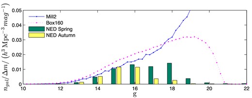
The number density of galaxies per magnitude interval, ngal/Δm, for the Mill2 simulation, Box160 simulation (average between LG1 and LG2), NED's Spring region and NED's Autumn region (redshift range: 1600 ≤ cz ≤ 7400 km s−1).
As Fig. 4 shows, ngal/Δm of Mill2 and Box160 are somewhat different for g < 18. The Box160 curve peaks at g ≅ 19, while the Mill2 curve continues to rise and peaks only at g = 28.7 with a value of ∼0.7 h3 Mpc−3 mag−1. These differences are believed to be mainly due to the different method by which these simulations populate haloes with galaxies. The SAM used by Mill2 can create extremely low luminosity galaxies, effectively extrapolating far beyond the accurately measured range of the galaxy luminosity function (LF). Box160, on the other hand, populates haloes by imitating the measured LF, and therefore cannot extrapolate beyond the LF established range.
It is also evident from Fig. 4 that ngal/Δm of the NED Spring region differs significantly from that of the NED Autumn region. The fact that ngal/Δm of the Autumn region is cut off at brighter magnitudes compared to the Spring region hints that this is due to completeness differences, where the Spring region is complete to fainter magnitudes. This is probably because the Spring region is fully covered spectroscopically by SDSS, while the Autumn region is not. However, the difference in ngal/Δm may also be attributed to a real difference in the large-scale structure of these two regions; the density of faint galaxies in the Autumn region may really be lower in comparison to the Spring region. The analysis of the simulations assumes an average composition of the large-scale structures. Any deviation from an average composition (in the Spring or Autumn regions) affects the accuracy of the completeness function estimation, which propagates to the accuracy of the calculated PDFs. Evidence for such a deviation is discussed in Section 3.4.
gmax is the cutoff g magnitude above which no galaxy is observed and
fracobs is the fraction of galaxies observed below the cutoff magnitude.
This model emulates typical spectroscopic surveys in which the redshifts of galaxies dimmer than a limiting magnitude (gmax) are not measured at all, while not all of the brighter galaxies are measured. This is obviously not an accurate model for data sets such as NED, which include a combination of many spectroscopic surveys.
One alternative to this simplified completeness model is to apply a completeness correction for each magnitude bin separately. This would trace more tightly the ngal/Δm of NED's Spring and Autumn regions compared to the simplified model used here. However, this might cause inaccuracies when overdensities or underdensities in certain magnitude bins (due to, for example, variation from the average composition of the large-scale structures) will be falsely translated to overestimates or underestimates in the completeness function.
The variables fracobs and gmax were calculated to provide simultaneous fits to the following two parameters:
the galaxy number density (ngal/Δm integrated over all magnitudes) and
ngal/Δm integrated over the decreasing slope (g ≥ 17.5 for the Spring region and g ≥ 15.5 for the Autumn).
This ensures that the overall number density, as well as the number density of the dimmer galaxies, is well simulated in the mock observable data sets.
The best-fitting parameters of the completeness function are listed in Table 11. As can be seen, gmax is significantly larger for the Spring region, while fracobs is somewhat larger for the Autumn region. There are large differences between the parameters of the Mill2 simulation and those of the Box160 simulation. These are the result of the differences in the ngal/Δm functions, discussed above.
The completeness functions’ fitted parameters.
| Region | Simulation | fracobs | gmax | |
|---|---|---|---|---|
| Spring | Mill2 | 0.714 | 18.4 | |
| Box160 | 0.574 | 18.7 | ||
| Autumn | Mill2 | 0.863 | 16.8 | |
| Box160 | 0.635 | 16.9 |
| Region | Simulation | fracobs | gmax | |
|---|---|---|---|---|
| Spring | Mill2 | 0.714 | 18.4 | |
| Box160 | 0.574 | 18.7 | ||
| Autumn | Mill2 | 0.863 | 16.8 | |
| Box160 | 0.635 | 16.9 |
3.3 The mock observable data sets
The ‘mock observable’ data sets were created using the procedure described at the beginning of Section 3 and using the completeness functions described in Section 3.2. For the Mill2 simulations, five mock observable data sets were created for the Spring region, and five for the Autumn region. For the Box160 simulation, three mock observable data sets were created for each point of view (LG1 and LG2) and region, for a total of six mock observable data sets for the Spring region and six for the Autumn region.
For each mock observable data set, the ngal/Δm function was calculated. The functions were averaged for each of the four simulation and sky region pairs. These average functions are shown in Fig. 5, along with the NED ngal/Δm to which they were fitted. The vertical error bars in the figure show the standard deviation of the averaged functions.
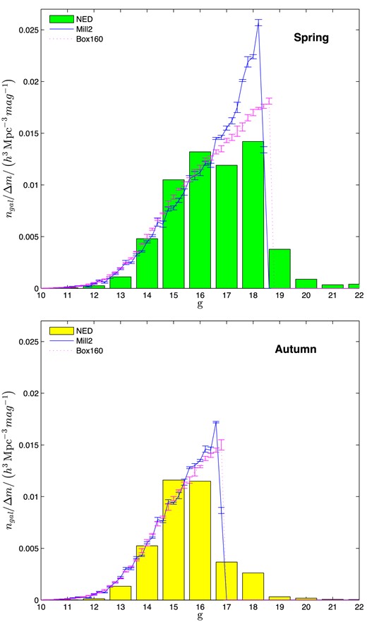
A comparison of ngal/Δm of the Mill2 mock observable data sets, Box160 mock observable data sets and NED (in the redshift range: 1600 ≤ cz ≤ 7400 km s−1).
As Fig. 5 shows, the mock observable data sets trace approximately the real NED ngal/Δm function. In the range g < 16, the fit is reasonably well. In the ranges 16 < g < 18 for the Spring region and 16 < g < 17 for the Autumn region, there is an excess of simulated galaxies. Due to the method by which the completeness function was fitted, this excess averages with the deficiency above the cutoff magnitude, gmax, in which by definition there are no simulated galaxies so that the overall number densities of galaxies in the simulations are the same as in NED.
3.4 The mock EIG samples
‘Mock EIG samples’ were created by applying the search criterion described in Section 2.1 to each mock observable data set. The fraction of galaxies with known redshifts that passes the isolation criterion, fracEIG, and the number density of the EIGs, nEIG, were calculated for each mock EIG sample and for the real NED data. Table 12 presents the results. For each simulation and sky region, the average values are shown with standard-deviation-based (1σ) uncertainties. The table also lists the number of mock random galaxies, Nrandom, and EIGs, NEIG, that were analysed.
EIG abundance.
| Region | Data set | Nrandom | NEIG | fracEIG (per cent) | nEIG(h3 Mpc−3) |
|---|---|---|---|---|---|
| Spring | NED | – | 21 | 0.62 ± 0.14 | (3.9 ± 0.8) × 10−4 |
| Mill2 | 5000 | 522 | 0.97 ± 0.07 | (5.0 ± 0.4) × 10−4 | |
| Box160 | 6000 | 4952 | 0.90 ± 0.03 | (4.91 ± 0.07) × 10−4 | |
| Autumn | NED | – | 10 | 2.6 ± 0.8 | (11 ± 3) × 10−4 |
| Mill2 | 4000 | 625 | 1.96 ± 0.05 | (6.0 ± 0.2) × 10−4 | |
| Box160 | 6000 | 6449 | 1.99 ± 0.09 | (6.40 ± 0.15) × 10−4 |
As Table 12 shows, the simulations reproduce the real EIG abundance to within ∼2σ in both measured parameters. The abundance of Autumn EIGs is significantly larger than the abundance of Spring EIGs. The Autumn-to-Spring abundance ratio is larger in the real NED data (4 ± 2 in fracEIG and 3 ± 1 in nEIG) compared to the simulations (a factor of 2.17 ± 0.08 in fracEIG and 1.26 ± 0.03 in nEIG). This may be attributed to a real difference between the large-scale structure of the Autumn and Spring regions, which is not accounted for in the simulations.
3.5 Halo properties
EIGs are expected to reside in (sub)haloes that are the dominant ones in their FOF group, i.e. haloes that do not have neighbours of comparable mass within the FOF group. The Mill2 simulation was analysed to find out which of the galaxies reside in such dominant subhaloes, where a dominant subhalo is defined here as one lacking subhalo neighbours in its FOF halo with mass ≥25 per cent of its own. The fraction of galaxies residing in dominant subhaloes, fracdominant, was calculated for the mock EIG samples and for the mock random samples in both sky regions. The results are presented in Table 13.
Fraction dominant in FOF halo.
| Region | Sample | fracdominant |
| Spring | EIG | 0.94 ± 0.02 |
| Random | 0.54 ± 0.01 | |
| Autumn | EIG | 0.91 ± 0.01 |
| Random | 0.58 ± 0.02 |
| Region | Sample | fracdominant |
| Spring | EIG | 0.94 ± 0.02 |
| Random | 0.54 ± 0.01 | |
| Autumn | EIG | 0.91 ± 0.01 |
| Random | 0.58 ± 0.02 |
Table 13 shows that the fraction of EIGs that are dominant in their FOF haloes is significantly larger than the overall fraction of dominant galaxies (‘measured’ in the random samples). This dominant fraction is slightly larger for Spring EIGs than for Autumn EIGs, probably due to the higher completeness of the Spring data. The Autumn overall dominant fraction is slightly larger than the Spring one, probably due to the fact that the Autumn mock observable data sets contain fewer dim galaxies, which are more abundant in satellite subhaloes.
The PDFs of the galaxies’ subhalo mass, Mhalo, were ‘measured’ in Mill2 and are shown in Fig. 6. The figure compares the Mhalo PDF of EIGs with that of randomly selected galaxies, for both the Spring (left-hand panel) and Autumn (right-hand panel) regions. Fig. 6 shows that the Mhalo of the EIGs is less scattered than that of the random population. This is more pronounced in the Spring region, where the standard deviation of log[Mhalo/(h− 1 M⊙)] is ∼0.3 for the EIGs, compared to ∼0.8 for the random sample (for the Autumn region it is ∼0.4 for the EIGs, compared to ∼0.7 for the random sample).
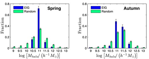
Distribution of subhalo mass, Mhalo, in Mill2 mock data sets (EIG and random).
Interestingly, there's no significant difference in the average log[Mhalo/(h− 1 M⊙)] between the EIG and the random samples. In the Spring region, it is 11.0 (EIGs) versus 10.9 (random). In the Autumn region, it is 11.3 (EIGs) versus 11.2 (random). The difference between the two regions can be explained by the Spring region completeness function that reaches fainter magnitudes. The fainter galaxies included in the Spring data set typically reside in lower mass haloes.
The Mill2 simulation, therefore, predicts that IGs tend to reside in haloes of average mass, rather than in low- or high-mass haloes. The fraction of EIGs in haloes of Mhalo > 1012 h− 1 M⊙ or Mhalo < 1010 h− 1 M⊙ is significantly smaller than this fraction in a random population. The low abundance of EIGs with Mhalo > 1012 h− 1 M⊙ may be attributed to the low mass density in the isolated regions where EIGs reside, which possibly does not allow them to accrete so much mass.
One may speculate that for Mhalo < 1010 h− 1 M⊙, this could be the result of a selection effect, if EIGs in low-mass haloes had significantly lower luminosities compared to random galaxies of the same halo mass. In such case, the EIGs of low halo mass would not have been detectable due to their extremely low luminosities. However, this does not seem to be the case. A comparison between the absolute magnitudes of the EIGs and random galaxies of the same mass bins shows that in the central bins (1010.5–1012 h− 1 M⊙) the average difference is much smaller than its standard deviation, and would not explain this phenomenon. For the lower mass bins, the few EIGs found in Mill2 even show a tendency to be brighter than the random galaxies.
The explanation for the low abundance of EIGs with Mhalo < 1010 h− 1 M⊙ seems to be related to the low rate of ‘major events’ they undergo (major mergers or significant mass-loss events), as defined and analysed in Section 3.6. This is evident from a comparison between Figs 6 and 7, which shows the Mhalo PDF of subhaloes that did not experience a ‘major event’ in their past. In the range Mhalo ≤ 1010 h− 1 M⊙, the PDF of random galaxies that did not experience a ‘major event’ is very low and similar to that of the EIGs. Therefore, ‘major events’ seem to be the main mechanism creating low-mass subhaloes (Mhalo < 1010 h− 1 M⊙) that host galaxies of Mg ≲ −14 (the magnitude range included in the Spring mock observable data set).
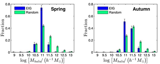
Distribution of subhalo mass, Mhalo, in Mill2 mock data sets (EIG and random) of haloes that did not experience a ‘major event’ in their past.
The PDFs of the galaxies’ FOF halo mass, MFOF, were ‘measured’ in Box160 and are shown in Fig. 8. The figure compares the MFOF PDF of EIGs with that of the randomly selected galaxies for both the Spring (left-hand panel) and Autumn (right-hand panel). Fig. 8 shows that the MFOF PDF includes higher masses, compared to the PDF of the subhaloes (Fig. 6). This is expected, since each FOF halo may contain many gravitationally bound subhaloes. As in the case of subhaloes, the EIGs’ MFOF is less scattered than that of the random samples. The standard deviation of log[MFOF/(h− 1 M⊙)] is ∼0.3 for the EIGs of the Spring region, compared to ∼1.0 for the random sample. For the Autumn region, it is ∼0.4 for the EIGs, compared to ∼1.0 for the random sample.
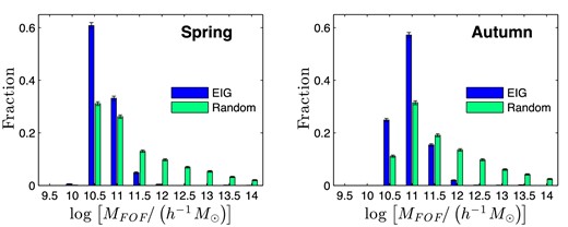
Distribution of FOF halo mass, MFOF, in the Box160 mock data sets (EIG and random).
The average log[MFOF/(h− 1 M⊙)] of EIGs is smaller than that of random galaxies. In the Spring region, it is 10.8 (EIGs) versus 11.5 (random), whereas in the Autumn region it is 11.1 (EIGs) versus 11.8 (random). This difference may be explained by the EIGs’ subhaloes being the dominant ones in their FOF haloes, as shown above. Therefore, their log[MFOF/(h− 1 M⊙)] may not be significantly larger than their log[Mhalo/(h− 1 M⊙)]. On the other hand, FOF haloes of a significant fraction of the random galaxies contain many subhaloes, which significantly increases their log[MFOF/(h− 1 M⊙)]. Similarly to the case of the subhaloes, MFOF is somewhat larger in the Autumn region, compared to the Spring region.
3.6 History of the halo
The merger trees of the haloes were analysed in the Mill2 simulation to obtain information about their MAHs and about ‘major events’ in their past. Major events are defined here as either major mergers having progenitors with at least 20 per cent of the mass of the merged halo or major mass-loss events in which a halo lost at least 10 per cent of its mass between successive simulation snapshots. Major events were counted only for the main branches of the merger trees, i.e. major events of a satellite before it merged with a halo were disregarded.
Fig. 9 shows the PDF of the number of major events a galaxy's subhalo went through in the past ∼3 Gyr (top panels) and ∼10 Gyr (bottom panels). The actual times (3.16 and 9.97 Gyr) are the closest simulation snapshots. As in previous figures, the left-hand panels show the Spring region PDFs, and the right-hand panels show the Autumn PDFs.
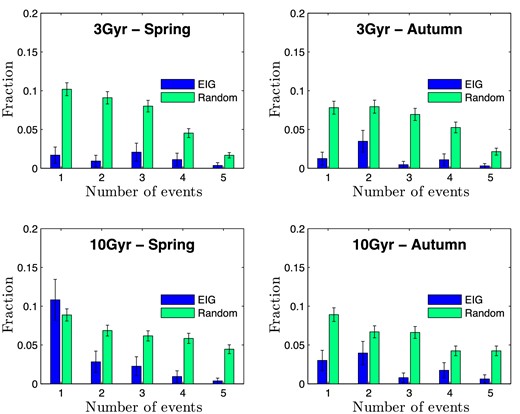
The PDF of the number of major events in the last ∼3 Gyr and ∼10 Gyr for EIGs and random galaxies.
The probability that an EIG experienced a ‘major event’ in the last 3 Gyr is only (5 ± 2) per cent for both the Spring region and the Autumn region. This, compared to (34 ± 1) per cent for a random sample galaxy in the Spring region and (31 ± 1) per cent for a random sample galaxy in the Autumn region. The small fraction of EIGs that did experience a ‘major event’ in the last 3 Gyr is the result of both the fraction of galaxies misidentified as EIGs while in fact having unobserved close neighbours and the possibility of a complete merger of two galaxies that left no neighbours.
Fig. 10 shows the PDF of the time since the last major event a galaxy's halo experienced. It appears that the PDF of the EIGs is rather similar to that of the random galaxies, except for the last 3 Gyr. In the last ∼2 Gyr, the PDF is significantly higher for the random galaxies, and is increasing as the LBT decreases. More than half of the random galaxies that experienced a major event in the last 3 Gyr had it in the last 1 Gyr.
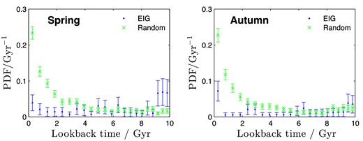
The PDF of the last major event's LBT (for EIGs and random).
The MAH of the haloes that did not experience a major event in the last 10 Gyr was analysed. The results are shown in Figs 11 and 12. In both figures, the MAH is measured as the fraction of the current halo mass which the halo accumulated at a particular LBT, MLBT/Mhalo. Fig. 11 shows the PDF of this fraction at LBT = 3 Gyr and indicates that the PDFs of EIGs and random galaxies are quite similar.

PDF of the fraction of halo mass, accreted by 3 Gyr LBT (for EIGs and random).
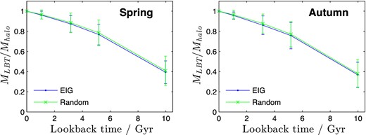
Fraction of halo mass, already accreted, as a function of the LBT (for EIGs and random galaxies that did not experience major events in the last 10 Gyr). The bars indicate the standard deviation of this fraction in the sample (rather than the measurement uncertainties).
Fig. 12 shows the average and standard deviation (indicated by bars) of MLBT/Mhalo of haloes that did not experience major events in the last 10 Gyr. Again, it is evident that the MAHs of the EIGs are very similar to those of the random galaxies, and that there is no significant difference between the Spring and the Autumn samples.
These results indicate that mass accretion (relative to the current halo mass, Mhalo) is affected by the halo's environment, mainly through strong interactions with its neighbours. As long as the halo does not experience major events, its MAH does not depend significantly on its environment.
3.7 Neighbourhood galaxies
The number density of neighbouring galaxies, ngal, around EIGs and around the random galaxies was analysed in both Box160 and Mill2. Fig. 13 shows the results for spheres of radius 3 h−1 Mpc around the galaxies and for neighbour galaxies brighter than Mg = −15. Each panel compares the ngal PDF of EIGs to that of the random galaxies. The left-hand panels show results for Spring and the right-hand panels for Autumn. The upper panels were calculated from Mill2 data and the lower ones from Box160 data.
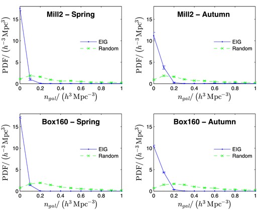
PDF of the number density of neighbouring galaxies, ngal, with Mg < −15 in a 3 h−1 Mpc radius sphere around the EIGs or random galaxies.
It is evident that the EIGs are located in significantly underdense environments compared to the general population (the random samples). It is also evident that the Spring EIGs tend to reside in lower density regions, compared to the Autumn EIGs.
The results calculated from Mill2 and Box160 agree quite well, although the difference between the Mill2 and Box160 PDF points is somewhat larger than the calculated 95 per cent (2σ) confidence level errors shown in the figure.
The fraction of Spring EIGs residing in environments with ngal < 0.1 h3 Mpc−3 is 0.98 ± 0.01 (for Mg < −15 neighbours in a 3 h−1 Mpc radius sphere). The fraction of Autumn EIGs in such environments is 0.87 ± 0.01. This, versus 0.11–0.15 of the random galaxies that reside in such ngal < 0.1 h3 Mpc−3 environments. The fraction of Spring EIGs that reside in much denser environments, with ngal > 0.5 h3 Mpc−3, is 0.02 ± 0.01 (Mill2) or 0.002 ± 0.001 (Box160). For Autumn EIGs, the fraction is 0.04 ± 0.02 (Mill2) or 0.004 ± 0.001 (Box160). This, versus 0.32–0.40 for the random galaxies. The ‘tail’ of the PDF of the random galaxies continues far beyond 1 h3 Mpc−3. In fact, a significant fraction, 0.21–0.22 (Mill2) or 0.13 (Box160), of the random galaxies reside in ngal > 1.0 h3 Mpc−3 environments, as could be expected given the clustering of galaxies.
The average number density of neighbouring galaxies, |$\overline{n_{{\rm gal}}}$|, was also analysed. Fig. 14 shows |$\overline{n_{{\rm gal}}}$| as a function of the limiting absolute magnitude, Mg,max, of the neighbouring galaxies counted in a 3 h−1 Mpc radius sphere. Fig. 15 shows |$\overline{n_{{\rm gal}}}$| as a function of the sphere radius, r, for Mg,max = −15. Both figures show that |$\overline{n_{{\rm gal}}}$| of the Spring EIGs is about one order of magnitude smaller than that of random samples in the magnitude limit range −21 < Mg,max < −15 (Fig. 14) and in the sphere radius range 2 < r < 5 h−1 Mpc (Fig. 15). For the Autumn region, |$\overline{n_{{\rm gal}}}$| of the EIGs is four to eight times smaller than that of the random samples in these ranges. The dependence of the EIGs’ |$\overline{n_{{\rm gal}}}$| on the limiting magnitude, Mg,max, and on the sphere radius, r, is quite similar to that of random galaxies.
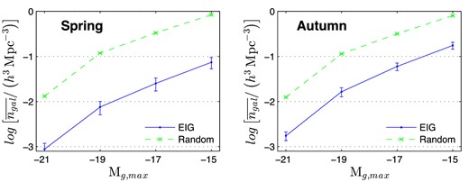
Average number density of neighbouring galaxies, |$\overline{n_{{\rm gal}}}$|, in a 3 h−1 Mpc radius sphere around the EIGs or random galaxies, as a function of limiting absolute magnitude, Mg,max (calculated using Mill2).
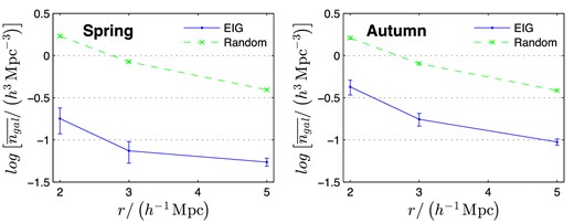
Average number density of neighbouring galaxies, |$\overline{n_{{\rm gal}}}$|, with Mg < −15 as a function of the sphere's radius around the EIGs or random galaxies, r, in which the density is averaged (calculated using Mill2).
3.8 Neighbourhood haloes
The number density of neighbouring haloes, nhalo, around EIGs and around the random galaxies was analysed for both the FOF haloes of Box160 and the gravitationally bound subhaloes of Mill2. The results are similar to those of the ngal analysis. Fig. 16 shows the results for neighbouring haloes with mass Mhalo > 1011 h− 1 M⊙ in spheres of radius 3 h−1 Mpc around the galaxies.
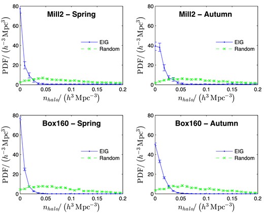
PDF of the number density of neighbouring haloes, nhalo, with Mhalo > 1011 h− 1 M⊙ in a 3 h−1 Mpc radius sphere around the EIGs or random galaxies.
As in the case of ngal, Fig. 16 shows that EIGs populate environments significantly less dense than those of the general population (random samples), and that Spring EIGs tend to reside in lower density regions compared to the Autumn EIGs. The results calculated from Mill2 and Box160 agree. The difference between the Mill2 and Box160 PDFs is mostly within the plotted 95 per cent confidence level errors. The fraction of Spring EIGs that reside in environments with nhalo < 0.03 h3 Mpc−3 is 0.98 ± 0.01 (for Mhalo > 1011 h− 1 M⊙ neighbours in a 3 h−1 Mpc radius sphere). The fraction of Autumn EIGs that reside in such environments is 0.89 ± 0.02 (Mill2) or 0.95 ± 0.01 (Box160). This, versus 0.13–0.21 for the random samples.
The fraction of Spring EIGs that reside in environments with nhalo > 0.1 h3 Mpc−3 is 0.02 ± 0.01 (Mill2) or 0.002 ± 0.001 (Box160), whereas for Autumn EIGs it is 0.04 ± 0.02 (Mill2) or 0.003 ± 0.001 (Box160). This, versus 0.32–0.48 for the random samples. The ‘tail’ of the PDF of the random galaxies continues beyond 0.2 h3 Mpc−3. A fraction of 0.23 ± 0.01 (Mill2) or 0.09 ± 0.01 (Box160) of the random galaxies reside in nhalo > 0.2 h3 Mpc−3 environments.
The average number density of neighbouring haloes, |$\overline{n_{{\rm halo}}}$|, was also analysed. Fig. 17 shows |$\overline{n_{{\rm halo}}}$| as a function of the limiting halo mass, Mhalo,min, of the neighbouring haloes counted in a 3 h−1 Mpc radius sphere. Fig. 18 shows |$\overline{n_{{\rm halo}}}$| as a function of the sphere radius, r, for Mhalo > 1011 h− 1 M⊙ neighbours. Both figures show that |$\overline{n_{{\rm halo}}}$| of the Spring EIGs is about an order of magnitude smaller than that of random samples in the range 9 < log[Mhalo, min/(h− 1 M⊙)] < 13 (Fig. 17) and 2 < r < 5 h−1 Mpc (Fig. 18). For the Autumn region, |$\overline{n_{{\rm halo}}}$| of the EIGs is 3–10 times smaller than that of the random samples in these ranges. The dependence of the EIGs’ |$\overline{n_{{\rm halo}}}$| on the limiting halo mass, Mhalo,min, and on the sphere radius, r, is quite similar to that of the random galaxies’ |$\overline{n_{{\rm halo}}}$|, with |$\overline{n_{{\rm halo}}}$| of the EIG.

Average number density of neighbouring haloes, |$\overline{n_{{\rm halo}}}$|, in a 3 h−1 Mpc radius sphere around the EIGs or random galaxies, as a function of minimum halo mass, Mhalo,min (calculated using Mill2).
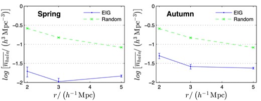
Average number density of neighbouring haloes, |$\overline{n_{{\rm halo}}}$|, with Mhalo > 1011 h− 1 M⊙ as a function of the sphere's radius around the EIGs or random galaxies, r, in which the density is averaged (calculated using Mill2).
3.9 Neighbourhood mass density
The mass density of neighbouring haloes, ρ, was analysed in both the Mill2 and Box160 simulations (each with its limiting Mhalo) within three spheres of radius r = 2, 3, 5 h−1 Mpc. Fig. 19 show the PDFs of ρ, calculated for r = 3 h−1 Mpc.

PDF of the mass density of neighbouring haloes, ρ, in a 3 h−1 Mpc radius sphere around the EIGs or random galaxies.
Fig. 19 shows that EIGs populate the low-ρ environments, while random galaxies populate both low- and high-ρ environments. The Spring sky region EIGs (left-hand panels) are generally located in lower ρ environments compared to the Autumn EIGs (right-hand panels). This is a result of the higher completeness of the Spring data set, given the assumption of an average composition of the large-scale structure (as discussed in Section 3.2).
All PDFs calculated using Box160 (bottom panels) are somewhat shifted to lower ρ compared to their Mill2 (top panels) parallels. This shift can be attributed mainly to the higher neighbouring halo mass limit of Box160, Mhalo ≥ 1.8 × 10¹⁰ h− 1 M⊙, versus Mhalo ≥ 109 h− 1 M⊙ for Mill2.
The fraction of Spring EIGs that reside in ρ < 0.25 × 10¹¹ h2 M⊙ Mpc− 3 environments (averaged on a 3 h−1 Mpc radius sphere) is 0.98 ± 0.01, whereas for Autumn EIGs it is 0.91 ± 0.02 (Mill2) or 0.988 ± 0.003 (Box160). This, versus 0.16–0.32 for the random samples. The fraction of Spring EIGs that reside in ρ > 1011 h2 M⊙ Mpc− 3 environments is 0.02 ± 0.01 (Mill2) or 0.001 ± 0.001 (Box160), while for Autumn EIGs it is 0.04 ± 0.02 (Mill2) or 0.002 ± 0.001 (Box160). This, versus 0.30–0.50 for the random samples. The ‘tail’ of the PDF of the random galaxies continues beyond 2 × 10¹¹ h2 M⊙ Mpc− 3. A fraction of 0.34 ± 0.01 (Mill2) or 0.16 ± 0.01 (Box160) of the random galaxies reside in ρ > 2 × 10¹¹ h2 M⊙ Mpc− 3 environments.
The average mass density of neighbouring haloes, |$\overline{\rho }$|, was also analysed. Fig. 20 shows the Mill2 results as a function of the sphere radius, r. The figure shows that |$\overline{\rho }$| for Spring EIGs is about one order of magnitude smaller than that of the random samples in spheres with radius in the range 2 < r < 5 h−1 Mpc. For the Autumn region, |$\overline{\rho }$| of the EIGs is three to four times smaller than that of the random samples in this range. The dependence of the EIGs’ |$\overline{\rho }$| on r is similar to that of random galaxies.
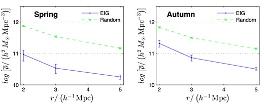
Average mass density of neighbouring haloes, |$\overline{\rho }$|, as a function of the sphere's radius around the EIGs or random galaxies, r, in which the density is averaged (calculated using Mill2).
3.10 Tidal acceleration
The tidal acceleration is defined here as the difference in gravitational acceleration exerted by neighbouring haloes, |$\boldsymbol {g}$|, per unit displacement, i.e. the divergence of this gravitational acceleration, |$\bigtriangledown \boldsymbol {g}$|. The total tidal acceleration, |$\bigtriangledown \boldsymbol {g}$|, that haloes within 5 h−1 Mpc exert on a galaxy was calculated for each mock EIG and random galaxy, with the approximation that the haloes’ masses are concentrated at their centre. Since |$\bigtriangledown \boldsymbol {g}$| varies by orders of magnitude, the PDFs were calculated for its logarithm, |$ {log}\left[ \left| \bigtriangledown \boldsymbol {g} \right| / \left( {\rm yr}^{-2} \right) \right]$|. The results are shown in Fig. 21.
![PDF of the tidal acceleration logarithm, ${\rm log} \left[ \left| \bigtriangledown \boldsymbol {g} \right| / \left( {\rm yr}^{-2} \right) \right]$, on EIGs or random galaxies.](https://oup.silverchair-cdn.com/oup/backfile/Content_public/Journal/mnras/456/1/10.1093/mnras/stv2662/2/m_stv2662fig21.jpeg?Expires=1749880396&Signature=UR266es996qe5LGhDa7kCRdXTqgghp-Y6k~kWfoCeEhQL-RUQk8kBuqxSh-oF7qijIxfmn6fpIzCxJ8Oh2AFhD65z1JxzHT~wDX43w1BGBqmcL2kwFCd3eeJ5HLAB9IVFTxdO17ALncygCklvBbk3IYObR-AVa2364MP2Ka8oS-Zyr40dcUA3s083c9a-hz7xNX4LEbsc8qR5-IQbrkz-GiglJjBgzMaVtdpVSZ0iXVfBA5eTaOiiqZge1CyHV0dSgzusAQs6d7K42aCxROc7Zhkq-feimrtm-sx3guXYdyLl0BNBAt00kFI-Mqc37S~7BGHRI8unwDL4JPWR~J~zg__&Key-Pair-Id=APKAIE5G5CRDK6RD3PGA)
PDF of the tidal acceleration logarithm, |${\rm log} \left[ \left| \bigtriangledown \boldsymbol {g} \right| / \left( {\rm yr}^{-2} \right) \right]$|, on EIGs or random galaxies.
Both simulations show that the average tidal acceleration, |$\bigtriangledown \boldsymbol {g}$|, of EIGs is about an order of magnitude smaller than that of random galaxies. The difference in |${\rm log} \left[ \left| \bigtriangledown \boldsymbol {g} \right| / \left( {\rm yr}^{-2} \right) \right]$| is larger for the Spring (−1.0 according to Mill2 and −1.4 according to Box160) compared to the Autumn (−0.8 according to Mill2 and −1.1 according to Box160). This again is the result of the lower completeness estimated for the Autumn region (see Section 3.2).
There is a discrepancy between the results of the Box160 simulation and those of Mill2. The average |${\rm log} \left[ \left| \bigtriangledown \boldsymbol {g} \right| / \left( {\rm yr}^{-2} \right) \right]$| of Box160 is lower than that of Mill2 by −1.5 for the random galaxies, and −1.8 for the EIGs. This discrepancy can be attributed mainly to the difference in the halo mass limit of the two data bases (Mhalo ≥ 1.8 × 10¹⁰h− 1 M⊙ for Box160 and Mhalo ≥ 109 h− 1 M⊙ for Mill2). However, this could also be a result of the Box160 calculation being based on FOF haloes and the Mill2 on gravitationally bound haloes, or due to the different cosmological parameters applied in the two simulations. If the halo mass limit has a strong effect, the actual |$\left| \bigtriangledown \boldsymbol {g} \right|$| is expected to be even higher than the Mill2 curve indicates.
The values of the tidal acceleration, |$\bigtriangledown \boldsymbol {g}$|, can be interpreted as indicating the typical time of induced change in the shape of objects by external interactions. For example, consider two nearby gas clouds with no relative motion in a constant |$\bigtriangledown \boldsymbol {g}$| tidal field. If the gravitation between these two clouds is negligible, the tidal field will drive the clouds apart, doubling their distance within |$t \cong 1.32 \left| \bigtriangledown \boldsymbol {g} \right|^{-0.5}$|. In general, the time in which a constant tidal acceleration field, |$\bigtriangledown \boldsymbol {g}$|, changes the shape of objects (or the distance between objects) is proportional to |$\left| \bigtriangledown \boldsymbol {g} \right|^{-0.5}$|.
The results of the tidal acceleration analysis, therefore, indicate that the time of induced change is ∼3 times larger, on average, for EIGs in comparison to random galaxies. This may have a significant effect on the star formation rate (SFR), if this time of scale change induced by neighbouring haloes is in the order of magnitude of typical shape change times induced by internal sources.
The discrepancy between the |$\left| \bigtriangledown \boldsymbol {g} \right|$|, calculated from Box160 data, and that calculated from Mill2 translates to a factor of 5–8 in this typical time of induced shape change (longer time for Box160). The actual shape change times are expected to be even shorter than those calculated using Mill2, if calculated with a mass limit lower than 109 h− 1 M⊙. A possible overestimate of the low-mass satellite haloes in the simulations (the missing satellite problem) might also affect the results, in which case the actual |$\left| \bigtriangledown \boldsymbol {g} \right|$| will be smaller than indicated by Mill2 and the typical time of induced shape change will be longer. This might have an effect on SFR of EIGs and random galaxies, where EIGs might be affected differently than random galaxies.
4 CONCLUSIONS
The simple isolation criterion (having no known neighbours within 3 h−1 Mpc), when applied to redshifts in the range 2000 < cz < 7000 km s−1 using NED and ALFALFA data, provides a sample of galaxies that are extremely isolated, compared to the general population.
Using cosmological simulations, we confirmed that the EIG-1 and EIG-2 subsamples are a subset of galaxies significantly more isolated than the general galaxy population. Apart from the low-density regions in which they reside, EIGs are characterized by normal mass haloes, which have evolved gradually with little or no major mergers or major mass-loss events. As a result of their low-density environments, the tidal acceleration exerted on EIGs is typically about one order of magnitude lower than the average tidal acceleration exerted on the general population of galaxies.
The level of contamination in the sample, i.e. the fraction of EIGs which are not in extremely isolated environments or which experienced strong interactions in the last 3 Gyr, was found to be 5–10 per cent. The Spring EIGs seem to be more isolated than the Autumn EIGs.
We have defined a major event as either a major merger (where the progenitors are at least 20 per cent of the mass of the merged halo) or a major mass-loss event (where a halo lost at least 10 per cent of its mass between successive simulation snapshots). We have found that this definition includes almost all interactions between haloes that are strong enough to significantly alter their MAHs. Haloes that did not experience major events in the last 10 Gyr accreted matter very similarly (when comparing after normalization with the current halo mass).
We have found that almost all low-mass haloes (Mhalo < 1010 h− 1 M⊙) that produced enough stars to be included in redshift surveys of the local Universe (Mg ≲ −14) experienced major events in their past. Therefore, Mill2 simulation results predict that samples of low-dark-mass galaxies are biased in the sense that they hardly include any galaxies that did not experience major events in their histories. We have found that EIGs are very unlikely to reside in such low-mass haloes, probably as a result of the fact that they hardly experience major events.
ALFALFA data are extremely useful in improving the sample's isolation level and in eliminating false positives, due to the redshift data it provides for low-luminosity galaxies with high H i masses. The EIG-1 subsample galaxies (EIGs which passed the isolation criterion with ALFALFA data, as well as with NED data) are significantly more isolated than the EIG-2 galaxies.
The properties of the EIG samples, derived from observations, will be described in a forthcoming paper (Spector & Brosch, in preparation).
We are grateful to Martha Haynes, Riccardo Giovanelli and the entire ALFALFA team for providing an unequalled H i data set. We are also grateful to Yehuda Hoffman, Stefan Gottlöber and Ofer Metuki for providing the Box 160 simulation data set. We are grateful to the anonymous referee for some constructive remarks that improved the paper.
This research has made use of the NASA/IPAC Extragalactic Database (NED) which is operated by the Jet Propulsion Laboratory, California Institute of Technology, under contract with the National Aeronautics and Space Administration. The Millennium-II Simulation data bases used in this work and the web application providing online access to them were constructed as part of the activities of the German Astrophysical Virtual Observatory (GAVO). Funding for SDSS-III has been provided by the Alfred P. Sloan Foundation, the Participating Institutions, the National Science Foundation and the US Department of Energy Office of Science. The SDSS-III website is http://www.sdss3.org/.
This criterion describes the most isolated subsample of EIGs studied here. Not all sample galaxies (EIGs) pass this isolation criterion (see Section 2.3).
In the FOF method (Davis et al. 1985), all particle pairs separated by less than a fraction, b, of the mean interparticle separation (linking length) are found. Each distinct subset of connected particles is then defined as an FOF group.
REFERENCES
APPENDIX A: EIG SPECIFIC DATA
This appendix contains general notes for some of the EIGs. It also discusses galaxies which were originally identified as isolated but were eventually not included in the sample.
A1 Notes for specific EIGs
EIG 1s-05
No optical counterpart could be identified for EIG 1s-05 (an ALFALFA object). In the WO images, no Hα emission was identified around the ALFALFA coordinates. Within 1 arcmin from the ALFALFA coordinates of EIG 1s-05, all galaxies detected by SDSS have g > 21.6, and none have spectroscopic redshifts. All GALEX detected objects in the same region have mFUV > 24 and mNUV > 21. EIG 1s-05 may, therefore, be a ‘dark galaxy’ with an extremely high H i-to-stellar mass ratio and a very low SFR. It may also be an ALFAFLA false detection, even though its SNR is 8.1 and it is considered a ‘code 1’ object, i.e. a source of SNR and general qualities that make it a nearly 100 per cent reliable detection (Haynes et al. 2011).
EIG 1s-09
SDSS DR10 shows an edge-on galaxy, SDSS J112157.63+102959.6, ∼13 arcsec east of the centre of EIG 1s-09. The angular size of SDSS J112157.63+102959.6 is similar to that of EIG 1s-09. Its magnitude is g = 18.6, compared to g = 16.9 of EIG 1s-09. The redshift of SDSS J112157.63+102959.6 is unknown. Although there is a possibility that SDSS J112157.63+102959.6 is a close neighbour of EIG 1s-09, this seems unreasonable, since tidal tails are neither visible in the SDSS images nor in deeper images taken by the authors (Spector & Brosch, in preparation).
EIG 1s-10
SDSS DR10 shows two objects at an angular distance of ∼6 arcsec from the centre of EIG 1s-10. One is north of EIG 1s-10, and is classified as a star by SDSS DR10. The second, classified as a galaxy, is south-west of EIG 1s-10. Both objects do not have measured redshifts. Although there is a possibility that one or both of these are galaxies merging with EIG 1s-10, this seems unreasonable, since tidal tails are neither visible in the SDSS images nor in deeper images taken by the authors (Spector & Brosch, in preparation).
EIG 1s-11
The only redshift measurement found for EIG 1s-11 is from Binggeli, Popescu & Tammann (1993) that quotes Hoffman et al. (1987). This is an H i measurement made at the Arecibo observatory. The H i profile for the galaxy was not published by Hoffman et al. (1987). It is possible that the measurement (4725 ± 10 km s−1) is a result of H i confusion, and that EIG 1s-11 is actually a part of the Virgo cluster.
EIG 1a-02
SDSS DR10 shows a galaxy, SDSS J005629.17+241913.3, ∼2 arcmin west of EIG 1a-02 with unknown redshift. The angular size of SDSS J005629.17+241913.3 is not very different from that of EIG 1a-02. Its magnitude is g = 16.6, compared to g = 17.0 of EIG 1a-02. Although there is a possibility that SDSS J005629.17+241913.3 is a close neighbour of EIG 1a-02, this seems unreasonable, since no tidal tails or other signs of interaction are visible in the SDSS images.
EIG 1a-04
Hα images of EIG 1a-04 showed strong star formation in LEDA 213033, a galaxy separated by 107 arcsec from EIG 1a-04 (Spector & Brosch, in preparation). Since LEDA 213033 has no measured redshift, its distance from EIG 1a-04 is unknown. The fact that it shows emission in the two narrow Hα filters used for the measurement (described in Spector & Brosch, in preparation) indicates that its redshift is cz ≅ 6000 ± 1500 km s−1. Therefore, the probability that it is less than 300 km s−1 away from EIG 1a-04 is estimated to be ∼10 per cent. No sign of interaction between EIG 1a-04 and LEDA 213033 was detected.
EIG 3s-06
This is the only EIG that passes the isolation criterion using the ALFALFA data set, but had neighbours closer than 3 h−1 Mpc in the NED data set. It was classified as part of subsample EIG-3s, because all of its NED neighbours are more than 2 h−1 Mpc away from it.
A2 Galaxies found in the search but not included in the sample
Two galaxies (CGCG 063-006 and UGC 09989) were first identified as EIGs but were later excluded from the sample, when neighbours closer than the 3 h−1 Mpc limit were identified for them in SDSS. In previous work (Spector 2015), these galaxies were referred to as EIG 2s-03 and EIG 3s-08 (respectively). For CGCG 063-006, a neighbour (SDSS J093248.11+121645.7) was found at a distance of 0.93 Mpc in redshift space. For UGC 09989, a neighbour (SDSS J154317.50+094155.8) was found at a distance of 1.24 Mpc in redshift space. The visible images of UGC 09989 show an extension to the north-west, which ends in a galaxy of smaller angular size. This extension seems to be material extracted from the galaxy, possibly by interaction with a neighbour galaxy. WISE images show this extension clearly in bands W1 and W2 (3.4 and 4.6 μm respectively).
Two objects (FGC 1647 and HIPASS J0835+14) were not included in the sample, because they were not found at their published coordinates. Data for FGC 1647 were published in the Flat Galaxy Catalogue (Karachentsev, Karachentseva & Parnovskij 1993). As advised by Igor Karachentsev, it does not appear in the Revised Flat Galaxy Catalogue (Karachentsev et al. 1999) possibly due to a mistake in coordinates. Data for HIPASS J0835+14 appear in the H i Parkes All Sky Survey catalogue (Wong et al. 2006). This object was not included in the sample since no counterpart was found for it in the optical images or in the ALFALFA catalogue.
Three other objects (CGCG 043-113, SDSS J084236.58+103313.9 and SDSS J140626.67+092132.5) were not included in the sample after the redshift quoted for them in NED was found to be wrong, and using redshift obtained from alternative sources many close neighbours were found for them. For all three galaxies, NED did not list sources for the redshift values it quotes. The accurate values obtained from alternative sources (SDSS DR10 for CGCG 043-113 and SDSS J084236.58+103313.9, and ALFALFA for SDSS J140626.67+092132.5) were significantly different. Using these more accurate values, CGCG 043-113 was found to have 28 neighbours in NED (and 23 in ALFALFA) closer than 3 h−1 Mpc, with the closest neighbour at a distance of 0.38 h−1 Mpc. SDSS J084236.58+103313.9 was found to have three neighbours in NED (and five in ALFALFA) closer than 3 h−1 Mpc. SDSS J140626.67+092132.5 was found to have 65 neighbours in NED (and 24 in ALFALFA) closer than 3 h−1 Mpc, with the closest neighbour at a distance of 0.15 h−1 Mpc.
The following galaxies were not included in the sample because of their unreliable redshift values.
SDSS J104658.12+132911.3 – For this galaxy, NED quotes the value 3605 ± 94 km s−1 from SDSS DR5 (Adelman-McCarthy et al. 2007), which is labelled with a warning status. Later SDSS releases list totally different values: z = 2.2 ± 0.6 with a warning status in SDSS DR7 (Abazajian et al. 2009), and z = 0.3 ± 0.6 in SDSS DR9 and DR10 (Eisenstein et al. 2011; Ahn et al. 2014). No other redshift measurement was found for this target in NED or in ALFALFA.
[PGH98] 1228+1241 – The uncertainty and source of the redshift measurement that NED quotes for this galaxy are not documented. The only reference that was found with a redshift measurement for this galaxy (Petrosian et al. 1998) quotes a significantly different value and does not list its uncertainty.
VIII Zw 202 – The only redshift measurement found for this galaxy is cz = 3604 ± 159 km s−1 (Drinkwater et al. 1996). With this large uncertainty, the isolation of the galaxy cannot be guaranteed.
SDSS J134517.15+112452.6 – SDSS is the only redshift source for this galaxy. SDSS DR7 measured cz = 5556 ± 206 km s−1, whereas SDSS DR8, DR9 and DR10 do not include its spectrum. With this uncertainty, the isolation of the galaxy cannot be guaranteed.
SDSS J153001.95+082550.9 – For this galaxy, NED quotes a redshift value from SDSS. However, different SDSS data releases measured significantly different values and issued warning statuses (SDSS DR6: cz = −141 ± 110 km s−1, SDSS DR7: cz = 2700 ± 113 km s−1 and SDSS DR10: cz = −79 ± 15). This could be due to a bright object close to the galaxy's line of sight that may contaminate the measured spectrum. No other redshift measurement was found for this target in NED or in ALFALFA.
UCM 2241+2431 – The only reference with a redshift measurement for this galaxy (Gallego et al. 1996) does not quote its uncertainty. Therefore, the isolation of the galaxy cannot be guaranteed.
2MASX J23420930+2640174 – For this galaxy, NED quotes only one redshift measurement: cz = 6038 ± 1001 km s−1 (Pinkney et al. 1993). Neither ALFALFA nor SDSS measured a redshift for it. With this extreme uncertainty, the isolation of the galaxy cannot be guaranteed, and its Hα emission measurement would not be accurate (because the transmittance of the Hα filter at the redshifted Hα line would not be known).
