


Abstract
The rapid analysis of ongoing gravitational microlensing events has been integral to the successful detection and characterization of cool planets orbiting low-mass stars in the Galaxy. In this paper, we present an implementation of search and fit techniques on graphical processing unit (GPU) hardware. The method allows for the rapid identification of candidate planetary microlensing events and their subsequent follow-up for detailed characterization.
1 INTRODUCTION
The OGLE (Udalski et al. 1994),1 MOA2 (Bond et al. 2002) and KMTNet3 wide-field surveys currently detect and alert in excess of 2000 microlensing events per year in the direction of the Galactic bulge. These events have an average time-scale of ∼ 22 d, but individual events can be as short as a few days or as long as a few hundred. A small subset of microlensing events produce anomalous short-duration signals lasting from a few hours to a few days due to the presence of one or more planets associated with the lens-star (which is typically an M dwarf). Almost all the planets that have been detected and characterized via microlensing have relied on high-cadence follow-up observations from various groups that include μFUN (Gould et al. 2006), RoboNet (Tsapras et al. 2009), PLANET (Albrow et al. 1996, 1998) and MiNDSTEp (Dominik et al. 2010).
The follow-up groups typically operate with small field-of-view cameras, capable of observing only one event at a time, so event selection can have a significant effect on the yield of microlensing planets. The follow-up groups typically focus on two classes of events. First, Griest & Safizadeh (1998) have shown that, given the presence of a planet orbiting a lens star, a trajectory having a low-impact parameter (i.e. a high magnification) is significantly more likely to intercept a central caustic and therefore produce an anomalous signal. Thus, events predicted to reach very high magnification are chosen for intensive observation over their peak magnification times. Secondly, events that are observed to be undergoing an anomaly are priority targets for follow-up. Unfortunately, this second category of anomalous events is dominated by binary stars, rather than star–planet microlensing.
In order to select events from this category for intensive follow-up, rapid preliminary analysis of in-progress events is necessary. In this paper, we describe a new graphics processing unit (GPU) based code designed for rapid analysis of ongoing microlensing events.
The layout of the paper is as follows. In Section 2, we describe briefly the GPU-computing architecture on which the code is based. In Sections 3–5, we present the algorithms and implementation details. Section 6 shows two examples of event analysis, and a summary is given in Section 7.
2 GPU ARCHITECTURE
A GPU is a common component found in most desktop computers, but only recently has the potential of these devices for general computation been realized, in a range of disciplines from sciences to finance (Gaikwad & Toke 2009; Sainio 2010; Isborn et al. 2011; Mashimo et al. 2013). By utilizing the large-scale parallelization ability of GPUs, increased performance can be achieved for some computational calculations if correctly incorporated. Most importantly, GPU code is generally inherently scalable, and increases in the number of GPU cores per device continues to outpace developments in CPU technology (see for instance; Vernardos & Fluke 2014).
For this code, we have adopted the compute unified device architecture (CUDA) extensions to the c language, developed by NVIDIA Corporation. A CUDA-enabled device can be thought of as a grid of processing units (CUDA cores) that can execute sets of instructions (threads) in parallel. Blocks of up to 1024 threads (on compute capability 2.0) can be coded to access an amount of shared memory, with different threads (within a block) able to access individual elements of an array. Blocks can execute on the GPU either sequentially or in parallel, depending on their size and the number of computing cores in the device. At the device level, groups of 32 threads within a block (warps) have hardware-enforced parallel execution. Blocks of threads and grids of blocks can have either 1-, 2- or 3-dimensional configurations (in CUDA compute capability 2.0 devices).
Additional to the shared memory (with fast read–write performance), threads have access to a slower read–write access global memory, and a hardware-optimized read-only texture memory. Both of these may be accessed by all threads, in all blocks of a single GPU function call. Texture memory is designed to store 2- and 3-dimensional arrays, and the computing architecture is designed for very rapid access to neighbouring pixels. This allows, for instance, very fast bilinear interpolation of an image stored in texture memory.
3 THE BINARY MICROLENSING MODEL
The point-source model for a microlensing event is rarely adequate for the majority of recognized binary microlensing events. In these cases, the source tends to pass close-to, or over, a lens caustic, which serves to resolve the source. To model such events, we must use a methodology that accounts for the finite source size. The two most common algorithms for this are contour integration via Stokes’ theorem (Gould & Gaucherel 1997; Bozza 2010) and various refinements of ray shooting maps (Kayser, Refsdal & Stabell 1986; Bennett & Rhie 1996; Dong et al. 2006). In Sections 4 and 5, we describe our strategy that is based on the magnification map approach.
4 COARSE GRID SEARCH
4.1 Magnification maps
Adopting Einstein-radius-normalized coordinates, set in the lens plane with the origin as the centre of mass of the lens and the lens masses lying on the z1-axis, a binary microlensing event may be described by seven basic parameters: d, the angular separation of the two lens components; q, the mass ratio of the lens components; u0, the distance of closest approach of the source to lens’ barycentre; ϕ, the trajectory angle of the source measured from the positive axis that passes through both lens components; t0, the time of closest approach; tE, the time for the source to move an angular distance of one Einstein radius; and ρ, the angular source radius.
At the highest level, we set up a 29 × 21 fixed grid in (log d, log q). For each (log d, log q) pair, we generate a point-source magnification map, by solving the fifth-order polynomial inversion of equation (2) for a uniform grid of source positions ζij. For this calculation, each GPU thread independently computes the magnification for a given pixel in the map. The map is then convolved on the GPU, by a number of radially symmetric source intensity profiles of different radii and fixed limb darkening (ΓI = 0.53). This produces a set of magnification maps corresponding to fixed ρ values. We have adopted seven values of ρ logarithmically spaced over (0.001, 1). Our tests have shown that on currently available hardware it is faster to recompute these maps from scratch than to load them into memory from hard disk storage. The magnification maps are loaded into GPU texture memory for the next stage of the analysis – a search over (u0, ϕ, ρ, t0, tE) space for each given (d, q).
4.2 Re-parametrizing u0
Since u0 is defined with respect to the centre of the binary lens, a search of trajectories in a magnification map over a grid of angles ϕ and impact parameters u0 is liable to miss small caustic structures that are located far from the centre. These small (planetary) caustics can be critical in identifying binary lenses that include a low-mass component. With this in mind, we replace a search over u0 with a search over fixed radial distances, r, from the central regions of caustics. These radial distances are scaled by the sizes of the caustics, as shown in Fig. 1.
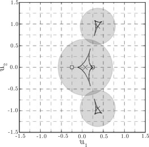
Example of an (r, ϕ) search space about the caustics of a d = 0.7, q = 0.5 binary. The coordinates (u1, u2) are positions in the lens plane in Einstein radius units relative to the mid-point of the lens masses. Lens masses are marked by ‘O’ symbols and the centres of the search spaces are marked by ‘X’.
We conduct a search over (t0, tE, ρ) for a fixed grid of (r, ϕ), where each (r, ϕ) pair is treated as a single block on the GPU. We refer to an (r, ϕ) pair as a trajectory. For this stage of the search, we use the simplex downhill method to locate a χ2 minimum. At each iteration of the downhill search, each GPU thread is used to compute the contribution to χ2 from a single observed data point. A given (ti, t0, tE) maps to a point (i) on a linear trajectory defined by (r, ϕ), through a given (d, q, ρ) map. Bilinear interpolation of the magnification maps stored in texture memory is used to retrieve the magnification A(ti) for the time of each data point.
4.3 Optimizations
There are several optimizations we make to improve the speed of the computation as follows.
We use the observed peak-to-baseline magnitude range of the microlensing event to infer a minimum magnification that needs to take place in order for a trial trajectory to be a viable solution. The magnification as a function of position along a trajectory is quickly extracted from the point-source map and discarded if it does not fulfil this minimum magnification criterion.
In cases where the light curve is obviously near in shape to that of a single lens (Paczyński), we use the estimated single lens parameters as starting points for (t0, tE) in the simplex.
In cases where the light curve has, or is expected to contain, more than one peak, we reject trajectories where the point-source map contains fewer than the specified number of peaks. Since we are using a fixed grid of (d, q, r, ϕ), we have pre-computed a library that specifies the number of peaks in each trajectory. A peak is considered to be any point on a trajectory where the magnification gradient changes from positive to negative.
- In non-Paczyński cases where we are able to specify the time of a single peak, t0 and tE are related bywhere tp is the input time of the peak from the data and Mp is the distance along the trajectory of the peak from t0 in units of Einstein radii. Mp is specified in our pre-computed library. For a given trajectory, we can then adjust t0 to best match the data in order to find our starting simplex parameters.(7)\begin{eqnarray} t_0 = t_{\rm p} - M_{\rm p} t_{\rm E}, \end{eqnarray}
- The optimum situation occurs where the times of multiple peaks can be provided. This allows t0 and tE to be solved analytically for each viable trajectory since, in addition to equation (7),where the tp, i are the set of specified times of peaks, and Mp, i are the pre-computed model peak times in units of Einstein radii. Again, we use these values as starting points for the simplex search.(8)\begin{eqnarray} t_{\rm E} = \frac{t_{p2} - t_{p1}}{M_{p2}-M_{p1}} , \end{eqnarray}
4.4 Results
The outcome of our coarse grid search is a set of viable regions of parameter space where we expect to find the global solution. Fig. 2 shows an example of coarse-search results projected on to (log d, log q) space. Because of the coarseness of the (log d, log q, r, ϕ) grid, it is unreasonable to adopt the single best solution thus far found as being the likely seed for the global solution. Thus, we generally choose a number of local minima from the coarse search for further analysis. At this time, we adopt the three best wide solutions (d ≥ 1) and narrow solutions (d < 1) as our seeds.
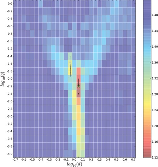
The log χ2 map in (log d, log q) space for OGLE-2003-BLG-0235. Overlaid arrows show the movement from seed solutions during the MCMC search.
5 REFINING SOLUTIONS
To refine our seed solutions, we employ a Markov Chain Monte Carlo (MCMC) search. For this part of our modelling, we discard the magnification map approach and instead compute magnifications for a given set of trial parameters using an image-centred ray shooting algorithm similar to that of Bennett (2010). The Markov chain sampling is implemented in the python language with CUDA c used to compute magnifications.
To implement our calculations on a GPU, we treat the epoch of each data point as a single block. Within a block, we use groups of threads to perform integrations over images, with each thread corresponding to different locations on an image.
Initially we compute the locations of the caustics corresponding to the current (d, q). This information is shared with all blocks (epochs). We then use 128 threads distributed over the caustic edges to establish the proximity of the source to its nearest caustic. For source-caustic distances greater than 10ρ, we use the point-source approximation for the magnification, otherwise we proceed with image-centred ray shooting calculations as follows.
Again using 128 threads distributed around the source boundary and its centre, we compute image positions for these source points. Resampling near the highest magnification points is performed in order to detect situations where a source is grazing a caustic. Starting from the centre of each image, a polar grid is iteratively expanded until it encompasses the entire image. Polar coordinates are used since images are often crescent shaped, approximately following the locus of the critical curves (see Fig. 3). Tests are incorporated to detect merged images.
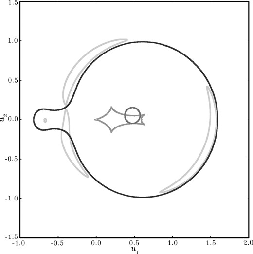
A finite source (dark central circle) passing over a caustic structure (five-pointed central structure), resulting in five images (lightest grey) that closely follow the edge of the critical curves (darkest grey). This example also shows the merging of two images that cross the critical curve due to the source being partially inside of the caustic structure.
We now integrate over each image with a weighting corresponding to the source intensity profile (found by inverse ray shooting). To deal with the numerical problems introduced by the fact that the source intensity is zero at the boundaries, we follow the second-order integration scheme given by Bennett (2010). Individual threads are used as grid points for the integration and we invoke parallel summation with loop unrolling for rapid computation.
5.1 Final solution with uncertainties
Upon completion of local area MCMCs, the best solution is chosen from the chain that produced the lowest final χ2 model, which we regard as being close to the global minimum. From this solution, the data errors are normalized by forcing χ2 per degree of freedom for each source of data to unity. Although statistically undesirable, normalizing errors bars in this way prevents bias due to poorly estimated uncertainties in particular data sources. We then use the sampler EMCEE (Foreman-Mackey et al. 2013) along with CUDA image-centred ray shooting to determine our final solution and parameter covariances.
5.2 Higher order effects
The inclusion of higher order effects such as parallax and orbital motion can be incorporated in the GPU kernel to modify the source and lens positions when performing inverse ray shooting, at minimal computational cost. However, new challenges arise when incorporating these effects into a search strategy whilst maintaining high performance. Parallax (and xallarap) could, in principle, be added to the current grid search strategy, as they only affect the interpolated source trajectory. The inclusion of orbital motion at this stage is not possible since multiple (d, q) magnification maps per trajectory would be required. These higher order effects are typically only considered if necessary after the original seven parameters have been determined, at which point they are incorporated into the EMCEE search, which uses image-centred ray shooting.
6 EXAMPLES
As demonstrations and verification of our code, we present results below for two well-known events that have been previously analysed.
6.1 OGLE-2003-BLG-0235
This was the first microlensing event in which a planet was discovered, see Bond et al. (2004). It has more recently been reanalysed by Bennett (2010). Data were taken by the OGLE and MOA survey telescopes that show a moderate magnification microlensing event (A0 ∼ 5.5) that peaked at around JD 245 2847. The event shows a caustic passage that lasted for ∼7 d from JD 245 2834. In Table 1, we show the solutions found by Bond et al. (2004).
Binary lens seven parameter model maximum likelihood solutions of MOA-2003-BLG-0053/OGLE-2003-BLG-0235, showing planetary solutions and the best non-planetary model (Bond et al. 2004) and from our code, based on EMCEE runs using error-normalized data.
| Bond et al. (2004) solutions | This paper | ||||
|---|---|---|---|---|---|
| Best | Early caustic | Best | Wide | Close | |
| Parameter | planetary | planetary | non-planet | planetary | planetary |
| d | 1.120 ± 0.007 | 1.121 | 1.090 | 1.117 | 0.9143 |
| q(×10−3) | |$3.9 ^{+1.1 }_{ -0.7}$| | 7.0 | 30.0 | 6.5 | 11.5 |
| ρ(×10−4) | 9.6 ± 1.1 | 10.4 | 8.8 | 9.9 | 8.6 |
| u0 | 0.133 ± 0.003 | 0.140 | 0.144 | 0.138 | 0.154 |
| ϕ | 0.7644 ± 0.0024 | 0.6789 | 0.1379 | 0.677 | 3.25 |
| t0 | 2848.06 ± 0.13 | 2847.90 | 2846.20 | 2847.91 | 2850.02 |
| tE | 61.5 ± 0.18 | 58.5 | 57.5 | 59.5 | 56.8 |
| χ2/dof | 1508.19/1374 | 1597.67/1374 | |||
We have modelled the event using the OGLE and MOA data from Bond et al. (2004) that have been made available through the NASA Exoplanet Archive.4 The entire OGLE data set of 285 points was used, while the MOA data set was reduced from 1152 data points down to 1089 by rejecting points with very large uncertainties. We specified a minimum base–peak light curve amplitude of 2.0 mag, and demanded that solutions contained at least three light curve peaks, with two of these located near JD 245 2842.08 (the caustic exit) and JD 245 2848.0 (the central peak). The χ2 map from our initial grid search is shown in Fig. 2. This initial search took 59 min using an NVIDIA Tesla C2075 GPU card. MCMC models using the image-centred ray shooting procedures discussed in Section 5 were then started from the three best close (d < 1) and wide (d > = 1) solutions. Well-converged solutions, using a total of 4000 iteration steps per chain were obtained for these six chains in around 1.85 h. Arrows on Fig. 2 indicate the movement of solutions during the MCMC iterations. In Table 1, we show the parameters of our two best solutions compared with those found by Bond et al. (2004). Our final solution, incorporating normalized data uncertainties, and with parameter uncertainties generated using EMCEE, is given in Table 2 and Fig. 4, and is the same as the best solutions found previously.
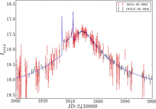
Final fitted light curve for the marginalized wide solution of OGLE-2003-BLG-235.
Final seven parameter binary lens model solutions of OGLE-2003-BLG-0235 from error-normalized data. These are the marginalized posterior mean and standard deviation for each parameter.
| Marginalized | Marginalized | |
|---|---|---|
| Parameter | wide solution | close solution |
| d | 1.120 ± 0.004 | 0.915 ± 0.002 |
| q(×10−3) | 6.3 ± 0.6 | 11.7 ± 1.0 |
| ρ(×10−4) | 10.0 ± 1.2 | 8.98 ± 0.71 |
| u0 | 0.137 ± 0.004 | 0.154 ± 0.005 |
| ϕ | 0.695 ± 0.024 | 3.24 ± 0.02 |
| t0 | 2847.91 ± 0.11 | 2850.02 ± 0.13 |
| tE | 59.8 ± 1.6 | 56.8 ± 1.5 |
This analysis also serves as a performance comparison with the method of Bennett (2010), who achieved the same ‘Best planetary’ solution of Table 1 by searching a restricted parameter space of slightly more than 70 000 parameter sets in 5 h and 14 min. Using our methods, we determined our six best coarse solutions by exploring an unrestricted parameter space of 8197 199 parameter sets in 59 min. This includes the time for each parameter set to potentially perform a simplex downhill search of up to 5000 steps over (t0, tE, ρ) Including the subsequent six MCMC explorations, the analysis explored between 8 million and 40 million parameter trials in 2 h and 50 min.
6.2 OGLE-2012-BLG-0406
This is an example of an event detected and monitored by the OGLE IV survey group, with intensive follow-up observations by several other groups. Following detection in 2012 April, the event was predicted to have a low peak magnification and was considered low priority for follow-up. An anomalous brightening was recognized in early July, prompting monitoring by the PLANET and microFUN groups using telescopes at the South African Astronomical Observatory (SAAO) and the Cerro Tololo Inter-American Observatory (CTIO) respectively. Following a peak in the light curve on July 5 and recognition by C. Han that the light curve was probably planetary in nature, several other telescopes began to intensively monitor the event.
The light curve has been modelled by Poleski et al. (2014) using only OGLE survey telescope data, and Tsapras et al. (2014) who used data from 10 separate observing sites. Both of these papers used a similar initial search routine, with a few differences in the filtering and error scaling of the data used. Poleski et al. (2014) assumed a limb-darkening coefficient of ΓI = 0.353 whereas Tsapras et al. (2014) assumed ΓI = 0.53.
Due to the deviations from a point-source light curve being of short time-scale on the shoulder of a Paczyński curve, it is safe to conclude that the cause of the anomaly is from the source passing close to a central caustic. In such a case, the single lens parameters of u0, t0, and tE (which can be determined with relative ease) are similar to the matching parameters of the binary lens model. Tsapras et al. (2014) used this information to perform a hybrid grid search of d, q, and ϕ, where u0, t0, tE, and ρ are minimized using MCMC methods. The grid was searched between the limits of −1 ≤ log10(d) ≤ 1, −5 ≤ log10(q) ≤ 1, and 0 ≤ ϕ ≤ 2π with the aim to locate all areas of local minimum, before further refinement by narrowing the grid search parameter space. Finally a χ2 optimization in all seven parameters was performed in each local minimum to determine the best solution. The Tsapras et al. (2014) and Poleski et al. (2014) binary lens model solutions are shown in Table 3.
Seven parameter binary lens model solutions for event OGLE-2012-BLG-0406.
| All data | OGLE only | |||
|---|---|---|---|---|
| Parameter | Tsapras et al. (2014) | This paper | Poleski et al. (2014) | This paper |
| d | 1.346 ± 0.001 | 1.3466 ± 0.0009 | 1.3500 ± 0.0016 | 1.3505 ± 0.0019 |
| q(×10−3) | 5.33 ± 0.04 | 5.32 ± 0.04 | 5.78 ± 0.08 | 5.78 ± 0.09 |
| ρ(×10−2) | 1.103 ± 0.008 | 1.086 ± 0.011 | 0.98 ± 0.05 | 0.95 ± 0.05 |
| u0 | 0.532 ± 0.001 | 0.5314 ± 0.0013 | 0.5425 ± 0.0022 | 0.540 ± 0.003 |
| ϕ | 0.852 ± 0.001 | 0.8555 ± 0.0013 | 0.8653 ± 0.0016 | 0.8654 ± 0.0017 |
| t0 | 6141.63 ± 0.04 | 6141.46 ± 0.04 | 6141.59 ± 0.03 | 6141.43 ± 0.05 |
| tE | 62.37 ± 0.06 | 62.52 ± 0.12 | 62.63 ± 0.16 | 62.52 ± 0.19 |
We have used our code as described in Sections 3–5 above to fit the data sets used by Poleski et al. (2014) (OGLE only) and by Tsapras et al. (2014). The Tsapras et al. (2014) data consist of 81 observations from CTIO I band Chile (microFUN), 181 from Robonet Siding Spring Australia, 83 from Robonet Haleakala Hawaii, 131 from Robonet La Palma, 210 from Canopus Observatory Tasmania Australia (PLANET), 180 from Wise Observatory Israel, 473 from Danish 1.5 m La Silla Chile (MiNDSTEp), 3013 from OGLE Las Campanos Chile, 1856 from the B&C 60 cm Mt John New Zealand (MOA), and 226 from SAAO 1 m South Africa (PLANET). Our initial grid searches located the same areas of local minima as Poleski et al. (2014) and Tsapras et al. (2014). Our subsequent MCMC refinements using image-centred ray shooting determined the same minima as those previous solution as given in Table 3. The fitted multi-data set light curve is shown in Fig. 5.
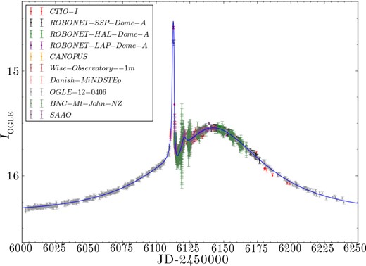
Final fitted light curve for OGLE-12-BLG-406
7 SUMMARY
In this paper, we have described a fast method for fitting binary gravitational microlensing events. The code is written in CUDA c and python, and the computationally intensive parts are run on massively parallel GPU hardware. The code will scale naturally to higher performance as GPU technology evolves.
As part of our algorithms, we introduce several optimizations that improve the ability to detect features due to small caustics and the speed of execution. Results from our ongoing analysis of current events are reported through our website.5
MDA thanks the Department of Astronomy, University of Wisconsin-Madison, for hospitality during the writing of this paper. We thank NVIDIA Corporation for supporting our work.
REFERENCES
