Stability of metal-rich very massive stars

Basic properties of our ZAMS models.

M/M_⊙	L/L_⊙	R/R_⊙	T_eff (K)	X_c
10.0	5.118 × 10³	3.922	24 688	0.727
21.5	4.841 × 10⁴	5.998	34 983	0.727
46.4	2.962 × 10⁵	9.279	44 236	0.727
100	1.244 × 10⁶	15.27	49 360	0.729
215	4.054 × 10⁶	30.88	46 638	0.726
464	1.135 × 10⁷	75.29	38 635	0.728
938	2.686 × 10⁷	274.3	25 106	0.727

M/M_⊙	L/L_⊙	R/R_⊙	T_eff (K)	X_c
10.0	5.118 × 10³	3.922	24 688	0.727
21.5	4.841 × 10⁴	5.998	34 983	0.727
46.4	2.962 × 10⁵	9.279	44 236	0.727
100	1.244 × 10⁶	15.27	49 360	0.729
215	4.054 × 10⁶	30.88	46 638	0.726
464	1.135 × 10⁷	75.29	38 635	0.728
938	2.686 × 10⁷	274.3	25 106	0.727

Table 1.

Basic properties of our ZAMS models.

M/M_⊙	L/L_⊙	R/R_⊙	T_eff (K)	X_c
10.0	5.118 × 10³	3.922	24 688	0.727
21.5	4.841 × 10⁴	5.998	34 983	0.727
46.4	2.962 × 10⁵	9.279	44 236	0.727
100	1.244 × 10⁶	15.27	49 360	0.729
215	4.054 × 10⁶	30.88	46 638	0.726
464	1.135 × 10⁷	75.29	38 635	0.728
938	2.686 × 10⁷	274.3	25 106	0.727

M/M_⊙	L/L_⊙	R/R_⊙	T_eff (K)	X_c
10.0	5.118 × 10³	3.922	24 688	0.727
21.5	4.841 × 10⁴	5.998	34 983	0.727
46.4	2.962 × 10⁵	9.279	44 236	0.727
100	1.244 × 10⁶	15.27	49 360	0.729
215	4.054 × 10⁶	30.88	46 638	0.726
464	1.135 × 10⁷	75.29	38 635	0.728
938	2.686 × 10⁷	274.3	25 106	0.727

Once the star has reached its ZAMS phase, the model is saved and the data are analysed with the adipls package (Christensen-Dalsgaard 2008), which computes adiabatic pulsational modes given one-dimensional stellar models. The output from adipls is a set of eigenfrequencies and corresponding mode shapes in the form of radial displacements from equilibrium. We use these outputs in our own routine, which finds mode frequencies and shapes without the adiabatic assumption. We turn to this method now.

2.2 Non-adiabatic analysis

For the purpose of analysing the pulsational modes in a non-adiabatic framework, we began by adopting the method outlined in Castor (1971), with mass fraction as the independent variable, and a Henyey-type relaxation scheme for finding the eigenfrequencies. Despite extensive efforts and algorithmic variations, this did not give numerically stable results for the growth rate of the fundamental mode, possibly because of the many orders of magnitude separating the dynamical and thermal time-scales in the core, and the enormous radial variation in the ratio of these time-scales through the star.

We therefore adopted a sort of shooting method designed for very stiff equations (Appendix A). The basic linearized equations are

\begin{eqnarray} \frac{\mathrm{\partial} }{\mathrm{\partial} r} \delta P_\mathrm{gas}&=& \rho \left[\omega ^2\delta r + g_{\rm rad}\left(\frac{\delta \kappa }{\kappa }+\frac{\delta L_\mathrm{rad}}{L_\mathrm{rad}}\right) + 4g_{\rm eff}\frac{\delta r}{r}\right], \end{eqnarray}

(1a)

\begin{eqnarray} r^{-2}\frac{\mathrm{\partial} }{\mathrm{\partial} r}(r^2\delta r) &=& -\frac{\delta \rho }{\rho }, \end{eqnarray}

(1b)

\begin{eqnarray} \frac{\mathrm{\partial} }{\mathrm{\partial} r}\delta P_\mathrm{rad}&=& -\rho g_{\rm rad}\left(\frac{\delta \kappa }{\kappa }+\frac{\delta L_\mathrm{rad}}{L_\mathrm{rad}}-4\frac{\delta r}{r}\right), \end{eqnarray}

(1c)

\begin{eqnarray} \frac{\mathrm{\partial} }{\mathrm{\partial} r}\delta L &=& \text{i}\omega 4\pi r^2\rho T\delta S + 4\pi r^2\rho \frac{\delta \epsilon }{\epsilon }. \end{eqnarray}

(1d)

Here |$g_{\rm rad}=\kappa L_\mathrm{rad}/4\pi r^2 c$| is the radiative force per unit mass, g_eff = GM_r/r² − g_rad is the residual between the gravitational and radiative accelerations, δ represents Lagrangian perturbation (first-order variation at fixed interior mass), and all other symbols have their usual meaning. We define dimensionless linearized variables

\begin{equation} y_0\equiv \frac{\delta r}{r},\quad y_1\equiv \frac{\delta \rho }{\rho }, \quad y_2\equiv \frac{\delta T}{T},\quad y_3\equiv \frac{\delta L_\mathrm{rad}}{L}. \end{equation}

(2)

Notice that L not L_rad appears in the denominator of y₃.

In principle δL = δL_rad + δL_conv. However, since there is no generally accepted prescription for time-dependent convective luminosity – especially in the radiation-pressure-dominated regime – we adopt δL_conv = 0 (‘frozen convection’). Nor have we allowed for a turbulent convective viscosity in the linearized momentum equation (1a).

Then in terms of our dimensionless variables, with primes for d/dr and writing f ≡ L_rad/L, κ_T = (∂ln κ/∂ln T)_ρ, κ_ρ = (∂ln κ/∂ln ρ)_T, and similarly for ϵ_T and ϵ_ρ, equations (1) become

\begin{eqnarray} ry_0^{\prime } &=& -3y_0-y_1, \end{eqnarray}

(3a)

\begin{eqnarray} y_1^{\prime }+y_2^{\prime } &=& \frac{\rho }{P_\mathrm{gas}}[\omega ^2r y_0+g_{\rm rad}(\kappa _\rho y_1 +\kappa _Ty_2+f^{-1} y_3)\nonumber \\ && +\;g_{\rm eff}(4y_0+y_1+y_2)], \end{eqnarray}

(3b)

\begin{eqnarray} y_2^{\prime } &=& -\frac{\rho g_{\rm rad}}{4P_\mathrm{rad}}[\kappa _\rho y_1+\kappa _Ty_2 +f^{-1}y_3-4y_0-4y_2], \end{eqnarray}

(3c)

\begin{eqnarray} ry_3^{\prime } &=& \frac{4\pi r^3\rho }{L}\lbrace \text{i}\omega C_VT[y_2-(\Gamma _3-1)y_1]\nonumber \\ && +\;\epsilon (\epsilon _\rho y_1 +\epsilon _Ty_2 - y_3)\rbrace . \end{eqnarray}

(3d)

The system of equations is closed by choosing four boundary conditions. Physically, one expects δr = δL = δL_rad = 0 at r = 0. This does not require y₀ or y₃ to vanish at the centre, but from the first of equations (3), one sees that non-singular behaviour requires

\begin{equation} 3y_0+y_1\rightarrow 0\mbox{ as }r\rightarrow 0. \end{equation}

(4)

Similarly, regularity of the last of equations (3) implies

\begin{eqnarray} \frac{{\rm i}\omega C_VT}{\epsilon }[y_2-(\Gamma _3-1)y_1]+ \epsilon _\rho y_1 +\epsilon _Ty_2 - y_3\rightarrow 0\mbox{ as }r\rightarrow 0.\nonumber\\ \end{eqnarray}

(5)

The factor in front of the square brackets is ∼t_KH/t_dyn ≫ 1 if |$\omega \sim t_{\rm dyn}^{-1}$|⁠, so to a first approximation the behaviour near the origin is adiabatic, δ ln T ≈ (Γ₃ − 1)δ ln ρ. But since we are interested in growth or decay rates |$\omega _I\sim t_\mathrm{KH}^{-1}$|⁠, we use equation (5) as written.

The outer heat equation requires a more general analysis than is given by Castor, as the equations in that work only hold under the assumption that radiation pressure is negligible compared to gas pressure at the outer boundary. This condition clearly does not hold for very massive stars. We therefore turn to the equation for radiation pressure in the Eddington approximation:

\begin{equation*} P_\mathrm{rad}= \frac{F}{c} \left(\tau + \frac{2}{3}\right), \end{equation*}

where F is the radiative flux and τ is the optical depth at the location being considered. In more familiar variables,

\begin{equation} P_\mathrm{rad}= \frac{L_\mathrm{rad}}{4\pi r^2c} \left(\frac{\kappa \Delta m}{4\pi r^2} + \frac{2}{3}\right), \end{equation}

(6)

where Δm is the mass exterior to the point being considered, if the density scale height is ≪r. Linearizing yields

\begin{equation*} \frac{\delta P_\mathrm{rad}}{P_\mathrm{rad}} = \frac{\delta L_\mathrm{rad}}{L} - 4 \left(\frac{\tau +1/3}{\tau +2/3}\right) \frac{\delta r}{r} + \left(\frac{\tau }{\tau +2/3}\right) \frac{\delta \kappa }{\kappa }, \end{equation*}

or in dimensionless variables,

\begin{eqnarray} {-}4\left(\tau +\frac{1}{3}\right)y_0 +\tau \kappa _\rho y_1 + \tau \kappa _Ty_2 +\left(\tau +\frac{2}{3}\right)(y_3-4y_2)=0. \nonumber\\ \end{eqnarray}

(7)

We replace L_rad with L here because in practice the model extends far enough into the tenuous atmosphere as to make the contribution of L_conv negligible.

The outer momentum equation is closed as follows. The total pressure at a point near the surface, under a mass Δm and at a radius r, is

\begin{equation} P = \frac{\Delta m}{4\pi } \left(\frac{\ddot{r}}{r^2} + \frac{GM}{r^4}\right) + \frac{L}{6\pi cr^2}, \end{equation}

(8)

if the mass shell Δm is thin and effectively hydrostatic in its accelerated frame. The last term in equation (8) is the radiation pressure extrapolated to the outer surface of the shell, where τ = 0. Subtracting equation (6) from equation (8) yields

\begin{equation} P_\mathrm{gas}= \frac{\Delta m}{4\pi } \left(\frac{\ddot{r}}{r^2} + \frac{GM}{r^4} - \frac{\kappa L_\mathrm{rad}}{4\pi r^4c}\right). \end{equation}

(9)

Perturbing this yields

\begin{equation*} \frac{\delta P_\mathrm{gas}}{P_\mathrm{gas}} = -\frac{\delta r}{r} \left(4 + \frac{\omega ^2r^3}{\beta GM}\right) - \frac{1-\beta }{\beta } \left(\frac{\delta L}{L} + \frac{\delta \kappa }{\kappa }\right), \end{equation*}

or equivalently,

\begin{eqnarray} \left(4 + \frac{\omega ^2 R^3}{\beta GM}\right)y_0 &+& \frac{1-\beta }{\beta }(y_3 + \kappa _\rho y_1 + \kappa _Ty_2)\nonumber\\ &-& y_1-y_2 = 0, \end{eqnarray}

(10)

where β is defined in terms of the Eddington luminosity |$L_\mathrm{Edd}= 4\pi GMc/\kappa$| by L = (1 − β)L_Edd.

3 THE SHELF

When mesa evolves massive stars with non-negligible metallicity, it generically produces an extended envelope outside the polytropic core of the star, as shown in Fig. 2. This extremely diffuse region, which is incipient in the 46 M_⊙ model but prominent in those above 100 M_⊙, occupies a progressively larger fraction of the star's radius but a minute fraction of its mass (ΔM_shelf ≈ 3 × 10⁻⁶M for the 938 M_⊙ model). It is overwhelmingly dominated by radiation pressure, much more so than the stellar core. Because of its slowly radially varying temperature and density, we call this region the ‘shelf’, although the density profile is actually inverted in its outermost part (Fig. 2). The opacity in the shelf rises above the electron-scattering value. Since hydrostatic equilibrium limits the radiative part of the luminosity to the value that just balances gravity, |$L_\mathrm{rad}= 4\pi GM_{\ast }c/\kappa (\rho , T)$|⁠, and since the luminosity is near-Eddington, the balance of the luminosity (up to half, in our most massive model) is carried by inefficient convection that approaches the adiabatic sound speed, i.e. the sound speed based on total rather than gas pressure. A similar shelf has been observed in models of Wolf–Rayet stars and attributed to a bump in the iron opacity at temperatures ∼1–2 × 10⁵ K (Gräfener, Owocki & Vink 2012, and references therein).

Figure 1.

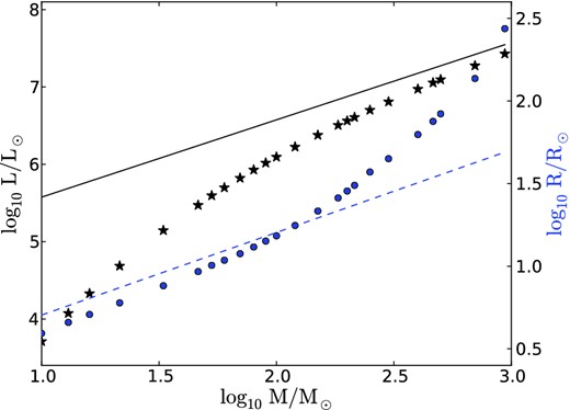
Luminosity (star symbols, left-hand scale) and photospheric radius (circles, right-hand scale) versus stellar mass for our mesa models. Thin solid line is the Eddington limit for this composition (Y = 0.25, Z = 0.02). Thin dashed line shows R ∝ M^1/2, as would be expected for homologous radiation-pressure-dominated models.

Figure 2.

Density (solid line, left-hand ordinate) and temperature (dashed line, right-hand ordinate) in our 938 M_⊙ model. Grey shading indicates convective regions. Dot–dashed line is the density profile of an n = 3 polytrope scaled according to equation (9) of Goodman & Tan (2004).

$Left-hand axis, red curve: fraction of luminosity carried by radiative diffusion in the 938 M⊙ model. Right-hand axis, blue curve: Bernoulli ‘constant’ normalized by mass and radius at the base of the shelf.$

Figure 3.

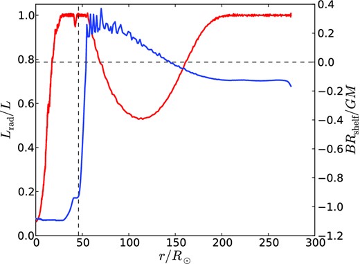
Left-hand axis, red curve: fraction of luminosity carried by radiative diffusion in the 938 M_⊙ model. Right-hand axis, blue curve: Bernoulli ‘constant’ normalized by mass and radius at the base of the shelf.

mesa uses OPAL radiative opacities (Iglesias & Rogers 1996) in the density and temperature regime relevant to the shelf. We employ the so-called Type 1 opacities (carbon and oxygen abundances not determined independent of metallicity) with ‘solar’ relative abundances as defined by Grevesse & Noels (1993). See Paxton et al. (2011), section 4.3, for more details.

In fact, the shelf might be replaced by a radiatively driven wind if the constraint of hydrostatic equilibrium were relaxed. This is suggested by the fact that the Bernoulli ‘constant’

\begin{equation} B = u + \frac{1}{2} v^2 + \frac{P}{\rho } + \Phi \end{equation}

(11)

becomes positive in the lower part of the shelf (Fig. 3), though it changes sign once more in the outer convective regions. Here u is the internal energy per unit mass, and v is the mean radial velocity, which of course vanishes in these hydrostatic models, and Φ(r) is the gravitational potential, defined to vanish as r → ∞. The kinetic energy of the convection would further increase B. These regions being strongly non-adiabatic, however, B > 0 does not guarantee a successful wind.

For a precise definition of the base of the shelf, we use the radius or mass fraction corresponding to the local minimum in the pressure scale height, H_P. For the model shown in Fig. 2, this is R_shelf = 46.3 R_⊙. Within our suite of models, such a minimum occurs only for M ≳ 50 M_⊙.

4 RESULTS

4.1 Adiabatic calculations

First we describe the results obtained using adipls. The seven lowest frequency modes for our 464 M_⊙ model are shown in Fig. 4. Weighting the displacement δr by ρ^1/2r shows where the energy of the mode is concentrated, in that ω² times the integral of the square of the plotted quantity gives the total energy.

Figure 4.

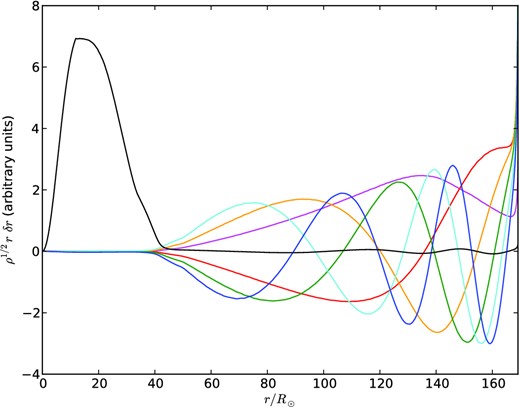
Plot of the lowest frequency adiabatic modes for the 464 M_⊙ model. The curves show the square root of the mode kinetic energy per unit length, normalized independently. The modes have radial mode number n equal to 1 (red), 2 (orange), 3 (green), 4 (cyan), 5 (blue), 6 (magenta), or 7 (black), only the latter of which is not evanescent in the core.

Of particular note is that the first six modes discovered by adipls are trapped in the shelf. The seventh mode is the true fundamental: its energy is concentrated in the core, where it has no nodes other than the centre, and it has an antinode at the base of the shelf (see Section 3). Some readers may object to our use of the term ‘fundamental’ for a mode that has multiple radial nodes. The adiabatic linearized problem is of Sturm–Liouville type, with orthogonal eigenfunctions having interleaved nodes. But the non-adiabatic problem is quite different. As Fig. 5 and Table 2 illustrate, the adiabatic and non-adiabatic versions of the fundamental (as we define it) are very similar – and both nodeless – in the core, and have nearly equal real parts of their eigenfrequencies, but can have different numbers of nodes in the shelf (11 and eight, respectively, for the real parts of the eigenfunctions shown in Fig. 5). Thus classification on the basis of numbers of nodes is not helpful in establishing a correspondence between the adiabatic and non-adiabatic eigenfunctions. Perhaps some other term such as ‘basic’ could be substituted for ‘fundamental’, but we feel that the latter is physically justified in this application.

Figure 5.

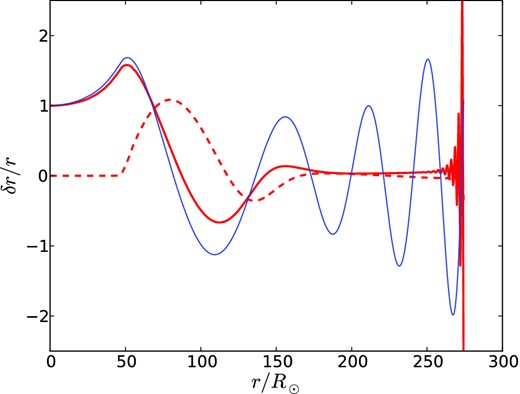
Fundamental radial mode at 938 M_⊙. Thin blue line: adiabatic displacement eigenfunction. Red lines: real (solid) and imaginary (dashed) parts of the fully non-adiabatic displacement eigenfunction. Eigenfunctions are not multiplied by r²ρ^1/2, in order to emphasize behaviour in the shelf (r > 46 R_⊙).

Table 2.

Periods and growth rates of fundamental radial mode. Negative growth rates indicate stability. Note 1 Md ≡ 10⁶ d.

M	Period	Growth rate (Md⁻¹)
(M_⊙)	(d)	ϵ	κ	Total	Convec.	No shelf
10	0.0905	−22.4	41.0	41.1	41.1	–
21.5	0.1391	−6.94	−10.3	−9.64	−9.68	–
46.4	0.2172	−3.01	−7.93	−6.33	−6.50	–
100	0.3279	−3.12	−2.37	+0.44	0.015	−1.73
215	0.4947	−19.5	−5.15	+9.28	8.45	+1.22
464	0.7253	−5.49	−11.1	−5.92	−7.19	+3.26
938	1.0435	−9.87	−15.5	−10.6	−11.9	+3.69

M	Period	Growth rate (Md⁻¹)
(M_⊙)	(d)	ϵ	κ	Total	Convec.	No shelf
10	0.0905	−22.4	41.0	41.1	41.1	–
21.5	0.1391	−6.94	−10.3	−9.64	−9.68	–
46.4	0.2172	−3.01	−7.93	−6.33	−6.50	–
100	0.3279	−3.12	−2.37	+0.44	0.015	−1.73
215	0.4947	−19.5	−5.15	+9.28	8.45	+1.22
464	0.7253	−5.49	−11.1	−5.92	−7.19	+3.26
938	1.0435	−9.87	−15.5	−10.6	−11.9	+3.69

Table 2.

Periods and growth rates of fundamental radial mode. Negative growth rates indicate stability. Note 1 Md ≡ 10⁶ d.

M	Period	Growth rate (Md⁻¹)
(M_⊙)	(d)	ϵ	κ	Total	Convec.	No shelf
10	0.0905	−22.4	41.0	41.1	41.1	–
21.5	0.1391	−6.94	−10.3	−9.64	−9.68	–
46.4	0.2172	−3.01	−7.93	−6.33	−6.50	–
100	0.3279	−3.12	−2.37	+0.44	0.015	−1.73
215	0.4947	−19.5	−5.15	+9.28	8.45	+1.22
464	0.7253	−5.49	−11.1	−5.92	−7.19	+3.26
938	1.0435	−9.87	−15.5	−10.6	−11.9	+3.69

M	Period	Growth rate (Md⁻¹)
(M_⊙)	(d)	ϵ	κ	Total	Convec.	No shelf
10	0.0905	−22.4	41.0	41.1	41.1	–
21.5	0.1391	−6.94	−10.3	−9.64	−9.68	–
46.4	0.2172	−3.01	−7.93	−6.33	−6.50	–
100	0.3279	−3.12	−2.37	+0.44	0.015	−1.73
215	0.4947	−19.5	−5.15	+9.28	8.45	+1.22
464	0.7253	−5.49	−11.1	−5.92	−7.19	+3.26
938	1.0435	−9.87	−15.5	−10.6	−11.9	+3.69

adipls also reports the frequencies of these modes, which are of course real in the adiabatic approximation. The corresponding periods, 2π/ω, of the fundamental modes differ only in the third or fourth significant digit from the values shown in the second column of Table 2 for the fully non-adiabatic fundamental modes.

4.2 Non-adiabatic calculations

In the linear equations, non-adiabaticity arises from two primary mechanisms. The nuclear heating rate per unit mass, ϵ, is sensitive to density and even more so to temperature. The strongly positive value of the logarithmic temperature derivative ϵ_T (≈12 near the centre of the 938 M_⊙ model) tends to add entropy during the compressive phase of the pulsation cycle when δT > 0, thus producing mechanical work. This is the classic ϵ-mechanism. The entropy of mass elements varies also by radiative diffusion. This occurs in the linear analysis even if the opacity is constant, due to perturbations in the temperature gradient, but instability by the κ-mechanism generally requires that κ_T > 0 in regions of the star where the local thermal time t_th ≡ L⁻¹C_VH_PdM_r/dr is comparable to the pulsation period (e.g. Cox 1980). Convection may tend to stabilize pulsations by providing an effective viscosity, but as discussed by SQA and references therein, the viscous effect is thought to be suppressed when the convective turnover time is long compared to the pulsation period. It is also possible for convection to drive instability when it adjusts rapidly to the changing superadiabatic gradient (Brickhill 1991). Except for a quasi-adiabatic estimate along the lines of SQA, we have generally neglected these convective effects, even though these stars are in fact largely convective.

When applying the numerics described in Section 2.2, we are free to set any of ϵ_T, ϵ_ρ, κ_T, and κ_ρ to zero throughout the model. In this way we can separate the two effects. Thus the third column of Table 2 lists the growth rates obtained when the derivatives of κ are neglected, and similarly the fourth column gives the rates when the derivatives of ϵ are set to zero, while the fifth column retains all derivatives.

The effects of the non-adiabatic mechanisms on the growth rate are not entirely additive, as they would be in the quasi-adiabatic approximation. This is because the opacity derivatives have a substantial effect on the shape of the eigenfunction near the photosphere (or in the shelf), which is also the region mainly responsible for driving or damping. However, the ϵ-mechanism does appear to be additive, as might be expected since it acts only in the core where the quasi-adiabatic approximation is excellent. That is to say, if |$\omega _I^{(\epsilon )}$|⁠, |$\omega _I^{(\kappa )}$|⁠, and ω_I represent the growth rates in the third through fifth columns of Table 2, while |$\omega _I^{(0)}$| is the growth rate obtained when all of ϵ_T, ϵ_ρ, κ_T, κ_ρ are neglected (this is not shown in the table), then we do find that |$\omega _I^{(\epsilon )}-\omega ^{(0)}\approx \omega _I-\omega _I^{(\kappa )}$| for all of the models except perhaps the first (10 M_⊙), in which the ϵ-mechanism is very weak.

The sixth column in Table 2 differs from the fifth by including a quasi-adiabatic work-integral estimate of convective viscous damping, following equations (11) and (12) of SQA. Since the quasi-adiabatic method depends upon the adiabatic eigenfunction, and since the adiabatic and non-adiabatic eigenfunctions differ strongly in the shelf region, we truncate the work integrals at the local minimum in the pressure scale height.

It can be seen that the two most massive models are stable without the convective correction. This appears to be due to radiative damping in the shelf. In Fig. 5, the first two nodes of the real part of the displacement occur r ≈ 87 and 141 R_⊙, where the imaginary part is close to a local maximum and minimum, respectively. (Recall that the shelf begins at 46 R_⊙.) Thus the phase increases with radius, as for an outward-propagating acoustic wave. Evidently this wave is damped almost completely, because if it were not, then upon reflection from the photosphere a standing wave would result with real and imaginary parts in phase. The escaping acoustic power can be estimated as |$\dot{E}_{\rm ac} = 2\pi r^2\rho c_{\rm s} |\delta v|^2$|⁠, where δv = −iωδr is the radial velocity perturbation and c_s ≡ (Γ₁P/ρ)^1/2 is the adiabatic sound speed. Evaluating this at the first node and dividing by twice the total mode energy, 2E_mode = 4π∫ρr²|δv|²dr, yields an estimate for the damping rate of the mode amplitude: 11 Md⁻¹. This agrees well with the directly calculated growth rate shown for this model in the fifth column of Table 2. Of course the calculations are not independent because the estimate above uses the non-adiabatic eigenfunction. But it does suggest that the non-adiabatic calculation is self-consistent, and also that acoustic radiation into the shelf is the dominant loss mechanism at our highest masses. As further evidence of this, the final column of Table 2 shows growth rates calculated when the ‘photospheric’ boundary conditions (7) and (10) are imposed at the local minimum of the pressure scale height (which does not exist in the two least massive models), thus effectively discarding the shelf region from the linear analysis. This results in a small positive growth rate.

4.3 Strange modes

In addition to the fundamental mode, there are in principle an infinite number of other radial modes. Some, like the fundamental itself, are slight modifications of adiabatic counterparts and are concentrated in the core (the region below the local minimum of the pressure scale height). The real parts of the frequencies of these increase with the number of nodes in the displacement eigenfunction (δr/r), while the imaginary parts tend to become more negative (i.e. more damped) but are generally small because of the long thermal time in the core.

Besides these, there are modes that have no obvious adiabatic counterpart, and which are probably the strange modes discussed by GK93 and Papaloizou et al. (1997). Though some of these are damped, others have positive growth rates [Im(ω) > 0] whose reciprocals approach the dynamical time. Their energies are strongly concentrated in the tenuous shelf region and thus are not likely to affect directly the bulk of the star. This is discussed more quantitatively below (Section 5.2).

Fig. 6 shows the complex eigenfrequencies versus mass for the models in Table 1 and Fig. 6. For each mass, we show the four or five modes with smallest real part – at least among those we have found.¹ Below approximately 50 M_⊙, these are of the nearly adiabatic variety. At about 53 M_⊙, however, the fourth and fifth harmonics cross: the real parts of their frequencies become nearly equal, and their eigenfunctions differ mainly in the nascent shelf region. By 60 M_⊙, one of the pair – the one with smaller real part – has its energy almost wholly concentrated in the shelf. By 70 M_⊙, the successor to this mode crosses the second harmonic; by 94 M_⊙ it has crossed the first harmonic; and it crosses the fundamental at 183 M_⊙. Up to about 70 M_⊙, the strange modes are damped, but at M ≥ 80 M_⊙ they grow vigorously (Fig. 6). Our most massive model has at least three strange modes with real parts of their eigenfrequencies below that of the fundamental, and growth times on the order of 10 d (Fig. 7). All but ∼10⁻⁸ of the energies of these three modes lie in the shelf.

Figure 6.

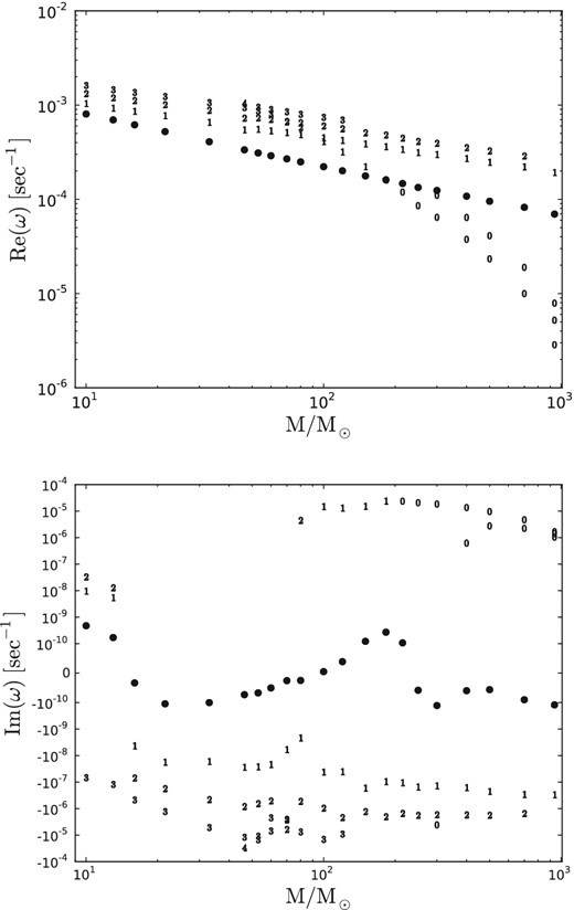
Real (first panel) and imaginary (second panel) parts of the lowest lying modes versus stellar mass. (Positive imaginary parts indicate instability.) Solid circles mark the fundamental. Other modes are marked by the number of nodes of δr/r in the core. M/M_⊙ ∈ {10, 13, 16, 21.5, 33, 46.4, 53, 60, 70, 80, 90, 100, 120, 150, 183, 200, 215, 250, 300, 400, 465, 500, 700, 983}.

Figure 7.

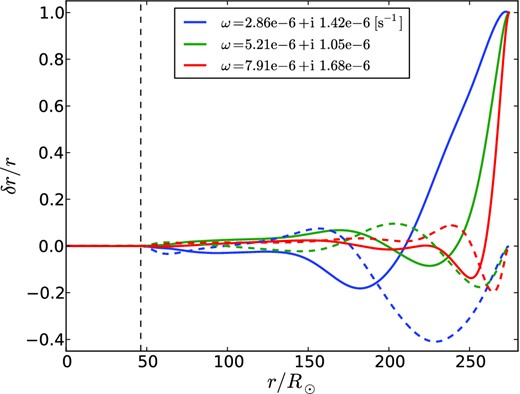
Three strange modes of the 938 M_⊙ model, with frequencies as shown. Solid and dashed curves show real and imaginary parts of the eigenfunctions, respectively. Thin vertical dashed line divides the core from the shelf (see Fig. 2). Note eigenfunctions are not weighted by r²ρ^1/2.

Our identification of the rapidly growing shelf modes with the strange modes is based largely on the variation of their eigenfrequencies with mass and the concentration of their eigenfunctions in the shelf. Papaloizou et al. (1997) propose as the definitive test of ‘strangeness’ that the modes should persist in the limit that ωt_thermal → 0. We have not made this test but note that the shelf regions of our most massive models are even more extreme than those of GK93 with respect to radiation-pressure dominance and short thermal times. We refer the reader to Papaloizou et al. (1997) and GK93 for further discussion of the linear physics of strange modes.

5 Non-linear Saturation

Appenzeller (1970) proposed that radial pulsations of very massive stars saturate in shocks that eject mass. His criterion for the onset of shocks was that the radial velocity at the photosphere becomes larger than the local sound speed. Papaloizou (1973a) found in his own numerical calculations that shocks were not so easily formed, and saturation occurred without mass loss. Our view is closer to Papaloizou's, but we emphasize coupling to non-radial modes rather than radial overtones, at least for the fundamental and other near-adiabatic modes. Saturation of strange modes is more likely to yield shocks and is discussed briefly in Section 5.2 below.

The largest growth rates we find are |${\lesssim } 10 t_\mathrm{KH}^{-1}$|⁠. Here t_KH is the Kelvin–Helmholtz time defined as by Goodman & Tan (2004), which asymptotes to t_KH ≈ 3000 yr in the limit of very large masses.² On the other hand, the pulsation periods recorded in Table 2 are ≲1 d, and we expect this to scale ∝ M^−1/2 at higher masses. Thus the growth times are on the order of 10⁵ pulsation periods. In this sense, the instabilities are extremely weak, even if the possibly stabilizing influence of convection is ignored.

At one level, this is not a surprise. Whether caused by the ϵ- or κ-mechanism, pulsational instability operates by modulating the heat content of the star on the pulsation period. Thus, the smallness of the ratio |ω_i/ω_r| reflects the disparity between the characteristic thermal and dynamical times of the star. We shall shortly argue that the smallness of the linear growth rate implies a small amplitude at non-linear saturation.

This is not inconsistent with the relatively large amplitudes of oscillation of classical Cepheids (δR/R ∼ 0.1) because the linear growth times are only ∼100 pulsation periods in those stars (e.g. Castor 1971; Bono, Marconi & Stellingwerf 1999), and it is worth recalling why (e.g. Cox & Giuli 1968). Classical Cepheids are evolved stars with degenerate cores and a very large ratio of central to mean density. Consequently, the eigenfunction ζ(r) ≡ δr/r of the fundamental radial mode is very far from homologous, |$\zeta (0)/\zeta (R) \sim \bar{\rho }/\rho (0) \ll 1$|⁠. The mode mass – the factor by which one multiplies the mean-square radial velocity at the surface to get the total energy in the mode – is many orders of magnitude smaller than the total mass of the star. In other words, for a given surface amplitude δR/R, the stored energy in the mode is much less than it would be if the pulsations were homologous, by a factor |${\propto } M_\mathrm{mode}/M_{\ast }$|⁠. Since the driving regions for the κ-mechanism lie near the surface, the work integral is insensitive to the mode mass: it is of order Π₀ δL δR/R, where δL/L ∼ δR/R ∼ −δT/T is the modulation of the surface luminosity and |$\Pi _0 \equiv 2\pi \omega _\mathrm{r}^{-1}$| is the pulsation period. Therefore the growth rate, which scales with the ratio of the work done per cycle to the stored energy in the mode, is |${\sim } (M_{\ast }/M_\mathrm{mode})t_\mathrm{KH}^{-1}$|⁠. The ϵ-mechanism is negligible in Cepheids because the nuclear-burning regions are in shell sources near the centre, where δ log T and δr/r are much smaller than in the ionization zones.

As a quantitative example, we have used mesa to create a ‘Cepheid’ with the following parameters: M_* = 5.7 M_⊙, R_* = 28.85 R_⊙, T_eff = 5900 K, and L = 906 L_⊙. For this model, |$\bar{\rho }/\rho (0) = 6.2\times 10^{-8}$|⁠, while ζ(0)/ζ(R_*) = 3.3 × 10^{− 6} and |$M_\mathrm{mode}/M_{\ast } = 8.4\times 10^{-5}$| for the fundamental radial mode computed with adipls. By contrast, for the 938 M_⊙ main-sequence model we find ζ(0)/ζ(R) = 0.66 and |$M_\mathrm{mode}/M_{\ast } = 0.061$|⁠.³

Thus the fundamental mode is approximately homologous and involves a significant fraction of the star's mass. We expect |$M_\mathrm{mode}/M_{\ast }$| to be nearly constant and comparable to this for larger masses because of the similarity of these models to isentropic n = 3, Γ₁ = 4/3 polytropes. Thus we also expect the growth rates of the fundamental radial mode to remain |${\lesssim } 10t_\mathrm{KH}^{-1}$|⁠, due to the relatively homogeneous structure and homologous pulsation of these very massive main-sequence models, regardless of the details of the excitation mechanisms and of the shelf or wind.

5.1 Saturation of the fundamental via three-mode coupling

As a general rule, instabilities with smaller linear growth rates saturate at lower amplitudes. A simple model equation for the amplitude envelope A > 0 might be

\begin{equation} \frac{\mathrm{d}A}{\mathrm{d}t} = \omega _\mathrm{i}A - \nu A^{n+1}, \end{equation}

(12)

in which ω_i is the linear growth rate, while ν and n describe the non-linearities. If ω_i, ν, and n are all positive, then equilibrium is reached at A_sat = (ω_i/ν)^1/n. As noted above, pulsations in classical Cepheids grow relatively rapidly. Saturation in these stars and in RR Lyraes occurs via shocks and non-linear modification of the conditions in the driving (ionization) zones (Christy 1966). Because of their much smaller dimensionless growth rates (ω_i/ω_r ∼ 10⁻⁶ instead of ∼10⁻³), the massive main-sequence stars considered here may saturate at lower amplitudes, where more delicate non-linearities may be effective.

Dziembowski (1982) suggested that three-mode coupling is responsible for saturation in dwarf Cepheids, and that this explains why they oscillate at lower amplitudes than do classical Cepheids. He worked directly from non-linear equations of motion. But if dissipation is weak, an action principle, which is necessarily adiabatic, can be efficient in describing mode couplings. The Lagrangian density |$\mathcal {L}(\xi ,\dot{\xi })$| is expanded in powers of the displacement |$ \xi $| and its time derivative |$\dot{\xi }$|⁠. The quadratic terms (⁠|$\mathcal {L}_2$|⁠) yield the linearized equations of motion, while cubic and higher terms (⁠|$\mathcal {L}_3+\mathcal {L}_4+\cdots$|⁠) describe non-linear couplings. When the amplitude of the primary/‘parent’ mode grows slowly from small amplitudes, the cubic non-linearities are the first to come into play. The most important couplings are those that are resonant, meaning that the linear eigenfrequencies of the parent and daughter modes satisfy ω_p ≈ ω_d1 + ω_d2, so that secular transfers of energy can occur.⁴ However, the corresponding Hamiltonian density |$\mathcal {H}_2+\mathcal {H}_3$| cannot be positive definite since the components of |$\xi$| can have either sign, so that the higher order non-linearities must dominate if the amplitudes pass some threshold, perhaps leading to shocks and a breakdown of the Lagrangian description. Actually, even when the amplitudes remain small, dissipative terms must be added to the equations of motion to describe the linear damping of the daughter modes. In application to pulsating stars, the growth rate of the parent is also represented by a non-adiabatic term. The daughter modes are usually smaller in wavelength than the parent and therefore more easily damped by radiative diffusion or (perhaps) eddy viscosity.

Landmark applications of three-mode coupling to the saturation of stellar instabilities include those by Wu & Goldreich (2001) (to white dwarf/ZZ Ceti stars), as well as Schenk et al. (2002) and Arras et al. (2003) (to rapidly rotating neutron stars). Papaloizou (1973a) argued that pulsations of very massive stars driven by the ϵ-mechanism can saturate via direct resonant couplings: that is, the coupling of a quadratic or higher power of the fundamental mode to a higher frequency radial p mode (overtone), so that nω_f ≈ ω_d for some integer n > 1. Non-radial daughter modes offer many more possibilities for resonance, however, g-modes are necessarily non-radial and have low frequencies, which is important for resonances of the type ω_p ≈ ω_d1 + ω_d2 because the frequency of the fundamental, ω_f, is somewhat lower relative to the characteristic dynamical frequency |$\omega _{\ast } \equiv (GM_{\ast }/R_{\ast }^3)^{1/2}$| than in less massive stars, the ratio |$\omega _\mathrm{f}/\omega _{\ast }$| scaling as M^−1/2 (Goodman & Tan 2004). Therefore we focus on couplings of this type. When the parent is the radial fundamental mode, the strongest three-mode couplings are usually parametric subharmonic, meaning that the two daughter modes are two copies of the same mode, with frequency ω_d ≈ ω_f/2. The eigenfunction of a typical daughter mode is high order, with many nodes in radius and angle, but its square is non-negative and hence may have a significant three-mode coupling with the nodeless radial fundamental. Parametric subharmonic destabilization of g-modes and internal waves has been studied experimentally as well as theoretically (Benielli & Sommeria 1998, and references therein).

We use our most massive (938 M_⊙) model as an example. Most of the star convects, but there is a radiative zone at 29 ≲ r/R_⊙ ≤ 41 containing 0.026M. (There is also a second radiative zone at r ≥ 44 R_⊙, and still others in the shelf, but these contain much less mass, so we neglect them here.) The peak of the Brunt–Väisälä frequency is |$N_\mathrm{max} = 2.94\omega _{\ast }$|⁠, whereas the frequency of the fundamental radial mode is |$\omega _\mathrm{f}= 1.1446\omega _{\ast } \approx 7.116\times 10^{-5}\,\mathrm{rad\,s^{-1}}$| according to adipls (which computes only the real part), in good agreement with our non-adiabatic code. Thus there are many g-modes with frequencies ∼ω_f/2. Using the approximate Wentzel–Kramers–Brillouin (WKB) dispersion for high-order g-modes,

\begin{equation} \frac{\sqrt{l(l+1)}}{\omega _{ln}} \int N(r) \frac{\mathrm{d}r}{r} \approx \pi \left(n-\frac{1}{2}\right) \end{equation}

(13)

(where n ≥ 1 counts radial nodes) and the profile of the Brunt–Väisälä frequency in the radiative zone, N(r), we estimate that n/l ≈ 0.34 for ω_ln ≈ ω_f/2 and l, n ≫ 1. For a non-rotating spherical star, so that the eigenfrequency is independent of spherical-harmonic order m, the number of mode frequencies in a given interval Δω near ω_f/2 that correspond to g-modes of degree l^′ ≤ l scales as 0.17 l²Δlog ω when l ≫ 1. Inverting this, the minimum l at which one expects to find modes in the interval Δω is

\begin{equation} l_\mathrm{min}(\Delta \omega ) \approx 2.4\left(\frac{\Delta \omega }{\omega }\right)^{-1/2}\text{.} \end{equation}

(14)

The distance Δω from exact subharmonic resonance at which daughter modes can grow depends upon the linear damping rate of these modes, the amplitude of the parent, and the three-mode coupling coefficient. For the damping time of high-order g-modes by radiative diffusion, we apply equation (4.8) of Dziembowski (1982) to our 938 M_⊙ model:

\begin{equation} t_\mathrm{damp} = \gamma _\mathrm{d}^{-1} \approx 1.0 \left(\frac{30}{l}\,\frac{\omega _\mathrm{f}}{2\omega }\right)^2\,\mathrm{yr}\text{.} \end{equation}

(15)

We evaluate the three-mode coupling coefficient from equation (A8) of Kumar & Goldreich (1989). Their formula assumes that the adiabatic exponent Γ₁ is constant and neglects the Eulerian perturbation to the gravitational potential, which, although essential for the eigenfrequency of the fundamental mode, is unimportant for the coupling since most of the stellar mass lies interior to the propagation region of the g-modes in our case. We make the further approximation that the fundamental mode is exactly homologous, meaning that its radial displacement is given by δr(r, t) = ζr cos (ω_ft), with ζ spatially constant but growing slowly as exp (ω_it). We approximate the daughter mode eigenfunctions using WKB, neglecting terms of relative order (k_rH_P)⁻¹, where |$k_r \approx \sqrt{l(l+1)}N/\omega r$| is the radial wavenumber and H_P the pressure scale height, and find that

\begin{equation} \int \mathcal {H}_3 \text{d}^3\boldsymbol {x} = \cdots + \left(\frac{3\Gamma _1-1}{2}\right) \zeta \cos \omega _\mathrm{f}t \int N^2\delta r_\mathrm{d}^2 \,\mathrm{d}M\text{.} \end{equation}

(16)

Here ‘⋅⋅⋅’ represents all three-mode coupling other than the one of interest, while δr_d = q_d(t)ξ_r,d(r)Y_lm(θ, ϕ) is the radial displacement of the daughter mode, with time-dependent amplitude q_d(t). For simplicity, we set Γ₁ = 4/3, though the mass-averaged value of Γ₁ in the 938 M_⊙ model is ≈1.37.

The integrand of equation (16) is twice the potential energy per unit mass of the g-mode. The coupling term can therefore be treated as though it were a time-dependent correction to the linear dynamics of the daughter mode, whose amplitude evolves according to

\begin{equation} \ddot{q}_\mathrm{d}+ 2\gamma _\mathrm{d}\dot{q}_\mathrm{d}+ \omega _\mathrm{d}^2 \left[1 + 3\zeta \cos (\omega _\mathrm{f}t)\right]q_\mathrm{d}= 0\text{.} \end{equation}

(17)

As usual with such Mathieu equations, if ζ and γ_d/ω_d are both small, then the solutions for q_d(t) are approximately sinusoidal but with envelopes varying as exp (st):

\begin{equation} s = -\gamma _\mathrm{d}\pm \frac{3\zeta \omega _\mathrm{d}}{4} \sqrt{1-\left(\frac{4\Delta \omega _\mathrm{d}}{3\zeta \omega _\mathrm{d}}\right)^2}, \quad \Delta \omega _\mathrm{d}\equiv \omega _\mathrm{d}- \frac{1}{2}\omega _\mathrm{f}\text{.} \end{equation}

(18)

Thus in order that the daughter mode should grow even at exact resonance (Δω_d = 0), we must have ζ > 4γ_d/3ω_d. Since γ_d ∝ l² (equation 15), this sets an upper bound to the degrees of daughter modes that can be destabilized when the amplitude of the fundamental is δR/R = ζ ≪ 1. Yet l must be large enough so that it is probable to find eigenfrequencies within the range |Δω_d| ≤ 3ζω_d/4 for which the square root in equation (17) is real. Thus in effect we must evaluate γ_d at the degree l_min that is found by setting Δlog ω ≈ ζ in equation (14). Then |$\gamma _\mathrm{d}\propto l_\mathrm{min}^2 \propto \zeta ^{-1}$|⁠, so that the requirement |$\frac{3}{4}\zeta \omega _\mathrm{d}> \gamma _\mathrm{d}$| for growth leads to an inequality of the form ζ > Cζ⁻¹. Evaluating the numerical factor C, we find that the threshold for exciting daughter modes is approximately

\begin{equation} \left(\frac{\delta R}{R}\right)_\mathrm{min} \approx 3\times 10^{-3}\text{,} \quad l_\mathrm{d}\approx 45\text{.} \end{equation}

(19)

Since the mode frequencies are sensitive to details of the stellar model, the occurrence of resonance is effectively probabilistic, and therefore the threshold for subharmonic instability will vary somewhat. In fact, for the particular model considered here, adipls finds Δω_d/ω_d ≈ 4 × 10⁻⁴ at l_d = 26, which is some 20 times closer to resonance than would be expected from the statistical estimate (14).

The threshold (19) of subharmonic instability involves only the current amplitude of the fundamental mode, not its rate of growth, ω_i. The latter is important for deciding whether the daughter modes can actually accept and dissipate energy from the parent faster than the non-adiabatic work integral increases that energy. Arras et al. (2003) state as a rule of thumb that the condition for this is simply γ_d > ω_i, a regime they call ‘weak driving’. Clearly this would suffice for non-linear saturation of the unstable parent mode if a daughter mode could reach energy equipartition with the parent, but that is unlikely in our case. The wavelength of the first daughters to go unstable is much smaller than the radius of the star, roughly by a factor 2/l when one accounts for both the radial and angular components of the wavenumber. Also the mass of the g-mode propagation zone is only 0.026M, whereas the effective mass of the fundamental mode is 0.061M, as previously discussed. Therefore if a daughter mode at, say, l_d = 45 were to have the same energy as the fundamental, it would have a strain rate (spatial derivative of velocity) roughly |$2\pi (l/2) \sqrt{0.061/0.026} \approx 5.\,l$| times larger than the parent. At such a strain rate, the daughter mode would destabilize still other modes (granddaughters) and probably transfer energy to them more quickly than it could receive energy from the parent. Therefore equipartition is unlikely.

On the other hand, γ_d ≫ ω_i in the present case, so that the rate of linear dissipation by daughter modes could balance the growth of the parent even if the daughters’ energies were well below equipartition with the parent. Because of the degeneracy of the eigenfrequencies in a non-rotating star, 2l_d + 1 daughter modes grow at the same rate. When the average energy per mode reaches a value |$\bar{E}_\mathrm{d}$|⁠, the total linear dissipation rate becomes |$2(2l_\mathrm{d}+1) \gamma _\mathrm{d}\bar{E}_\mathrm{d}$|⁠. Setting this equal to the rate at which the fundamental mode gains energy from its own linear instability, 2ω_iE_f, shows that saturation is possible when |$\bar{E}_\mathrm{d}/E_{\rm f} \approx (2l_\mathrm{d}+1)^{-1}(\omega _\mathrm{i}/\gamma _\mathrm{d})$|⁠. Evaluating this for l_d = 45, |$\gamma _\mathrm{d}^{-1} \approx 0.46\,\mathrm{yr}$| (cf. equation 15), and ω_i = (500 yr)⁻¹ leads to |$\bar{E}_\mathrm{d}/E_{\rm f} \approx 10^{-5}$|⁠. The ratio of strain rates is then

\begin{equation} \frac{1}{2}\sqrt{\frac{\bar{E}_\mathrm{d}}{E_{\rm f}}} 4.6 l_\mathrm{d}\approx 0.3 \quad (l_\mathrm{d}\approx 45) \end{equation}

(20)

(a factor of 1/2 reflects the lower frequency of the daughters). Since this is less than unity, saturation of the parent/fundamental mode is likely at daughter amplitudes too small to excite granddaughters.

We conclude that it is indeed likely that three-mode coupling will saturate the growth of the fundamental radial mode. However, some caveats are in order regarding rotation, which we have so far neglected.

There are at least two rotational regimes to consider: slow and fast. Slow rotation at an angular velocity |$\Omega \gtrsim l_\mathrm{d}^{-1}\omega _{\ast }$| but ≪N_max will lift the degeneracy with respect to spherical-harmonic order m, while preserving the degree l as a useful approximate quantum number. Since there are more distinct eigenfrequencies, subharmonic resonance becomes possible at smaller l: equation (14) is replaced by l_min ≈ 1.6(Δω/ω)^−1/3 → 0.6ζ^−1/3. Otherwise following the same steps as before, the threshold of instability occurs at ζ ≈ 5.4 × 10⁻⁴ and l_d ≈ 20 (both lower than before). Now a single, non-degenerate daughter mode first goes unstable, so the required balance at saturation if this daughter only is active becomes |$2\gamma _\mathrm{d}\bar{E}_\mathrm{d}= 2\omega _\mathrm{i}E_{\rm f}$|⁠, and the ratio of strain rates (daughter:parent) works out to ≈3 instead of 0.3. Hence non-linear coupling of the daughter to granddaughters may occur, limiting the energy of the former and complicating the analysis. On the other hand, the number of unstable daughters will increase rapidly (∝ ζ^5/2) as the amplitude of the parent increases above the first subharmonic threshold, so without having analysed the situation carefully, we still expect saturation to occur.

By fast rotation, we mean fast enough so that inertial oscillations – approximately incompressible motions restored by Coriolis rather than buoyancy forces – can have resonant three-mode couplings with the parent, as considered by Schenk et al. (2002) and Arras et al. (2003) for neutron stars. Since the maximum frequency of inertial oscillations is 2Ω, a necessary condition for subharmonic instability of the fundamental mode is Ω > ω_f/4. In the 938 M_⊙ model, this translates to Ω > 0.286ω_*, which is half or less of the mass-shedding limit for an n = 3 polytrope, depending how one defines ω_* for a non-spherical body (Hurley & Roberts 1964). Rapid rotation is not unreasonable for a body recently formed by fragmentation of an active galactic nucleus (AGN) accretion disc. Furthermore, |$\omega _\mathrm{f}/\omega _{\ast }$| scales as M^−1/2 with increasing stellar mass.⁵ Unlike g-modes, inertial oscillations propagate in convection zones, so that they may be destabilized throughout these (largely convective) massive stars. This is salient because we are not sure how the mass fraction of the radiative zones should scale at masses above 10³ M_⊙ and supersolar metallicities. Even when the condition Ω > ω_f/4 is not satisfied, the imposition of rotation on vigorous convection will surely lead to magnetic fields, perhaps in rough equipartition with the convection, so that radial pulsations may couple non-linearly to small-scale Alfvénic modes.

5.2 Saturation of strange modes

Because of their large growth rates, strange modes are unlikely to saturate via three-mode couplings of the sort discussed above. They will grow to large amplitudes and probably saturate via shocks.

As a conservative criterion for the amplitude at which a shock appears, we take |$|\mathrm{\partial} \delta r/\mathrm{\partial} r|_{\rm \max }\ge 1$|⁠, since this would predict shell crossing in the absence of shocks. For the fastest growing strange mode of the 938 M_⊙ model, |$|\mathrm{\partial} \delta r/\mathrm{\partial} r|_{\rm \max } = 25.9 \delta R/R$|⁠. The maximum is achieved at r = 0.984R. Shocks may then appear when the surface amplitude δR/R = (25.9)⁻¹ ≈ 4 per cent. At this point, the amplitude of the displacement eigenfunction at the surface of the core (r ≈ 0.169R) will be only 1.4 × 10⁻⁶. The corresponding numbers for the other two strange modes of this model are 2 × 10⁻⁶ and 7 × 10⁻⁶. Given the smallness of these numbers, it seems inconceivable that strange modes could threaten the survival of the star on dynamical time-scales.

Whether finite-amplitude strange modes drive mass loss from the shelf is a different and difficult question. On the one hand, the maximum radial velocity at shock onset is rather small (≲5 per cent) compared to the escape velocity v_esc = (2GM/R)^1/2. On the other hand, the residual between gravitational and radiative accelerations is relatively small, so that escape may be possible at v ≪ v_esc. Furthermore, line-driven steady winds are likely even without the assistance of shocks. If the mass-loss rate of such a wind is high enough, it may tend to suppress the linear instability of the strange modes. All of this we leave for later investigation.

6 SUMMARY AND DISCUSSION

We have re-examined the stability of the fundamental radial mode of very massive main-sequence stars. Although non-radial and higher order radial modes may also be unstable, we focus on the radial fundamental because collapse or explosion of these radiation-pressure-dominated objects would begin with this mode at linear order. In agreement with SQA, we find that the linear growth rate is sensitive to turbulent convective damping. We have extended their results to higher masses at solar metallicity, and we have used a fully non-adiabatic rather than quasi-adiabatic method, which allows us to treat the κ-mechanism more reliably. The ϵ-mechanism is more important for our most massive models we consider, however.

The linear growth rates remain uncertain not only because of the turbulent bulk viscosity, but also because of the tenuous (and possibly unphysical) envelopes possessed by all of our models above 100 M_⊙. In fact we find negative growth rates even without convection, apparently due to radiative damping in the shelf. Nevertheless, the growth rate should in any case be extremely small even if positive, ω_i/ω_r ∼ Π₀/t_KH, due to the relatively low central concentrations of these stars and correspondingly large mode masses.

We have then argued from the smallness of the linear growth rate (in case this is positive) that the radial fundamental should saturate at a small amplitude due to any one of a number of weak non-linearities. To support this claim, we have estimated the saturation amplitude that would result if parametric coupling to high-order g-modes were the most important non-linearity. For our most massive model, the estimate is δR/R ≈ 3 × 10⁻³. Other non-linear couplings may stop the growth at even smaller amplitudes, but those we identify would depend on uncertain parameters such as the star's rotation rate or magnetic field.

We have also shown that our models, like those of GK93, are subject to a class of intrinsically non-adiabatic modes having much larger growth rates but confined to the shelf: strange modes. These we estimate to saturate at fractional surface displacements of a few per cent via shocks. Their contribution to mass loss, if any, can be reliably estimated only in the context of a time-dependent wind model that includes a number of other non-linear effects, such as line driving. However, even at saturation, the energy of the strange modes in the stellar core is negligible, and therefore they probably affect the bulk of the star only secularly.

A number of physical simplifications and compromises have been made: restriction to solar metallicity; neglect of rotation; and neglect of perturbations to the convective flux. Increased metallicity might produce even more extended ‘shelves’ in the equilibrium models, and larger growth rates for the modes driven by the ϵ-mechanism. However, presuming that the growth rates of the fundamental mode varied roughly linearly with Z, they would remain very small compared to the dynamical time even at metallicities 10 times solar, such as may obtain in AGN discs (Dietrich et al. 2003; Nagao, Marconi & Maiolino 2006). Rotation is expected to have a stabilizing influence on the fundamental mode at very high masses because it contributes to the perturbed energy under homologous changes in radius somewhat like gas rather than radiation pressure (Baumgarte & Shapiro 1999). This could be important for very massive stars formed in an AGN disc, and perhaps continually accreting from that disc, since such objects would probably rotate rapidly (Goodman & Tan 2004; Jiang & Goodman 2011). Neglect of perturbations to the convective flux has surely caused quantitative errors in the growth rates. Guzik & Lovekin (2012), using a prescription for such perturbations that incorporates a time delay in the convective response, find that super-Eddington luminosities can occur during part of the pulsation cycle, perhaps leading to mass loss. However, their analysis is limited to the outer parts of the star. More importantly, their prescription relies on mixing-length theory, which may not be reliable in the extremely radiation-pressure-dominated shelf regions (Jiang et al. 2015).

Despite these simplifications and uncertainties, it seems likely that the growth rate of the fundamental mode must be extremely small compared to the reciprocal of the dynamical time, and therefore that pulsations in the fundamental will saturate non-linearly at small amplitudes too small to disrupt or collapse the star – at least on the main sequence. We conclude that thermally driven pulsations of the radial fundamental mode do not limit the main-sequence lifetimes of very massive stars. The tenuous outer envelopes of the more massive mesa models, however, which stem from an opacity bump at ∼10⁵ K, lead us to suspect that these stars would have powerful winds if the hydrostatic constraint were lifted, and that the mass-loss time-scale (⁠|$M_{\ast }/\dot{M}$|⁠) may be much less than 1 Myr, though necessarily longer than the Kelvin–Helmholtz time-scale (≈3000 yr). The lower bound would be achieved only if all of the stellar luminosity were converted to the mechanical energy of a wind with vanishing asymptotic velocity at infinity. For a very massive star embedded in a dense AGN disc, continued accretion from the disc might easily exceed the wind losses, perhaps causing it to grow to such a mass as to undergo relativistic instability.

These results suggest a few directions for future research. It will be relatively straightforward to explore the effect of supersolar metallicities on the linear growth rates. Changes in the growth rates as the models evolve away from the ZAMS could also be studied, although we have not yet succeeded in evolving our most massive mesa models to the end of their main-sequence phases. Probably more important, but also more challenging, will be to determine the mass-loss time-scale. Several physical mechanisms will have to be considered, including line-driven winds (Castor, Abbott & Klein 1975); inhomogeneous optically thick winds (Owocki 2015); and perhaps winds driven by non-linear strange modes or other radiation-driven instabilities. Still more mechanisms may operate in late stages of stellar evolution, such as wave-driven winds (Quataert et al. 2015). The range of possibilities is narrowed if one focuses on mechanisms that operate early in the life of a star and that are capable of removing much of its initial mass in much less than the nominal main-sequence lifetime. Even so, multidimensional calculations with frequency-dependent radiative transfer may be required.

This project made extensive use of the mesa stellar evolution code and the adipls asteroseismology package.

1

It is possible that some low-lying modes have been missed. At the higher masses, the search for modes becomes tedious, especially for the strongly non-adiabatic modes. There are several causes, but the most pernicious is that each complex zero of the objective function described in Appendix A is paired with a pole, and the separation between poles and zeros decreases with increasing mass. This makes it difficult for zero-finders to ‘smell’ their quarry from a distance in the complex plane.

2

In order that the estimate of t_KH not be biased by the extended but almost massless shelf, we use for R the radius of the base of the shelf as defined in Section 3.

3

This depends upon what one considers to be the stellar ‘surface.’ For the purpose of calculating M_mode, we use R_shelf (Section 3) when this is distinctly less than the photospheric radius.

4

In resonance conditions such as this, all frequencies are understood to be real and non-negative.

5

Uniform rotation at the mass-shedding limit may set a lower limit to |$\omega _\mathrm{f}/\omega _{\ast }$| because rotational energy behaves somewhat like gas pressure in the time-dependent virial theorem. Because of the central concentration of n = 3 polytropes, however, we estimate that this limit comes into effect only for M ≳ 10⁵ M_⊙, where relativistic corrections must also be considered (Baumgarte & Shapiro 1999).

6

The eigenvalues {λ₁, …, λ_n} of |$\bf {A}$| at a particular x should not be confused with the eigenvalue ω of the entire boundary-value problem. It might be better to speak of wavenumbers k_x ≡ −iλ. Since |$\bf {A}$| depends upon ω as well as x, the λs and k_xs do as well.

7

They satisfy − iωδT ≈ η∂²δT/∂r², where |$\eta =16\sigma _{\small {sb}}T^3/3\kappa \rho ^2 c_P$| is the thermal diffusivity. Hence the eigenvalues |${\rm i}k_r\approx \pm \sqrt{-{\rm i}\omega /\eta }$|⁠.

REFERENCES

Appenzeller

I.

1970

A&A

9

216

Arras

P.

Flanagan

E. E.

Morsink

S. M.

Schenk

A. K.

Teukolsky

S. A.

Wasserman

I.

2003

ApJ

591

1129

Baumgarte

T. W.

Shapiro

S. L.

1999

ApJ

526

941

Benielli

D.

Sommeria

J.

1998

J. Fluid Mech.

374

117

Bonanos

A. Z.

et al.

2004

ApJ

611

L33

Bono

G.

Marconi

M.

Stellingwerf

R. F.

1999

ApJS

122

167

Brickhill

A. J.

1991

MNRAS

251

673

Castor

J. I.

1971

ApJ

166

109

Castor

J. I.

Abbott

D. C.

Klein

R. I.

1975

ApJ

195

157

Chandrasekhar

S.

1964

ApJ

140

417

Christensen-Dalsgaard

J.

2008

Ap&SS

316

113

Christy

R. F.

1966

ApJ

144

108

Cox

J. P.

1980

Theory of Stellar Pulsation

Princeton Univ. Press

Princeton, NJ

Cox

J. P.

Giuli

R. T.

1968

Principles of Stellar Structure

Gordon & Breach

New York

Crowther

P. A.

Schnurr

O.

Hirschi

R.

Yusof

N.

Parker

R. J.

Goodwin

S. P.

Kassim

H. A.

2010

MNRAS

408

731

Davey

A.

1983

J. Comput. Phys.

51

343

Dhanda Batra

N.

Baldwin

J. A.

2014

MNRAS

439

771

Dietrich

M.

Hamann

F.

Shields

J. C.

Constantin

A.

Heidt

J.

Jäger

K.

Vestergaard

M.

Wagner

S. J.

2003

ApJ

589

722

Drury

L. O.

1980

J. Comput. Phys.

37

133

Dziembowski

W.

1982

Acta Astron.

32

147

Figer

D. F.

2005

Nature

434

192

PubMed

Glatzel

W.

Kiriakidis

M.

1993

MNRAS

262

85

(GK93)

Goodman

J.

Tan

J. C.

2004

ApJ

608

108

Gräfener

G.

Owocki

S. P.

Vink

J. S.

2012

A&A

538

A40

Grevesse

N.

Noels

A.

1993

Phys. Scr. T

T47

133

Guzik

J. A.

Lovekin

C. C.

2012

Astron. Rev.

7

13

Hamann

F.

Ferland

G.

1999

ARA&A

37

487

Henyey

L.

Vardya

M. S.

Bodenheimer

P.

1965

ApJ

142

841

Hurley

M.

Roberts

P. H.

1964

ApJ

140

583

Iglesias

C. A.

Rogers

F. J.

1996

ApJ

464

943

Jiang

Y.-F.

Goodman

J.

2011

ApJ

730

45

Jiang

Y.-F.

Cantiello

M.

Bildsten

L.

Quataert

E.

Blaes

O.

2015

ApJ

813

74

Koen

C.

2006

MNRAS

365

590

Kumar

P.

Goldreich

P.

1989

ApJ

342

558

Matsuoka

K.

Nagao

T.

Marconi

A.

Maiolino

R.

Taniguchi

Y.

2011

A&A

527

A100

Montero

P. J.

Janka

H.-T.

Müller

E.

2012

ApJ

749

37

Nagao

T.

Marconi

A.

Maiolino

R.

2006

A&A

447

157

Oey

M. S.

Clarke

C. J.

2005

ApJ

620

L43

Owocki

S. P.

Vink

J. S.

2015

Astrophysics and Space Science Library, Vol. 412, Very Massive Stars in the Local Universe

Springer-Verlag

Switzerland

113

Papaloizou

J. C. B.

1973a

MNRAS

162

143

Papaloizou

J. C. B.

1973b

MNRAS

162

169

Papaloizou

J. C. B.

Alberts

F.

Pringle

J. E.

Savonije

G. J.

1997

MNRAS

284

821

Paxton

B.

Bildsten

L.

Dotter

A.

Herwig

F.

Lesaffre

P.

Timmes

F.

2011

ApJS

192

3

Paxton

B.

et al.

2013

ApJS

208

4

Quataert

E.

Fernandez

R.

Kasen

D.

Klion

H.

Paxton

B.

2015

preprint (arXiv e-prints)

Rauw

G.

et al.

2004

A&A

420

L9

Schenk

A. K.

Arras

P.

Flanagan

É. É.

Teukolsky

S. A.

Wasserman

I.

2002

Phys. Rev. D

65

024001

Schnurr

O.

Drissen

L.

Rubert

C.

St-Louis

N.

Moffat

A. F. J.

2012

ASP Conf. Ser. Vol. 465, Proceedings of a Scientific Meeting in Honor of Anthony F. J. Moffat

Astron. Soc. Pac.

San Francisco

187

Schwarzschild

M.

Härm

R.

1959

ApJ

129

637

Shiode

J. H.

Quataert

E.

Arras

P.

2012

MNRAS

423

3397

(SQA)

Weidner

C.

Kroupa

P.

2004

MNRAS

348

187

Wu

Y.

Goldreich

P.

2001

ApJ

546

469

Zeldovich

Y. B.

Novikov

I. D.

1971

Relativistic Astrophysics. Vol. 1, Stars and Relativity

University of Chicago Press

Chicago

APPENDIX A: METHOD FOR STIFF LINEAR BOUNDARY-VALUE PROBLEMS

The method described here is similar to that of Drury (1980) and Davey (1983), but different in detail and slightly simpler, at least in derivation. One wants to solve

\begin{equation} \frac{\mathrm{d}\boldsymbol {y}}{\mathrm{d}x} = \bf {A}\boldsymbol {y}, \end{equation}

(A1)

|$\boldsymbol {y}$| being a column vector of length n representing the dependent variables, and |$\bf {A}$| an n × n matrix depending upon an eigenvalue to be determined, and usually also on the independent variable, x. In our case n = 4, and the eigenvalue is the complex frequency of pulsation, ω. There are p homogeneous boundary conditions to be satisfied at the left-hand boundary, x = x_min, and n − p at the right-hand boundary, x = x_max. These are represented by p × n and (n − p) × n matrices |$\bf {B}(x_{\min })$| and |$\bf {C}(x_{\max })$|⁠:

\begin{equation} \bf {B}(x_{\min })\boldsymbol {y}(x_{\min }) = 0,\qquad \bf {C}(x_{\max })\boldsymbol {y}(x_{\max }) = 0. \end{equation}

(A2)

One expects non-zero solutions for |$\boldsymbol {y}(x)$| only for discrete values of ω, which are to be determined.

The difficulty in solving this boundary-value problem is that the n complex eigenvalues of |$\bf {A}(x,\omega )$| may differ widely in size (Fig. A1). In our problem, they vary over 4–6 orders of magnitude in the inner parts of the star, due to the large ratio of thermal to dynamical time.⁶ Furthermore, since the eigenfunction corresponding to λ behaves as ∼exp (∫^xλdx), direct integration of equation (A1) can overflow or underflow machine precision if the real part of λ is large. This happens in our stellar problem, and both signs of Real(λ) occur simultaneously. It therefore proves impractical to use a conventional shooting method in which one iteratively makes guesses for the unconstrained components of |$\boldsymbol {y}$| at both boundaries (and for ω) and integrates towards a fitting point. As described above, a relaxation (Henyey-type) method also failed.

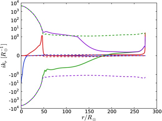
$Real (solid) and imaginary (dashed) parts of the four eigenvalues of $\bf {A}$ in the 938 M⊙ model. Vertical scale is linear within the interval $(-{\rm R}_{\odot }^{-1},\ {\rm R}_{\odot }^{-1})$, and logarithmic outside it.$

Figure A1.

Real (solid) and imaginary (dashed) parts of the four eigenvalues of |$\bf {A}$| in the 938 M_⊙ model. Vertical scale is linear within the interval |$(-{\rm R}_{\odot }^{-1},\ {\rm R}_{\odot }^{-1})$|⁠, and logarithmic outside it.