


Abstract
The relationship between stellar populations and the ionizing flux with which they irradiate their surroundings has profound implications for the evolution of the intergalactic medium (IGM). We quantify the ionizing flux arising from synthetic stellar populations which incorporate the evolution of interacting binary stars. We determine that these show ionizing flux boosted by 60 per cent at 0.05 ≤ Z ≤ 0.3 Z⊙ and a more modest 10–20 per cent at near-solar metallicities relative to star-forming populations in which stars evolve in isolation. The relation of ionizing flux to observables such as 1500 Å continuum and ultraviolet spectral slope is sensitive to attributes of the stellar population including age, star formation history and initial mass function (IMF). For a galaxy forming 1 M⊙ yr−1, observed at >100 Myr after the onset of star formation, we predict a production rate of photons capable of ionizing hydrogen, Nion = 1.4 × 1053 s−1 at Z = Z⊙ and 3.5 × 1053 s−1 at 0.1 Z⊙, assuming a Salpeter-like IMF. We evaluate the impact of these issues on the ionization of the IGM, finding that the known galaxy populations can maintain the ionization state of the Universe back to z ∼ 9, assuming that their luminosity functions continue to MUV = −10, and that constraints on the IGM at z ∼ 2–5 can be satisfied with modest Lyman-continuum photon escape fractions of 4–24 per cent depending on assumed metallicity.
1 INTRODUCTION
The epoch of reionization, during which the cold neutral intergalactic medium (IGM) of the cosmic dark ages was photoionized by the flux from the earliest luminous sources, is growing ever more accessible to observation. Colour-selected galaxy samples now include candidate galaxies at z ∼ 10 (Ellis et al. 2013; Bouwens et al. 2015), with rare spectroscopically confirmed examples out to z = 7.7 (Oesch et al. 2015). A small but growing number of quasar host galaxies are also known at z > 7 (Mortlock et al. 2011) while gamma-ray bursts have been identified at z > 8, and their host galaxies constrained (Tanvir et al. 2009, 2012; Berger et al. 2014). Observations both of the galaxy population and the IGM probed along sightlines to these distant ‘lighthouses’ have suggested that the number density of neutral hydrogen clouds rises sharply at z > 6, resulting in absorption in distant spectra, and so fewer galaxies observable in the Lyman α transition of hydrogen (Stark et al. 2010; Caruana et al. 2014; Mesinger et al. 2015). Meanwhile, increasingly precise measurements of the cosmic microwave background radiation have measured the extent to which it has been modified by neutral hydrogen along the line of sight, constraining the Thompson optical depth to reionization to τ = 0.066 ± 0.016 (Planck Collaboration XIII 2015). If interpreted as arising from a step-wise transition from neutral to ionized IGM, this corresponds to a reionization redshift of |$z=8.8^{+1.7}_{-1.4}$|. Together, these constraints suggest a reionization process that probably began around z = 10 and proceeded rapidly, leading to a Universe with a mean neutral fraction X < 1 per cent by z = 6 (Fan, Carilli & Keating 2006; Robertson et al. 2015).
Given these constraints on the history of reionization, an inevitable question arises concerning its driving force. The contribution of ionizing photons from AGN is too small to either reionize the Universe or maintain that state against hydrogen recombination, and thus star-forming galaxies are believed to power the process (Fan et al. 2006, and references therein). However, the number density of observable star-forming galaxies in the distant Universe falls sharply with cosmic time. Extrapolating the observed luminosity distribution of colour-selected, ultraviolet-luminous galaxies to below observable limits, it has been established that this population is likely sufficient to reionize the Universe but only marginally so (Robertson et al. 2015). Difficulties remain; it is unclear whether a sufficient fraction of ionizing photons are capable of escaping the dust and nebular gas within the galaxy in which they are emitted, or whether a sufficient number of small galaxies (predicted from the faint-end slope of observed luminosity functions, e.g. Bouwens et al. 2015, and poorly constrained at z > 7) exist to power cosmic reionization.
One reason for such uncertainty is the unfortunate necessity of extrapolation below the limits of observational data. Only a few, rare z > 5 galaxies are bright enough for detailed spectroscopic analysis. Observations of high-redshift galaxies are typically limited to their broad-band colours in the rest-frame ultraviolet (and sometimes optical) and perhaps a measurement of particularly strong emission lines (such as Lyman α at 1216 Å; e.g. Labbé et al. 2013; Caruana et al. 2014; Oesch et al. 2015; Smit et al. 2015). Given a measured rest-frame 1500 Å flux continuum density, usually derived from photometry in a broad bandpass, the number of ionizing photons shortwards of 912 Å (the ionization limit of hydrogen or ‘Lyman break’) must be inferred (e.g. Madau, Haardt & Rees 1999; Bunker et al. 2004; Robertson et al. 2015). This ‘Lyman-continuum’ flux is estimated through the use of stellar population synthesis models, fitted to the available data. For a stellar population of known age, metallicity and ultraviolet flux, the ionizing photon flux can be reliably estimated. However, difficulties arise when any of these properties are unknown. A young starburst will contain a larger proportion of hot, massive stars than an older one and so emit more ionizing photons for a given 1500 Å continuum measurement. By contrast, a stellar population that has formed stars continuously over its lifetime will show an ultraviolet spectral energy distribution (SED) to which both young stars and older sources contribute, resulting in a modified but far more stable ionizing photon-to-continuum ratio. At low metallicities, different stellar evolution pathways, including those which result from binary star interactions or rotation, become increasingly important — again resulting in a modified ionizing photon output (Eldridge, Izzard & Tout 2008; Stanway et al. 2014; Zhang et al. 2013; Topping & Schull 2015). While some of these variations can be inferred from stellar population modelling, this has traditionally been tuned to match the properties of the local galaxy distribution – largely comprising mature galaxies and stellar populations with a near-solar average metallicity.
As discussed in Eldridge & Stanway (2012), the general effect of binary evolution and rotation is to cause a population of stars to appear bluer at an older age than predicted by single-star models. This increase in the lifetime over which star-forming galaxies emit hard ultraviolet spectra may well present an explanation for the observed high [O iii]/H β emission line ratios in the sub-solar, low-mass star-forming galaxies of the distant Universe (Stanway et al. 2014), although the evidence for these at intermediate redshifts (z ∼ 2–3) and whether instead they may represent a shift in nitrogen abundance is still under discussion (e.g. see Sanders et al. 2015b, and references therein). Its significance for the epoch of reionization is obvious: a blue spectrum will emit more ionizing photons for a given 1500 Å luminosity than a corresponding red spectrum. Since 1500 Å (rest frame) observations, modified by a model-derived flux ratio, are most frequently used to constrain the ionizing population, it is thus critical to examine the effects of evolutionary pathways on derived constraints on reionization.
In this paper, we consider uncertainties in stellar evolution and population synthesis and how these affect the predicted ionizing flux from distant star-forming galaxies, and the interpretation of the observed galaxy luminosity function, in the context of observational constraints. In Section 2, we present the detailed theoretical stellar population models used for our analysis, and in Section 3 we explore their behaviour as a function of metallicity, age and other stellar properties. In Section 4, we predict the behaviour of key observables used to constrain the distant galaxy population, while in Section 5 we consider the implications for reionization in the context of existing measurements.
Throughout, we calculate physical quantities assuming a standard Λ cold dark matter cosmology with H0 = 70 km s−1 Mpc−1, |$\Omega _\Lambda =0.7$| and ΩM = 0.3. All magnitudes are quoted on the AB system.
2 STELLAR POPULATION MODELS
2.1 The need for stellar population models
Population and spectral synthesis codes are commonly used in astrophysics when a model for a stellar population is required. These combine theoretical (atmosphere and evolution) models or empirical spectra of individual stars, assuming some initial mass function (IMF) and stellar population age, and process the resultant emission through dust and gas screens to calculate an ‘observed’ spectrum (Leitherer et al. 1999, 2014). It is important not to overlook the assumptions that go into these models. A comprehensive analysis of some of the uncertainties in population synthesis reveals there is still much to improve in population synthesis (Conroy 2013, and references therein), refining models to address a number of physical processes that are currently not included. As Leitherer & Ekström (2012) discuss, population synthesis is currently a subject in a state of flux. Not only are the stellar atmosphere models being revised to better match the spectra of observed stars across a broad range of metallicities, stellar evolution models are also undergoing an unprecedented increase in accuracy (see e.g. Langer 2012).
Factors that affect the output of population synthesis include the effects of mass-loss rates, stellar rotation (e.g. Topping & Schull 2015) and interacting binaries (e.g. Belkus et al. 2003; Eldridge et al. 2008) which must be evaluated using detailed modelling of stellar evolution, and which are affected in turn by the IMF and metallicity of the input stellar population. Each of the widely used, publically available population synthesis codes, which include starburst99 (Leitherer et al. 1999) and Binary Population and Spectral Synthesis (bpass; Eldridge & Stanway 2012, see below) treats the above factors in a different way. An investigation of alternate implementations, stellar population assumptions and their effects is thus warranted.
2.2 Binary Population and Spectral Synthesis (BPASS)
The bpassmodels1 are a set of publically available stellar population synthesis models which are constructed by combining stellar evolution models with synthetic stellar spectra. Detailed stellar evolution models, described in Eldridge et al. (in preparation) and Eldridge et al. (2008), are combined with the latest stellar atmosphere models and a synthetic stellar population generated according to both an IMF and a distribution of binary separation distances, to produce a stellar population (see Eldridge & Stanway 2009, 2012). At solar metallicities, for mature stellar populations, a standard Salpeter (1955) IMF, and when only single-star evolution pathways are considered, the resultant output spectra are very similar to those of the well-known starburst99 code, as Fig. 1 demonstrates. At differing metallicities and ages, for different IMFs and when binary evolution pathways are included, the treatment of stellar population effects in the two codes, and hence the composite spectra they produce, diverge.
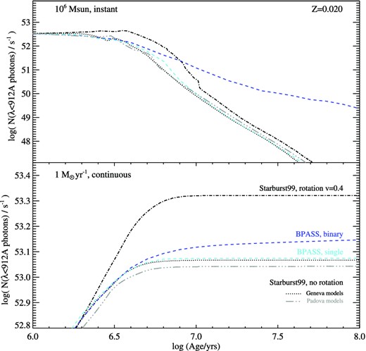
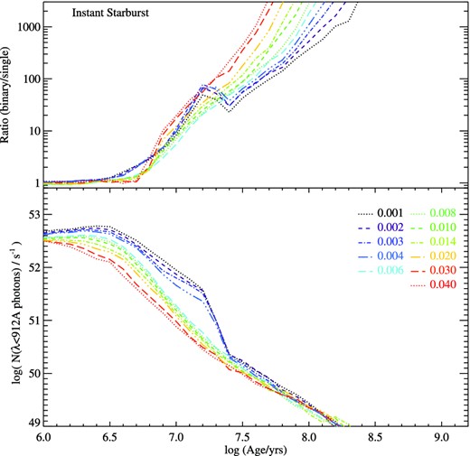
The ionizing flux generated as a function of age by synthetic stellar populations constructed using bpass with single or binary evolutionary pathways, and also by the widely used starburst99 code, forming 1 M⊙ yr−1 at near-solar metallicity. We also show an evolutionary track constructed using starburst99 and either the original Padova stellar tracks or the recent Geneva-group stellar models, a subset of which incorporate stars with a rotation parameter v = 0.4.
Interacting binaries provide a more moderate increase in ionizing flux but also reduce the rate at which it decreases in older stellar populations (see e.g. Stanway et al. 2014; Zhang et al. 2013). The three key effects of binary interactions are: removal of the hydrogen envelope in primary stars – forming more hot helium or Wolf–Rayet stars; the transfer of mass to secondary stars increasing their mass and rejuvenating them; and finally the generation of massive stars from stellar mergers (Eldridge et al. 2008). The first of these, enhanced mass loss for the primary stars in binaries, does little to increase the total ionizing flux but does allow harder ionizing photons to exist at later times than expected from a single-star population, beyond ∼10 Myr. The transfer of mass to secondary stars and binary mergers result in a more top-heavy effective mass function for the stellar population, as well as creating more massive stars at later ages than would be expected for a single-star population. These are the major reasons for the enhanced ionizing flux at late times seen for binaries in Fig. 1, and causes the slower decline rate for the ionizing flux beyond a few Myr.
Fig. 1 also illustrates the effect of stellar rotation on the predicted ionizing fluxes. Rotation tends to increase the flux at all ages but the form of evolution with stellar population age remains the same as in the non-rotating case. This is because the primary effects of rotation are to extend main-sequence lifetimes and also to generate stars that are more luminous and hotter during their main-sequence evolution.
When mass is transferred in a binary system, so too is angular momentum. This spin-up of stars by this transfer can result in the rotational mixing of its layers, allowing the more efficient burning of hydrogen in its interior (Cantiello et al. 2007; de Mink et al. 2013). At solar metallicity this can mix fresh hydrogen into main-sequence stars and rejuvenation of their age. However stellar winds are strong in such stars and so they quickly spin-down. As stellar winds weaken at lower metallicities, the stars can remain rapidly rotating over their entire main-sequence lifetimes and evolve as if they are fully mixed. This quasi-homogeneous evolution (QHE) is significant at high stellar masses ( ≳ 20 M⊙) and low metallicities (Z ≤ 0.004; see e.g. Vanbeveren, van Bever & De Donder 1997; Eldridge, Langer & Tout 2011). We have investigated the effect of QHE on stellar populations and the production of long gamma-ray bursts in Eldridge et al. (2011) and Eldridge & Stanway (2012). Others have also investigated the importance of QHE (Topping & Schull 2015) in stellar populations. This extends the stellar lifetime and causes the star to become hotter as it evolves rather than cooler (Yoon & Langer 2005).
In our fiducial population of the entire populations only approximately 0.04 per cent of the stars experience QHE. The fraction of rotationally mixed stars increases at high masses, ranging from 10 to 20 per cent of the stars above 20 M⊙. As discussed in the above papers, we have constrained the number of QHE-affected stars by ensuring that the relative rates of type Ib/c (hydrogen-free) to type II (hydrogen-rich) supernovae reproduces the observed trend with metallicity. When the first supernova occurs in a binary we calculate whether the system is disrupted or not as discussed in Eldridge et al. (2008, 2011). If the system is unbound, the secondary continues its evolution as a single star; otherwise, the remnant mass is estimated and the evolution continues with either a white dwarf, neutron star or black hole as a companion. Again mass transfer can occur but any possible luminous variability from the compact object accreting mass is not currently included. We find that only approximately 25 per cent of binary systems survive the first supernova.
The models in use here comprise version 2.0 of the bpass model data set. We employ stellar evolution and atmosphere models with a metallicity mass fraction ranging from Z = 0.001 to 0.040. These metallicities correspond to oxygen abundances spanning log(O/H)+12=7.6 to 9.0, where Z = 0.020 (log(O/H)+12=8.8) is conventionally assumed to be the value for the present-day cosmic abundance of local Galactic massive stars as discussed by Nieva & Przybilla (2012). This is preferable to using the solar composition of Asplund et al. (2009) which is closer to a log(O/H)+12=8.7 or Z = 0.014. This is because the Sun with a 4.5 billion-year age is a poor indicator for the composition of massive stars that formed much more recently. A broken power law is used for the IMF in our standard models, with a slope of −1.3 between 0.1 and 0.5 M⊙ and −2.35 at masses above this, extending to 100 M⊙ for the models used in this study. The shallow slope below a stellar mass of 0.5 M⊙ biases our models towards the more massive stellar population, and is now routinely adopted in stellar population synthesis models including the default parameters for Starburst99. The slope above the break and upper mass limit match those of the Salpeter IMF. We note that recent observations have provided evidence for stellar masses above 100 M⊙ in nearby clusters (Crowther et al. 2010), and we consider the effects of extending the IMF to higher limits in Section 3.4.
We assume an initial parameter distribution for the binary population that is flat in the logarithm of the period from 1 to 10 000 d. We also assume a flat distribution in binary mass ratio, defined as M2/M1. Both of these are consistent with the observations of Sana et al. (2012). We compute binary evolution models from 0.1 to 100 M⊙ however we only count the mass of the secondary as a star if its initial mass is greater than 0.1 M⊙, otherwise it is considered a brown dwarf and does not contribute to the total stellar mass. This assumed initial distribution leads to approximately two thirds of binary systems interacting in some way during their lifetime. We follow mass transfer between the primary to the second star, assuming that the secondary star can only accrete at a rate limited by its thermal time-scale. The remaining mass is lost from the system. We also account for QHE in the method outlined in Eldridge et al. (2011). If a secondary star accretes more than 5 per cent of its original mass then we assume it is rejuvenated and restart its evolution at its final mass at a later time. If the metallicity is Z ≤ 0.004 and the star is more massive than 20 M⊙ then we assume it evolves full mixed during its hydrogen burning lifetime and experiences QHE. While there are many uncertainty parameters in binary stellar evolution, as discussed in our previous work and the extensive literature on this topic, we do not vary these to achieve a better fit to data but work with a fiducial parameter set. These lead to a synthetic binary population that reproduces most observational tests for a stellar population and are described in detail in Eldridge et al. (2008, 2011) and Eldridge & Stanway (2009, 2012). The comparison of the V2.0 models against the same observational data will be presented in Eldridge et al. (in preparation). In total each metallicity synthetic stellar population is based on between 15 000 and 19 000 individual detailed stellar evolution models using the Cambridge STARS evolution code outlined in Eldridge et al. (2008). Stellar atmosphere models are selected from the BaSeL v3.1 library (Westera et al. 2002), supplemented by O star models generated using the WM Basic code (Smith, Norris & Crowther 2002) and Wolf–Rayet stellar atmosphere models from the Potsdam PoWR group2 (Hamann & Gräfener 2003) where appropriate.
The baseline models track the evolution of a coeval stellar population (as discussed in the next section), but can be combined to evaluate the effect of continuous star formation, multiple star formation epochs, or a more complex star formation history (see Section 3.2). They comprise both a model set with a binary distribution matching observational constraints as described above, and a single-star model set in which the stars evolve in isolation, with mass loss via stellar winds. Changes in the fraction of binary interactions can be accommodated by producing a weighted mean of these models if required.
3 EFFECTS OF STELLAR POPULATION UNCERTAINTIES
3.1 Ionizing photon output from binary populations
The key parameter required for calculations of the reionization process is, in principle, a simple one: the flux of photons with sufficient energy to ionize hydrogen (i.e. with wavelengths λ < 912 Å, a spectral region known as the Lyman continuum) arising from a stellar population. This quantity is usually estimated for a given stellar population simply from its continuum luminosity density in the far-ultraviolet, at around λ = 1500 Å in the galaxy rest frame.
In Fig. 2, we illustrate the difficulty with this characterization. We show a range of models normalized to the same far-ultraviolet luminosity, and each at the same metallicity (Z = 0.002 = 0.1 Z⊙). We adopt this as representative as it reproduces the moderately sub-solar, but non-negligible, metallicities inferred for the high-redshift (z ∼ 2–7) galaxy population (Dunlop et al. 2013; Cucchiara et al. 2015; Sanders et al. 2015a), and we defer discussion of metallicity effects to Section 3.3.
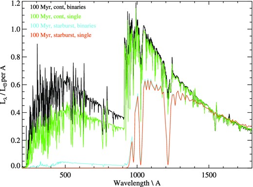
The rest-frame ultraviolet spectral region for different stellar population models with an identical luminosity at 1500 Å. Binary population synthesis models are compared to single-star models, for either an instantaneous starburst or continuous star formation rate of 1 M⊙ yr−1, at age of 100 Myr. The stellar mass of the continuous starburst models is 106.0 M⊙, while that of the starbursts is 106.9 M⊙. A stellar metallicity of Z = 0.002 is shown.
In each case the same far-ultraviolet luminosity is generated by stellar populations with similar total stellar mass, but the flux shortwards of the Lyman break at 912 Å differs significantly. Populations which incorporate binary interactions systematically generate more ionizing photons than single-star populations with the same 1500 Å continuum.
3.2 Star formation history and age
The Lyman-continuum flux for a population with continuous star formation rate 1 M⊙ yr−1 is dominated by massive stars with lifetimes of a few Myr (where 1 Myr = 106 yr). In Fig. 3, we show evolutionary tracks in ionizing photon flux and far-ultraviolet luminosity arising from a galaxy with Z = 0.002. For stellar population forming stars as a constant rate, the photon flux remains virtually constant at ages above ∼10 Myr in both the single and binary star evolution path cases as the oldest stars fade in the ultraviolet and are replaced. Throughout the lifetime of the star formation event, however, the binary star populations produce a higher number of ionizing photons, exceeding the single-star population flux by 50–60 per cent in this Z = 0.002 example (see Section 3.3 for metallicity effects).
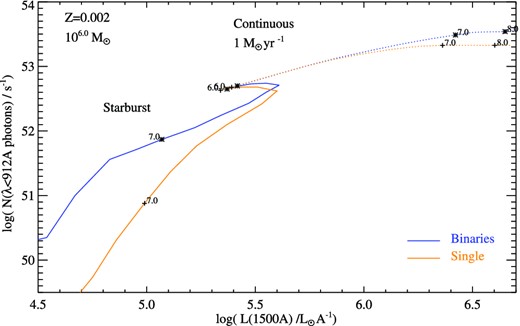
The change in ionizing photon flux over the evolution of single and binary stellar populations at Z = 0.002, for both star formation histories considered in Section 3. In the case of an ageing instantaneous starburst (solid lines), a stellar mass of 106 M⊙ is created and then allowed to age. In the case of continuous star formation (dotted line) stars are continuously added at 1 M⊙ yr−1 such that the stellar mass is equal to the stellar popular age. The logarithm of the age is indicated at labelled points. The stellar masses are identical at 106 yr after the onset of star formation.
While the continuous star formation case yields a highly stable photon flux that depends only on star formation rate (after an initial establishment period) rather than stellar mass, it may not be a wholly realistic scenario for all distant galaxies. For galaxies in which star formation is triggered by merger events, or the sudden accretion of gas clouds from the IGM, which drive winds which quench their own star formation, or which have a small gas supply at the onset of star formation, star formation could plausibly be a short-lived phase (see Bouwens et al. 2010; Verma et al. 2007). The star formation history in such systems is usually parametrized as an initial abrupt star formation event, followed by ongoing star formation, the rate of which declines exponentially with a characteristic time-scale, τ. The continuous star formation scenario represents one extreme of such models (τ = ∞), while the other extreme (τ = 0) is an instantaneous starburst, in which all stars are formed simultaneously and thereafter evolve without further star formation.
In Fig. 2, we show a comparison between the synthetic spectra produced by continuous star formation and a starburst scenario at a stellar population age of 100 Myr, using either single or binary synthesis at Z = 0.002. By contrast with the continuous star formation event, an ageing starburst emits very few ionizing photons, despite a still healthy 1500 Å continuum. This is significant for the inferences drawn from the high-redshift galaxy population. Galaxies at z > 4 are typically only detected longwards of the 1216 Å Lyman α feature, and their luminosities are measured around 1500 Å in the rest frame. As Fig. 2 demonstrates, for a young starburst, this can lead to substantial ambiguity in the estimated 912 Å and ionizing photon flux.
A suggestion that starburst events at high redshift might be short lived can be found in the very high specific star formation rates (sSFRs) of Lyman break galaxies at high redshift. Such systems, observed at z ∼ 7, can form their current stellar mass in as little as 100 Myr, assuming constant star formation at the observed rate (i.e. sSFR∼9.7 Gyr−1; Stark et al. 2013). The contribution of these short-lived bursts to the ionizing flux has largely been ignored in the past, on the basis that single-star models in particular show a rapid decline in luminosity within 10 Myr of the initial burst. In Fig. 3, we show the evolution of the photon flux with stellar population age for an instantaneous starburst. In the case of an ageing instantaneous starburst, a stellar mass of 106 M⊙ is created and then allowed to age. In the continuous star formation case, stars are continuously added to the model, weighted by IMF and at a rate of 1 M⊙ yr−1 such that the stellar mass is equal to the stellar population age. Both single-star and binary evolution synthesis models do indeed show rapid, order of magnitude, drop in ionizing photon flux over the first 10 Myr after star formation. Thereafter, however, the two populations diverge. The binary models prolong the period over which hot stars dominate the spectrum. As a result, the ionizing photon flux declines far less rapidly for binary synthesis models than that of a single-star population at the same metallicity, and the ratio between the two rises to a factor of 100 at an age of 30 Myr. The ionizing flux from these sources represents a potentially overlooked contribution to the ionizing flux in the distant Universe.
However, we note that the situations shown in Fig. 3 represent just two snapshots in a rather large parameter space. Both ionizing flux and continuum flux density will scale with star formation rate in the continuous star formation case. The same parameters will scale with mass of the initial starburst in the instantaneous case. Given a far-ultraviolet luminosity density of 106 L⊙ Å−1, we might estimate that we have a ∼100 Myr old stellar population forming 1 M⊙ yr−1, or a massive instantaneous burst (perhaps a galaxy-wide starburst due to merger activity) of the same total mass, seen at just ∼20 Myr. If the latter is in fact a better description, the ionizing photon flux is likely to be lower by an order of magnitude (assuming binary evolution, 2 orders of magnitude for single stars). More complex star formation histories, such as declining exponential starbursts, will lie between these extremes, with a strong dependence on their characteristic time-scales.
3.3 Metallicity
In Figs 4 and 5, we show the effect of metallicity on the ionizing photon production rate as a function of age for the two star formation histories discussed above. As expected, binary stellar evolution models produce a higher ionizing flux at all times and metallicities, except within 10 Myr of the onset of star formation in the case of high metallicities. The photon production rate itself shows a clear trend with metallicity in a mature (>10 Myr) continuous starburst, with the lowest metallicities considered here (one twentieth of solar) yielding the highest the photon fluxes and the most metal-rich (twice solar) yielding the lowest for a given star formation rate. The binary and single-star model populations diverge most significantly at the lowest metallicities, where the binary population produces ∼60 per cent more ionizing photons than a single-star population, and least at the highest metallicities where the predictions for continuously star-forming populations vary only ∼20 per cent between single-star and binary models.
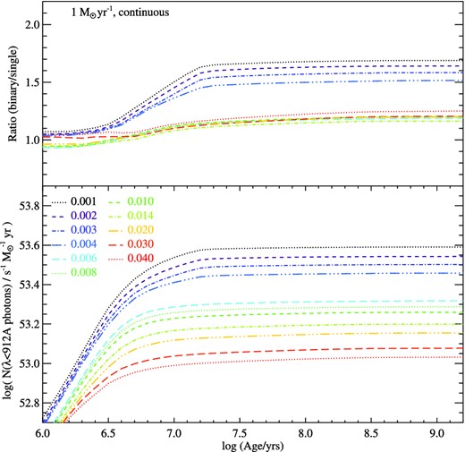
The ionizing photon flux for single and binary stellar populations with a continuous star formation rate of 1 M⊙ yr−1, as a function of age and metallicity. The upper panel shows the ratio between the two stellar evolution model sets. In both cases, the ionizing photon flux takes ∼10 Myr to establish, and thereafter remains constant, with binary evolution models predicting ∼60 per cent more ionizing photons at low metallicities, but a more modest 20 per cent at significantly sub-solar metallicities.
As in Fig. 4, for the case of an ageing instantaneous starburst with a stellar mass of 106 M⊙.
This behaviour with metallicity arises partly from an effect that can be seen in the instantaneous starburst evolution shown in Fig. 5. At metallicities below a few tenths of solar, binary evolution pathways extend the period over which a starburst shows high ionizing flux levels (within 2 orders of magnitude of the zero-age stellar population), from a few million years up to ∼20 Myr. By contrast, higher metallicity models show a rapid decline in the ionizing flux from an ageing stellar population, as processes such as QHE (due to rotation) are unable to operate effectively. The result is that in composite populations, at low-to-moderate metallicities, there are a large number of ultraviolet-luminous stars in the 10-20 Myr age range that contribute to binary, but not to single-star, models. This leads to fluxes 1–2 orders of magnitude higher in binary populations at a time immediately after the death of the most massive (and therefore ionizing) stars in the single-star models.
The metallicity dependence of the steady-state photon flux, seen at 100 Myr after the onset of continuous (1 M⊙ yr−1) star formation, is shown in Fig. 6. The variation between our lowest and highest metallicity models is a factor of almost four in ionizing photon flux. As can be seen, there is a strong trend with metallicity, with metal-poor photons producing a higher ionizing photon flux, at a given star formation rate. This trend is exaggerated at low metallicities (Z < 0.004) by the effects of QHE, and we show the photon fluxes for binary models with and without this effect in the figure. We compare the observed trend with that derived from the low-metallicity models by Schaerer (2003), updated by Raiter, Schaerer & Fosbury (2010). As those authors discuss, the extension of their assumed IMF (which unphysically neglects stars below 1 M⊙) requires a correction factor of 2.55 in photon flux, while the break below 0.5 M⊙ in the observed IMF requires a further correction factor of 0.77 (see Section 3.4 below). Fig. 6 demonstrates that, after correction for IMF effects, the models of Schaerer (2003) predicts a comparable photon flux to our models at near-solar metallicities, with larger discrepancies for metal enrichments below ∼0.2 Z⊙ due to the effect of binary evolution and rotation. However, our models differ from those of Schaerer (2003) and Raiter et al. (2010) in that we generate this photon flux at a continuum luminosity typically 0.1 dex lower.
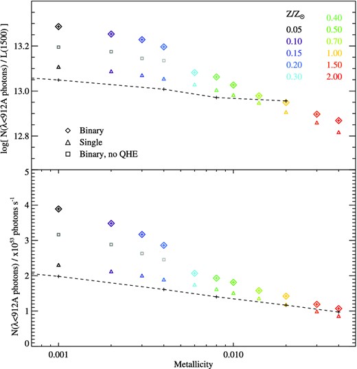
The steady-state ionizing flux from a continuously star-forming population, observed 100 Myr after the onset of star formation as a function of metallicity. Single-star models are shown in triangles, models incorporating binaries with diamonds. The upper panel shows the ratio of ionizing flux to continuum luminosity in units of photons s−1 per erg s−1 Å−1. The dashed line in the lower panel gives photon fluxes from the models of Schaerer (2003) and Raiter et al. (2010), given the correction factor necessary to match our assumed initial mass function (see Section 3.4). The dashed line in the upper panel shows the matching Raiter et al (2010) models for photon-to-continuum flux ratio.
3.4 Initial mass function
There is now observational evidence a small number of stars at M = 100–300 M⊙ in nearby star-forming regions (Crowther et al. 2010). While these are few in number, they are extremely luminous in the ultraviolet and thus provide a correction to the ionizing flux that is modestly metallicity dependent, resulting in a stellar population that is ‘top heavy’ relative to most previous work.
The range of stellar initial mass functions (IMFs) explored in Section 3.4. Our default IMF is number 3. The final two columns give the mean correction factor applied to the ionizing photon flux such that Nion(imfn) = bn Nion(imf3) for binary evolution models, while sn provides the same factor for single-star populations.
| α1 | α2 | |||
|---|---|---|---|---|
| Model | (0.1–0.5 M⊙) | (0.5 M⊙ to Mmax) | < bn > | < sn > |
| 1 | −1.30 | −2.00, Mmax=100 M⊙ | 2.55 | 2.68 |
| 2 | −1.30 | −2.00, Mmax=300 M⊙ | 4.05 | 4.37 |
| 3 | −1.30 | −2.35, Mmax=100 M⊙ | 1.00 | 1.00 |
| 4 | −1.30 | −2.35, Mmax=300 M⊙ | 1.45 | 1.54 |
| 5 | −2.35 | −2.35, Mmax=100 M⊙ | 0.77 | 0.74 |
| 6 | −1.30 | −2.70, Mmax=100 M⊙ | 0.32 | 0.30 |
| 7 | −1.30 | −2.70, Mmax=300 M⊙ | 0.41 | 0.41 |
To reproduce the Salpeter-like IMF (as used in e.g. Madau & Dickinson 2014), we select α1 = α2 = −2.35, Mmax = 100 M⊙ (model 5 in Table 1), while our standard assumed IMF has a break at M = 0.5 M⊙ with α1 = −1.30, α2 = −2.35 and an upper limit Mmax = 100 M⊙ (number 3). We also explore the effect of increasing the upper stellar initial mass limit, given our assumed power-law slopes (number 4). A steeper slope of α2 = −2.70 models the proposed IMF of Scalo (1986) (numbers 6 and 7), and we also consider the effect of a shallower ‘top-heavy’ IMF with α2 = −2.00 (numbers 1 and 2).
The impact of these variations in IMF on the ionizing flux output for a continuously star-forming population (after the initial stabilization phase), is shown in Fig. 7. As suggested in Section 3.3, our choice of IMF results in a ∼30 per cent excess in ionizing flux over that of model 5 for the same continuous star formation rate, while adopting a higher mass limit would give a flux ∼50 per cent higher than our standard model. As Fig. 6 showed, accounting for the broken power-law IMF, and for the stars with M = 0.1–1 M⊙ that were not included in the Schaerer (2003) models, we find good agreement with the predicted ionizing flux in that work for our single-star models, but a divergence in the binary models, particularly at low metallicities, where the effects of QHE are significant.
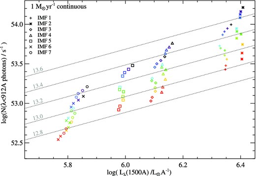
The ionizing photon flux from a continuous star formation episode, forming 1 M⊙ yr−1 and a binary stellar population, observed 108.5 yr after the onset of star formation, and its variation with metallicity and initial mass function. The key shows the initial mass function choice as given in Table 1. Dotted lines indicate lines of constant ionizing flux to continuum flux ratio in units of photons s−1/erg s−1 Å−1.
4 OBSERVABLES
4.1 UV spectral slope
At high redshifts, diagnostic features of stellar populations are redshifted out of observable wavebands and information may be limited to rest-frame ultraviolet emission. As Fig. 3 showed, the 1500 Å continuum flux is a reasonable, but not entirely unambiguous predictor of ionizing photon flux. The strong dependence of the latter on star formation history and of the former on stellar mass involved in the most recent starburst suggests that additional information may be required to make a reliable estimate of ionizing photon emission rate. One possible source of such information is the rest-frame ultraviolet spectral slope, β, defined though a power-law fit to the ultraviolet continuum of the form fλ ∝ λ−β.
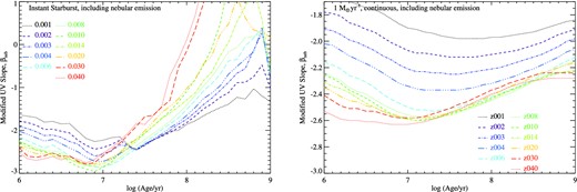
In Fig. 8, we examine the behaviour of the intrinsic stellar spectral slope as a function of age, metallicity and star formation history. In the continuous star formation case, the spectral slope (as measured by a linear fit to the 1250–1750 Å spectral region) shows little dependence on metallicity, and only modest dependence on stellar population age. At all metallicities, the ultraviolet spectral slope converges to β = −2.3 ± 0.10 at an age of ∼1 Gyr. In the context of distant galaxies, observed within the first billion years of star formation, it is interesting to note that below this age, the intrinsic spectral slope can reach values as steep as β = −2.9, with steeper slopes observed at younger ages and lower metallicities, although we note that the nebular continuum effects will modify the observed slope redwards of this value.
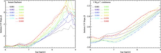
The intrinsic rest-frame ultraviolet spectral slope, arising from the stellar population and measured at 1500 Å, as a function of age for instantaneous and continuous star formation models (left and right, respectively). Note the two cases are plotted on different scales for clarity.
The general trend is similar, although more extreme, in the case of an ageing instantaneous starburst. These can reach slopes as steep as β = −3 in the case of a young, 10 Myr, stellar population at Z < 0.006, although such starburst only remains bluer than the continuous star formation case until 15–30 Myr after the starburst occurs, making this a relatively short-lived stage. It is notable that high-metallicity stellar populations redden much more rapidly than those at lower metallicities, which remain bluer than β = −2.0 more than 100 Myr after the starburst occurs.
So, if β is sensitive to star formation history, the question remains: can the rest-frame ultraviolet spectral slope clarify the predicted ionizing photon flux that should be inferred from a given 1500 Å luminosity? In Fig. 9, we explore this question, given two measurements of the intrinsic ultraviolet spectral slope – one, as above, based on fitting the 1250–1750 Å spectral region (as might be the case for very high redshift photometric or spectroscopic observations), and a second based on the 1500/2300 Å flux ratio (as measured, for example by the GALEXFUV − NUV colour at low redshift). The 912/1500 Å flux ratio is not strongly dependent on ultraviolet slope, but does vary with metallicity and star formation history. Interestingly, the slope between 1500 and 2300 Å may prove to be diagnostic of metallicity in a given star formation case; by contrast, the behaviour of the 1500 Å spectral slope is not strongly correlated with ionizing flux output, yielding a range of possible ionizing photon rates for a given β.
The continuum established by emission from hot, young stars as discussed above is modified both by an emission component from photoheated nebular gas, and scattering and absorption by interstellar dust before observation, both of which tend to redden the intrinsic stellar spectrum. This effect can lead to a significant difference between the intrinsic and apparent spectral slope, which is itself metallicity dependent. We caution that the results are somewhat sensitive to gas density and geometry but estimate the nebular emission component by processing our models through the publically available radiative transfer and photoionization code cloudy (Ferland et al. 2013), assuming a moderate gas density of 102 cm−2 and spherical geometry suitable for H ii regions (see Stanway et al. 2014, for discussion of the effect of gas density).
As shown in Fig. 10, for continuously star-forming systems, at near-solar metallicity and older than 10 Myr, the effect of nebular emission is relatively small, reddening the observed slopes by of order Δβ ± 0.05. The effect of the nebular component on low-metallicity spectra is stronger (up to Δβ ± 0.6 at 0.1 Z⊙) and persists to late times. As a result low-metallicity populations forming stars at a constant rate over time-scales of 100 Myr cannot reproduce the blue colours observed in the distant Universe, and either short lived or rising bursts are necessary to reproduce observations. The recent compilation of observational constraints by Duncan et al. (2014) suggests that the Lyman break galaxy population exhibits no clear evidence for a steepening of β with redshift, and a statistically significant but weak trend with ultraviolet luminosity, with more luminous (MUV ∼ −22) galaxies appearing Δβ ∼ 0.3 redder than faint galaxies (MUV ∼ −17) at z = 4. By contrast Bouwens et al. (2014) claim stronger evolution with both luminosity and age, with Δβ ∼ 0.7 over the same luminosity range at z = 4.
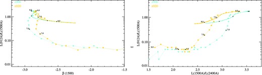
The 912/1500 Å flux ratios (in fλ), shown as a function of intrinsic rest-frame ultraviolet spectral slope measured at 1500 Å (left) and the 1500/2300 Å flux ratio (representative of continuum measurements, right). Starbursts are shown with dotted lines and continuous star formation models with solid lines. Two representative metallicities are shown for clarity.
The modified rest-frame ultraviolet spectral slope, arising from the stellar population, as in Fig. 8 and processed through a radiative transfer model to include the effects of nebular emission.
Observational data thus suggests that either the star-forming galaxies observed in the distant Universe are observed early in their starbursts, when the bluest slopes are expected, or that the evolution in observed rest-frame ultraviolet spectral slope is driven primarily by non-stellar factors - most likely variation in dust extinction (Wilkins et al. 2013; Duncan & Conselice 2015) - which would compromise inferences regarding ionizing photon flux based on 1500 Å continuum luminosity.
4.2 Helium ionization
Given that spectroscopic observations of high-redshifts systems are currently limited to the rest-frame ultraviolet, several ultraviolet emission lines with high ionization potentials have now been suggested as diagnostic. Prominent amongst these is the He ii 1640 Å feature, usually associated with the hard ionization spectra arising from AGN but also potentially indicative of a hard stellar spectrum such as might arise from metal-free, Population III stars. He ii 1640 Å has been observed in the stacked spectra of star-forming galaxies at z ∼ 3 (Shapley et al. 2003) and in individual cases at both higher and lower redshifts (e.g. Erb et al. 2010; Cassata et al. 2013), but remains undetected in a number of other cases (e.g. Dawson et al. 2004; Cai et al. 2011, 2015). If velocity broadened, it is usually interpreted as emission driven by Wolf–Rayet star winds, while narrow line emission may indicate photoionization of nebular gas by a hard, perhaps Population III, spectrum (although this interpretation is not unambiguous; Gräfener & Vink 2015).
Helium is energetically less favourable to excite into emission than atomic hydrogen, with a critical maximum wavelengths for ionizing photons of λc = 228 Å. Our calculated rates for production of photons with wavelengths shorter than this critical value is shown in Fig. 11 for both constant and instantaneous starbursts. Unsurprisingly, the time evolution of ionizing flux is broadly similar to that of hydrogen-ionizing photons. In the case of continuous, ongoing star formation, the ratio between flux of hydrogen and helium ionizing photons is fixed within 10 Myr of the onset of star formation. Interestingly, the flux ratio between hydrogen and He ii ionizing photons is strongly dependent on metallicity, varying by more than a magnitude over the range of metallicities considered here due to the harder spectrum of the ionizing flux at low metallicities in our models (particularly when the effects of QHE boost the population of luminous blue stars at relatively late times).
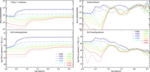
The rates of production of photons with energies exceeding the thresholds for He ii ionization for a range of ages and metallicities. The upper panels show the ratio of these photon production rates with those capable of ionizing hydrogen photons, i.e. Nion,HeII/Nion,H.
In the case of an ageing instantaneous starburst, the ionizing flux ratios are far less stable, and difficult to characterize as a function of metallicity and stellar population age. Particularly at young ages, the flux ratios are highly sensitive to metallicity, varying over more than 5 orders of magnitude in Nion,HeII/Nion,H, before converging to a slightly higher ratio at late ages than in the continuous star formation case. If the galaxies we observe at high redshift are indeed very young coeval starbursts, or are dominated by a single-age population, then the strength of He ii emission is unlikely to provide an unambiguous indication of the strength of the photon flux contributing to hydrogen reionization.
5 IMPLICATIONS FOR REIONIZATION
5.1 Critical star formation rate
The initial reionization of the Universe, occurring at the end of the cosmic dark ages and driven by the first ultraviolet-luminous sources, may well have been dominated by stellar populations with metallicities well below those considered here – perhaps metal-free, Population III stars (Schaerer 2003). Current indications from the cosmic microwave background radiation suggest that this may have occurred at zreion ∼ 9 (Planck Collaboration XIII 2015), beyond current spectroscopic limits for normal galaxies, and at an epoch where only photometric selection is currently possible. However, the Universe in the tail end of the reionization process, at z ∼ 5–6, is believed to be ionized to better than 99 per cent (Fan et al. 2006), and this state must be maintained against the rapid recombination of hydrogen atoms in the cold IGM (Madau et al. 1999; Madau & Dickinson 2014). The SEDs of spectroscopically confirmed ultraviolet-luminous galaxies in this redshift range are directly observable (e.g. Douglas et al. 2010; Stark et al. 2013; Dunlop et al. 2013), and the requirement that they maintain ionization of the IGM provides informative constraints on their Lyman-continuum flux.
As discussed in Section 3, the production of hydrogen-ionizing photons is a sensitive function of stellar population age, metallicity and star formation history. However, given reasonable assumptions for these parameters, it is possible to constrain the volume-averaged star formation rate (and 1500 Å flux density) required to maintain the ionization of the IGM as a function of redshift. To do so, we define three models to provide estimates for the photon production rate:
Case A: Constant star formation, seen at an age of 100 Myr with a total stellar mass of 108 M⊙ formed at a rate of 1 M⊙ yr−1, and photon production rates of Nion,H =(1.0–3.9) × 1053 s−1 using our binary star formation models, dependent on metallicity.
Case B: An equal age starburst, with a total stellar mass of 108 M⊙, seen 10 Myr after the onset of star formation, with photon production rates Nion,H = (0.8–8.9) × 1053 s−1, corresponding to a time averaged star formation rate of 10 M⊙ yr−1.
Case C: An equal age starburst, with a total stellar mass of 108 M⊙, seen 30 Myr after the onset of star formation, with photon production rates Nion,H =(0.10–0.16) × 1053 s−1, corresponding to a time averaged star formation rate of 3.3 M⊙ yr−1.
While these are, of course, selected snapshots in star formation history, they are indicative of the differences in behaviour between different models. The output properties arising from each scenario is illustrated in Fig. 12. In each case, the same total stellar mass would be measured using an SED fitting technique, and the star formation rate would likely be inferred from a combination of that, template-dependent, procedure and a fixed conversion factor applied to the rest-frame ultraviolet luminosity. As the figure demonstrates, the inferred star formation rates and ionizing photon fluxes are far from easy to interpret. Case B (the 10 Myr starburst) shows a rest ultraviolet luminosity only two times higher than that of case A (continuous star formation), despite having a time averaged star formation rate ten times higher over its stellar lifetime. The ionizing photon fluxes in these two scenarios are also similar, differing only by a factor of ∼2, but with the higher luminosity case yielding the lower photon flux. By contrast, while cases B and C (the two ageing starbursts) differ by a factor of ∼3 in ultraviolet luminosity, similar to the difference in their volume-averaged star formation rate, they differ by a factor of ∼12 in ionizing photon flux. Remembering that these represent only three scenarios, and that true star formation histories are likely a more complex combination of continuous, declining or instantaneous star formation, it is clear that a great deal of caution must be exercised in interpreting the ionizing flux based on ultraviolet continuum.
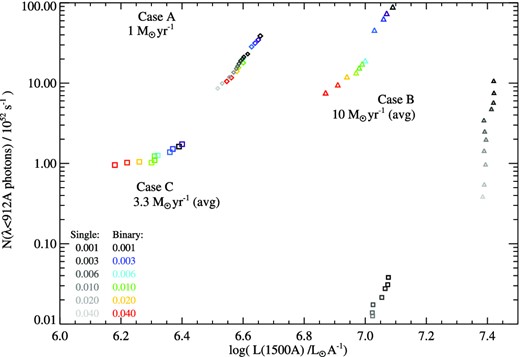
The rates of production of hydrogen-ionizing photons and rest-frame ultraviolet luminosity for three scenarios generating the same stellar mass, 108 M⊙. The three star formation history cases described in Section 5.1 are shown with different symbols, with binary models coloured by metallicity. The results of our single-star models are shown in grey-scale for comparison.
In Fig. 13, we use our three fiducial star formation history cases to calculate the required, volume-averaged 1500 Å continuum luminosity density to maintain the ionization of the Universe, as a function of redshift, given our predictions for Nion,H, and assuming CH = 3, fesc = 0.2 and T = 104 K at z = 7. In all but case A, we require a higher star formation rate density and luminosity density to maintain the ionization state than those estimated by Madau et al. (1999) or Topping & Schull (2015), due to the short ionizing lifetimes of ageing starbursts. However, the critical 1500 Å luminosity density is broadly consistent with that of Madau et al. (1999) for the continuous star formation case at near-solar metallicity, and we actually require a lower 1500 Å luminosity density for continuous star formation at the lowest metallicities.
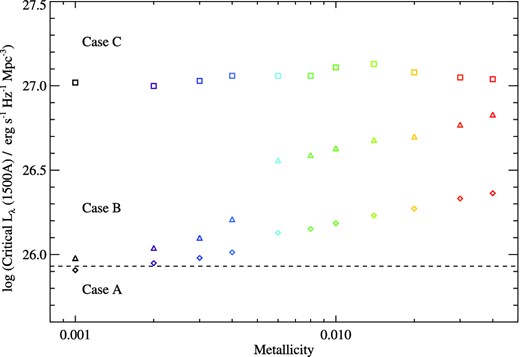
The critical average ultraviolet flux density per unit volume required to maintain the ionization balance of the Universe at z = 7, assuming CH = 3, fesc = 0.2 and T = 104 K (see Section 5.1) and the three fiducial star formation histories assumed in Fig. 12 and Section 5.1. The dashed line indicates the critical luminosity density of Madau et al. (1999), assuming LUV = 8 × 1027 (SFR/M⊙ yr−1) erg s−1 Hz−1 and a Salpeter IMF (Madau et al 1998).
5.2 Lower mass limits
The number density and luminosity distribution of the rest-frame ultraviolet-luminous, star-forming galaxy population is now well established at z ∼ 3–6, and their characteristics constrained (subject to small number statistics and possible contamination and completeness concerns, see Stanway, Bremer & Lehnert 2008) based on colour-selected candidates at z ∼ 7–10 (Bouwens et al. 2015). While these luminosity functions likely underestimate the number of star-forming galaxies at a given mass, and the intrinsic emission of each, due to the effects of dust extinction, they provide a good measure of the number of galaxies with sufficiently low dust obscuration to irradiate their surroundings with ionizing photons. By summing the volume-averaged flux density emitted by galaxies at each luminosity, down to some minimum luminosity, and considering the relations demonstrated in Section 4, the ionizing photon flux arising from the galaxy's stellar population can be calculated. The minimum luminosity (or equivalently mass) limit appropriate for this procedure is a matter of some uncertainty, and may well vary with redshift, as galaxies grow sufficiently massive to collapse under their own gravitation and begin star formation, or massive enough to retain their gas supply against the stellar winds driven by intense starbursts. While some authors have chosen only to consider galaxies which exceed an absolute magnitude MUV = −15 (e.g. Madau & Dickinson 2014), others integrate down to MUV = −10 (e.g. Robertson et al. 2015) or into the regime at which dwarf galaxies and globular clusters meet (see Muñoz & Loeb 2011, and discussion therein). Given the steepness of the low-luminosity end of the luminosity functions measured at z > 3 (Reddy & Steidel 2009; Bouwens et al. 2015), a relatively small difference in minimum mass can give rise to a strong difference in ionizing flux.
In Figs 14 and 15, we consider the three star formation scenarios introduced in Section 5.1, and in each case determine the minimum galaxy mass required to produce the critical 1500 Å luminosity densities shown in Fig. 13 and thus maintain the ionization state of the IGM. We continue to assume CH = 3, fesc = 0.2 and T = 104 K, and scale the required flux to each observed redshift as specified in the prescription of Topping & Schull (2015). We use the Lyman break galaxy luminosity functions derived by Bouwens et al. (2015) as a function of redshift, based on the largest currently available set of deep field observational data, and assume these Schechter (1976) function parametrizations extend to lower luminosities, beyond current observable limits (although note that z > 6 Lyman α emitting galaxies may deviate from such a Schecter function; Matthee et al. 2015).
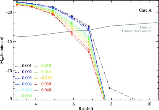
The lowest luminosity galaxies required to maintain the ionization of the intergalactic medium as a function of redshift and metallicity, assuming the integrated 1500 Å ultraviolet luminosity density given by the Lyman break galaxy luminosity functions of Bouwens et al. (2015). The limit of the deepest observations used by Bouwens et al is shown with a solid line. Models are shown for continuous star formation (case A, see Section 5.1 for details).
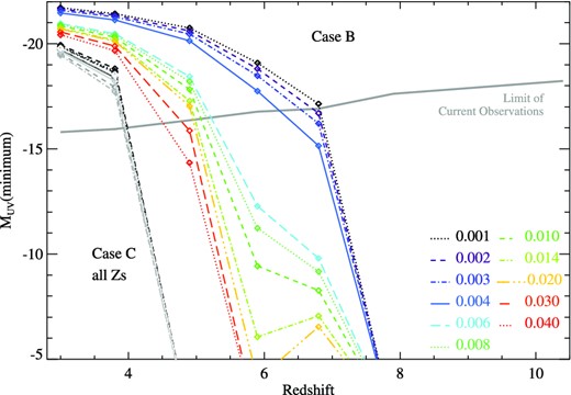
As in Fig. 14 but assuming Lyman break galaxies can typically be described by 10 Myr or 30 Myr old starburst models (i.e. case B or C). Case C is shown in grey-scale and exhibits very little metallicity dependence.
If the Lyman break galaxy population is dominated by regions with ongoing, continuous star formation exceeding ∼10 Myr in age (case A), our models suggest that the galaxy population already observed in existing deep field observations is sufficient to maintain the ionization state of the Universe at z < 7, but that doing so at z ∼ 8 would require both a low-metallicity stellar population (Z < 0.2 Z⊙) and a galaxy luminosity distribution that extends down as far as MUV = −10 to 12. At redshifts higher than this, our models cannot produce the critical ionizing flux, given current galaxy population observations, suggesting either that the luminosity function steepens still further, that the conditions in the IGM are evolving with redshift, or that exceptionally low metallicity, Population III stellar populations may become important.
In the case of instantaneous starbursts, ageing passively and typically observed at 10 or 30 Myr after the burst (cases B and C), the maintenance of ionization balance with current galaxy luminosity distributions becomes challenging at redshifts above z = 4.5 and z = 6, respectively, except at the lowest metallicities considered here. While the possibility that young starbursts may dominate at z ∼ 5–7 remains present (particularly given the blue observed ultraviolet slopes, Section 4.1), this would suggest substantial evolution in the IGM properties (perhaps most likely the escape fraction, fesc, see Section 5.3) or in the metallicity of the stellar population. We note that the critical ionizing flux is usually calculated as a lifetime average for the stars formed, whereas we are taking a somewhat different approach here, directly converting the rest-frame ultraviolet continuum in observed galaxies to a photon flux assuming different conversion factors. Given the vast uncertainty in actual star formation history the detailed conversion factors may well differ, but these calculations give some indication of possible constraints given assumptions about the dominant, observed stellar population.
5.3 Lyman-continuum escape fraction
We have already considered the L912/L1500 ratio as a function of ultraviolet spectral slope, determining in Section 4.1 that it is difficult to predict or extrapolate ionizing flux levels from observations longwards of the Lyman limit. However measurements of this quantity now exist, both directly through observations of Lyman-continuum photons from distant galaxies and indirectly from the ionization state of the IGM as traced by the Lyman α forest. The interpretation of these measurements in the context of stellar population models is complicated by our lack of knowledge of fesc, the fraction of Lyman-continuum photons that escape local absorption and reach the IGM. Most of the ionizing flux emitted by stars will be absorbed by nearby gas and dust and re-emitted at other wavelengths, predominantly in a continuum component and strong emission lines such as H α. Only a fraction of the intrinsic ionizing radiation arising from the stellar population will escape and this factor is uncertain as we cannot measure the ionizing flux directly. However if a stellar population, or range of stellar populations, is assumed, then constraints can be placed on fesc.
Models of reionization have led to suggestions that the fraction of photons escaping from high-redshift galaxies must be very high. Fontanot et al. (2014) suggest fesc = 0.1–0.3 is required for stars in galaxies to reionize the Universe, while Haardt & Madau (2012) use a redshift-dependent fesc for their work which is even greater. Such high escape fractions are contentious. High-resolution simulations of galaxy properties, rather than reionization itself, struggle to produce high values, finding a typical fesc ∼ 5 per cent (Ma et al. 2015).
Observations in the local Universe also favour a low value, suggesting that only very massive star-forming regions in galaxies leak a significant fraction of photons into the diffuse interstellar medium (Oey & Kennicutt 1997; Eldridge & Relaño 2011). It is unknown what fraction of these can then escape into the IGM. Observations of so-called ‘Lyman break analogues’ – local, ultraviolet-luminous galaxies which mirror the physical conditions of more distant sources (Stanway & Davies 2014)– have suggested that the ‘leakiness’ of galaxies to Lyman-continuum photons is strongly correlated to their compactness and the speed of galaxy-scale outflows driven by the galaxy-wide starburst (Alexandroff et al. 2015). Given that both compactness and occurrence of outflows appear to be common in the distant Universe (e.g. Oesch et al. 2010; Steidel et al. 2010), it might be expected that high escape fractions are possible. However, simulations by Cen & Kimm (2015) suggest that the picture is more complex still, with a broad range of escape fractions present within a given galaxy population, and large samples required to accurately recover them.
At higher redshift (z > 2), where the ionizing continuum has redshifted into the optical, it becomes possible to measure the amount of leaking continuum directly, but, given the difficulty of doing so, only for small samples of galaxies. Unfortunately, by z ∼ 4 the mean opacity of the IGM becomes very high, leaving a narrow redshift window in which measurements can be made. Only rare z = 3–4 LBGs have an estimated fesc of 0.25–1, with the majority undetected in deep Lyman-continuum imaging (Vanzella et al. 2012; Vanzella et al. 2015). Shapley et al. (2006) detected two sources, with a sample-averaged fesc ∼ 14 per cent, while most studies (e.g. Mostardi et al. 2013; Nestor et al. 2013) suggest that LBGs at z ∼ 2–4 have a relatively modest fesc of 0.05–0.07. However such conclusions are inevitably based on assumptions regarding the emitted spectrum and its comparison with observations.
In Fig. 16, we compare the ionizing photon flux predicted by our models, given the integrated flux arising from the observed 1500 Å luminosity functions of Lyman break galaxies as a function of redshift (Reddy & Steidel 2009; Bouwens et al. 2015), to the ionizing photon flux inferred by Becker & Bolton (2013) based on measurements of the Lyman α forest at z ∼ 2–5. We integrate the galaxy population to an absolute magnitude limit MUV = −10, and again consider the three star formation histories introduced in Section 5.1. While it is possible that older stellar populations exist at z < 5 than was possible at earlier times, if these are experiencing ongoing star formation then case A will remain a good description even at ages >1 Gyr (see Fig. 4). As the figure demonstrates, a population of sudden, coeval starbursts observed at ∼30 Myr post-burst (case C) would require an escape fraction fesc ∼ 1 to reproduce the observed ionizing flux density at z ∼ 2–5, suggesting that this is an unlikely model at these late times. By contrast, very young starbursts (case B), bursts with rising star formation histories that would imitate such a scenario, and the continuous star formation case (case A) require only a relatively small escape fraction.
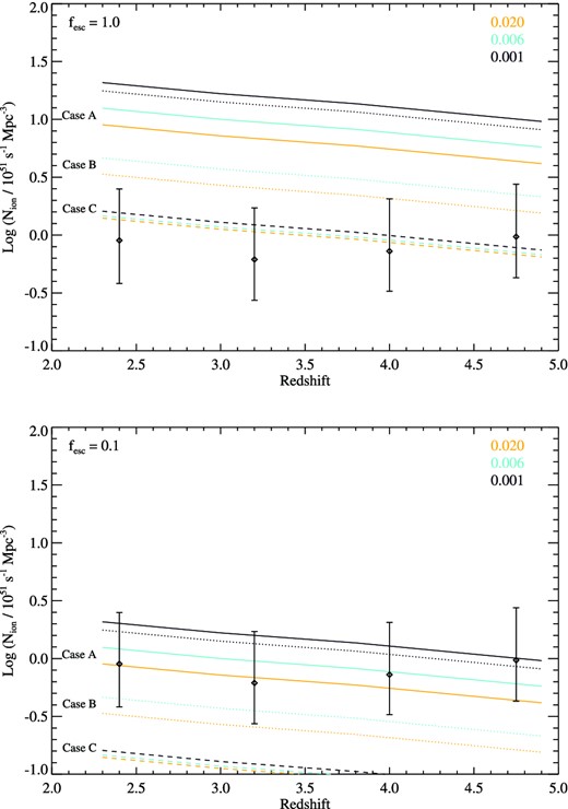
The ionizing photon flux generated by the Lyman break galaxy population, assuming the 1500 Å ultraviolet luminosity density given by the Lyman break galaxy luminosity functions of Bouwens et al. (2015) and Reddy & Steidel (2009) and integrated down to MUV = −10, compared to that required to reproduce the observed ionization of the IGM at intermediate redshift as measured by Becker & Bolton (2013, diamonds). Models are shown for three representative metallicities, two values of the Lyman-continuum escape fraction and the star formation cases defined in Section 5.1.
The best-fitting escape fractions, assuming a constant star formation rate, are shown in Fig. 17 as a function of redshift, and given at three different metallicities. While uncertainties on the observational data remain large, there is slight evidence for a trend to higher escape fractions at z > 4.5, although this may be evidence instead of an evolution towards lower metallicities. Stellar models at Z = 0.006 and Z = 0.001 (0.3 and 0.1 solar) require an escape fraction ∼65 and 40 per cent of that required at Z = 0.020 (solar), respectively, where the best-fitting escape fractions (from the stellar emission to the IGM) at Z = 0.020 are fesc ∼ 0.08–0.24, rising with redshift. Thus, models a few tenths of solar metallicity provide self-consistent agreement between observed galaxy luminosity functions, ionization of the IGM and estimated escape fractions at z ∼ 3.
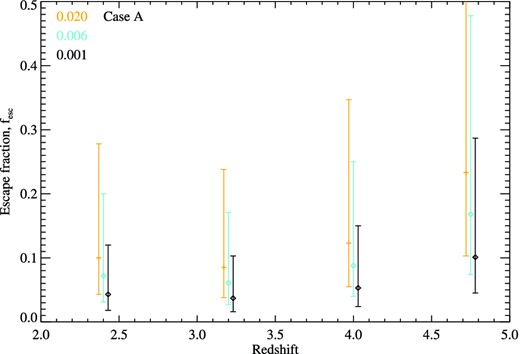
The best-fitting escape fraction required to reproduce the Lyman α forest measurements of Becker & Bolton (2013), given the observed Lyman break galaxy luminosity functions, and assuming a constant star formation rate (case A). Escape fractions are shown at three metallicities, slightly offset for clarity.
6 CONCLUSIONS
We have calculated the ionizing photon flux from young stellar populations, as given by stellar population synthesis models incorporating detailed binary evolution pathways. We have explored how this flux depends on the history and properties of star formation in a galaxy, and considered the implications of the resultant uncertainty for the reionization of the Universe at the end of the cosmic dark ages.
Our main numerical results are presented in Table 2 and can be summarized as follows:
A stellar population undergoing constant star formation and incorporating binaries produces a higher hydrogen-ionizing flux than that of a population assumed to evolve purely through single-star evolution pathways. The excess in the binary case is ∼60 per cent of the single-star flux at modestly sub-solar (0.1–0.2 Z⊙) metallicities.
Table 2.Observable and inferred parameters from our model stellar populations for a system undergoing star formation at a constant rate observed at an age of 100 Myr after the onset of star formation at which point the fluxes have stabilized (case A), and for instantaneous starburst models of initial stellar mass 106 M⊙ observed at 10 Myr (case B) and 30 Myr (case C) after the burst. Star formation rates are given in M⊙ yr−1, luminosities in erg s−1 Hz−1 and photon rates in s−1. βint is the intrinsic 1500 Å spectral slope arising from the stellar continuum. All results are quoted for binary stellar populations and for our standard initial mass function.
Z |$\log N_\mathrm{ion}$| |$\log {L_\mathrm{1500}}$| |$\log [\frac{N_\mathrm{ion}}{L_{1500}}]$| |$\log [\frac{N_\mathrm{ion,He\,II}}{L_{1500}}]$| |$\log [\frac{N_\mathrm{ion,C\,III}}{L_{1500}}]$| |$\frac{L_{912}}{L_{1500}}$| βint Case A 0.001 53.59 28.12 25.47 22.29 23.73 2.35 −2.55 0.002 53.54 28.11 25.43 22.18 23.62 2.27 −2.60 0.003 53.50 28.10 25.40 22.16 23.55 2.22 −2.64 0.004 53.45 28.09 25.37 21.51 23.36 2.16 −2.68 0.006 53.31 28.06 25.25 21.17 23.15 1.87 −2.66 0.008 53.28 28.05 25.23 20.97 23.06 1.84 −2.64 0.010 53.25 28.06 25.19 20.82 22.86 1.76 −2.61 0.014 53.19 28.04 25.15 20.88 22.75 1.70 −2.58 0.020 53.15 28.04 25.11 20.75 22.58 1.70 −2.52 0.030 53.07 28.02 25.05 20.53 22.46 1.70 −2.47 0.040 53.02 28.01 25.02 20.41 22.37 1.79 −2.47 Case B 0.001 51.95 28.55 23.40 20.43 21.77 3.73 −2.64 0.002 51.87 28.53 23.34 20.09 21.63 3.54 −2.74 0.003 51.80 28.52 23.28 19.93 21.51 3.41 −2.82 0.004 51.66 28.49 23.17 19.21 21.25 3.33 −2.90 0.006 51.28 28.46 22.82 19.07 21.02 2.95 −2.93 0.008 51.24 28.45 22.79 18.98 21.02 2.87 −2.90 0.010 51.19 28.44 22.75 19.12 20.93 2.76 −2.87 0.014 51.13 28.43 22.70 19.21 20.98 2.65 −2.82 0.020 51.08 28.40 22.68 19.03 20.97 2.60 −2.77 0.030 50.98 28.37 22.61 18.86 20.98 2.54 −2.65 0.040 50.88 28.33 22.55 18.67 20.96 2.62 −2.61 Case C 0.001 50.21 27.85 22.36 19.56 20.86 2.84 −2.39 0.002 50.24 27.86 22.38 19.53 20.86 2.71 −2.38 0.003 50.18 27.83 22.35 19.48 20.80 2.65 −2.37 0.004 50.14 27.82 22.32 18.65 20.39 2.57 −2.37 0.006 50.10 27.78 22.32 18.70 20.41 2.22 −2.27 0.008 50.09 27.77 22.32 18.71 20.44 2.16 −2.19 0.010 50.04 27.77 22.27 17.90 20.05 2.11 −2.15 0.014 50.01 27.76 22.25 17.88 20.07 2.03 −2.16 0.020 50.02 27.72 22.30 17.93 20.10 2.00 −2.03 0.030 50.01 27.68 22.33 17.89 20.16 1.97 −1.82 0.040 49.98 27.64 22.34 17.84 20.12 2.06 −1.75 Z |$\log N_\mathrm{ion}$| |$\log {L_\mathrm{1500}}$| |$\log [\frac{N_\mathrm{ion}}{L_{1500}}]$| |$\log [\frac{N_\mathrm{ion,He\,II}}{L_{1500}}]$| |$\log [\frac{N_\mathrm{ion,C\,III}}{L_{1500}}]$| |$\frac{L_{912}}{L_{1500}}$| βint Case A 0.001 53.59 28.12 25.47 22.29 23.73 2.35 −2.55 0.002 53.54 28.11 25.43 22.18 23.62 2.27 −2.60 0.003 53.50 28.10 25.40 22.16 23.55 2.22 −2.64 0.004 53.45 28.09 25.37 21.51 23.36 2.16 −2.68 0.006 53.31 28.06 25.25 21.17 23.15 1.87 −2.66 0.008 53.28 28.05 25.23 20.97 23.06 1.84 −2.64 0.010 53.25 28.06 25.19 20.82 22.86 1.76 −2.61 0.014 53.19 28.04 25.15 20.88 22.75 1.70 −2.58 0.020 53.15 28.04 25.11 20.75 22.58 1.70 −2.52 0.030 53.07 28.02 25.05 20.53 22.46 1.70 −2.47 0.040 53.02 28.01 25.02 20.41 22.37 1.79 −2.47 Case B 0.001 51.95 28.55 23.40 20.43 21.77 3.73 −2.64 0.002 51.87 28.53 23.34 20.09 21.63 3.54 −2.74 0.003 51.80 28.52 23.28 19.93 21.51 3.41 −2.82 0.004 51.66 28.49 23.17 19.21 21.25 3.33 −2.90 0.006 51.28 28.46 22.82 19.07 21.02 2.95 −2.93 0.008 51.24 28.45 22.79 18.98 21.02 2.87 −2.90 0.010 51.19 28.44 22.75 19.12 20.93 2.76 −2.87 0.014 51.13 28.43 22.70 19.21 20.98 2.65 −2.82 0.020 51.08 28.40 22.68 19.03 20.97 2.60 −2.77 0.030 50.98 28.37 22.61 18.86 20.98 2.54 −2.65 0.040 50.88 28.33 22.55 18.67 20.96 2.62 −2.61 Case C 0.001 50.21 27.85 22.36 19.56 20.86 2.84 −2.39 0.002 50.24 27.86 22.38 19.53 20.86 2.71 −2.38 0.003 50.18 27.83 22.35 19.48 20.80 2.65 −2.37 0.004 50.14 27.82 22.32 18.65 20.39 2.57 −2.37 0.006 50.10 27.78 22.32 18.70 20.41 2.22 −2.27 0.008 50.09 27.77 22.32 18.71 20.44 2.16 −2.19 0.010 50.04 27.77 22.27 17.90 20.05 2.11 −2.15 0.014 50.01 27.76 22.25 17.88 20.07 2.03 −2.16 0.020 50.02 27.72 22.30 17.93 20.10 2.00 −2.03 0.030 50.01 27.68 22.33 17.89 20.16 1.97 −1.82 0.040 49.98 27.64 22.34 17.84 20.12 2.06 −1.75 Table 2.Observable and inferred parameters from our model stellar populations for a system undergoing star formation at a constant rate observed at an age of 100 Myr after the onset of star formation at which point the fluxes have stabilized (case A), and for instantaneous starburst models of initial stellar mass 106 M⊙ observed at 10 Myr (case B) and 30 Myr (case C) after the burst. Star formation rates are given in M⊙ yr−1, luminosities in erg s−1 Hz−1 and photon rates in s−1. βint is the intrinsic 1500 Å spectral slope arising from the stellar continuum. All results are quoted for binary stellar populations and for our standard initial mass function.
Z |$\log N_\mathrm{ion}$| |$\log {L_\mathrm{1500}}$| |$\log [\frac{N_\mathrm{ion}}{L_{1500}}]$| |$\log [\frac{N_\mathrm{ion,He\,II}}{L_{1500}}]$| |$\log [\frac{N_\mathrm{ion,C\,III}}{L_{1500}}]$| |$\frac{L_{912}}{L_{1500}}$| βint Case A 0.001 53.59 28.12 25.47 22.29 23.73 2.35 −2.55 0.002 53.54 28.11 25.43 22.18 23.62 2.27 −2.60 0.003 53.50 28.10 25.40 22.16 23.55 2.22 −2.64 0.004 53.45 28.09 25.37 21.51 23.36 2.16 −2.68 0.006 53.31 28.06 25.25 21.17 23.15 1.87 −2.66 0.008 53.28 28.05 25.23 20.97 23.06 1.84 −2.64 0.010 53.25 28.06 25.19 20.82 22.86 1.76 −2.61 0.014 53.19 28.04 25.15 20.88 22.75 1.70 −2.58 0.020 53.15 28.04 25.11 20.75 22.58 1.70 −2.52 0.030 53.07 28.02 25.05 20.53 22.46 1.70 −2.47 0.040 53.02 28.01 25.02 20.41 22.37 1.79 −2.47 Case B 0.001 51.95 28.55 23.40 20.43 21.77 3.73 −2.64 0.002 51.87 28.53 23.34 20.09 21.63 3.54 −2.74 0.003 51.80 28.52 23.28 19.93 21.51 3.41 −2.82 0.004 51.66 28.49 23.17 19.21 21.25 3.33 −2.90 0.006 51.28 28.46 22.82 19.07 21.02 2.95 −2.93 0.008 51.24 28.45 22.79 18.98 21.02 2.87 −2.90 0.010 51.19 28.44 22.75 19.12 20.93 2.76 −2.87 0.014 51.13 28.43 22.70 19.21 20.98 2.65 −2.82 0.020 51.08 28.40 22.68 19.03 20.97 2.60 −2.77 0.030 50.98 28.37 22.61 18.86 20.98 2.54 −2.65 0.040 50.88 28.33 22.55 18.67 20.96 2.62 −2.61 Case C 0.001 50.21 27.85 22.36 19.56 20.86 2.84 −2.39 0.002 50.24 27.86 22.38 19.53 20.86 2.71 −2.38 0.003 50.18 27.83 22.35 19.48 20.80 2.65 −2.37 0.004 50.14 27.82 22.32 18.65 20.39 2.57 −2.37 0.006 50.10 27.78 22.32 18.70 20.41 2.22 −2.27 0.008 50.09 27.77 22.32 18.71 20.44 2.16 −2.19 0.010 50.04 27.77 22.27 17.90 20.05 2.11 −2.15 0.014 50.01 27.76 22.25 17.88 20.07 2.03 −2.16 0.020 50.02 27.72 22.30 17.93 20.10 2.00 −2.03 0.030 50.01 27.68 22.33 17.89 20.16 1.97 −1.82 0.040 49.98 27.64 22.34 17.84 20.12 2.06 −1.75 Z |$\log N_\mathrm{ion}$| |$\log {L_\mathrm{1500}}$| |$\log [\frac{N_\mathrm{ion}}{L_{1500}}]$| |$\log [\frac{N_\mathrm{ion,He\,II}}{L_{1500}}]$| |$\log [\frac{N_\mathrm{ion,C\,III}}{L_{1500}}]$| |$\frac{L_{912}}{L_{1500}}$| βint Case A 0.001 53.59 28.12 25.47 22.29 23.73 2.35 −2.55 0.002 53.54 28.11 25.43 22.18 23.62 2.27 −2.60 0.003 53.50 28.10 25.40 22.16 23.55 2.22 −2.64 0.004 53.45 28.09 25.37 21.51 23.36 2.16 −2.68 0.006 53.31 28.06 25.25 21.17 23.15 1.87 −2.66 0.008 53.28 28.05 25.23 20.97 23.06 1.84 −2.64 0.010 53.25 28.06 25.19 20.82 22.86 1.76 −2.61 0.014 53.19 28.04 25.15 20.88 22.75 1.70 −2.58 0.020 53.15 28.04 25.11 20.75 22.58 1.70 −2.52 0.030 53.07 28.02 25.05 20.53 22.46 1.70 −2.47 0.040 53.02 28.01 25.02 20.41 22.37 1.79 −2.47 Case B 0.001 51.95 28.55 23.40 20.43 21.77 3.73 −2.64 0.002 51.87 28.53 23.34 20.09 21.63 3.54 −2.74 0.003 51.80 28.52 23.28 19.93 21.51 3.41 −2.82 0.004 51.66 28.49 23.17 19.21 21.25 3.33 −2.90 0.006 51.28 28.46 22.82 19.07 21.02 2.95 −2.93 0.008 51.24 28.45 22.79 18.98 21.02 2.87 −2.90 0.010 51.19 28.44 22.75 19.12 20.93 2.76 −2.87 0.014 51.13 28.43 22.70 19.21 20.98 2.65 −2.82 0.020 51.08 28.40 22.68 19.03 20.97 2.60 −2.77 0.030 50.98 28.37 22.61 18.86 20.98 2.54 −2.65 0.040 50.88 28.33 22.55 18.67 20.96 2.62 −2.61 Case C 0.001 50.21 27.85 22.36 19.56 20.86 2.84 −2.39 0.002 50.24 27.86 22.38 19.53 20.86 2.71 −2.38 0.003 50.18 27.83 22.35 19.48 20.80 2.65 −2.37 0.004 50.14 27.82 22.32 18.65 20.39 2.57 −2.37 0.006 50.10 27.78 22.32 18.70 20.41 2.22 −2.27 0.008 50.09 27.77 22.32 18.71 20.44 2.16 −2.19 0.010 50.04 27.77 22.27 17.90 20.05 2.11 −2.15 0.014 50.01 27.76 22.25 17.88 20.07 2.03 −2.16 0.020 50.02 27.72 22.30 17.93 20.10 2.00 −2.03 0.030 50.01 27.68 22.33 17.89 20.16 1.97 −1.82 0.040 49.98 27.64 22.34 17.84 20.12 2.06 −1.75 Single age stellar populations observed post-starburst show rapid evolution in their ionizing photon flux, which is generally lower than in the constant star formation case. However, binary pathways prolong the period over which a starburst generates an ionizing photon flux, with photon production rates ∼100 times higher at ages of 10-30 Myr than in the single-star case.
Stellar populations show a strong trend in ionizing flux production with metallicity (in the range 0.05–2 Z⊙), with low-metallicity populations producing a higher ionizing flux at a given star formation rate. For a galaxy forming 1 M⊙ yr−1, observed at >100 Myr after the onset of star formation, we predict a production rate of photons capable of ionizing hydrogen, Nion = 1.4 × 1053 s−1 at Z = Z⊙ and 3.5 × 1053 s−1 at 0.1 Z⊙ assuming our standard IMF, as shown in Table 2. At solar and super-solar metallicities, binary pathways have very little effect on the photon production rate.
The ultraviolet spectral slope, β is an unreliable indicator of ionizing photon flux, showing strong dependence on recent star formation history and metallicity, as well as being subject to uncertainties in the dust extinction law. Young starbursts with relatively little gas and dust would straightforwardly match the steep spectral slopes (β < −2.5) seen in high-redshift galaxy samples.
The production of photons capable of ionizing He ii maintains a constant ratio to the hydrogen-ionizing flux for ongoing star formation, although this takes longer to become established at solar and super-solar metallicities than at low metallicity (∼30 Myr compared to a few Myr). For ageing single-burst stellar populations, the ratios of these photons show strong variation with stellar population age.
The ionizing flux required to maintain the ionization state of the IGM yields a critical star formation rate dependent on star formation history and metallicity. In the case of continuous star formation, binary models produce similar estimates for the critical star formation rate for reionization to older models including single stars. However, we note that the star formation history can change the required time- and volume-averaged star formation rate to reach the ionizing photon threshold by more than an order of magnitude.
We find that, assuming constant star formation, currently observed galaxy luminosity functions must be integrated down to a lower absolute magnitude limit of MUV ∼ −10 to maintain the ionization limit of the Universe at z > 7 (depending on stellar metallicity, assuming fesc = 0.2). Beyond this redshift, or at lower escape fractions, maintaining the ionization balance of the Universe, let alone the reionization process, becomes challenging. In the case of young starbursts, doing so becomes challenging at redshifts as low as z ∼ 4.5.
Assuming the constant star formation case, we find that escape fractions fesc ranging from a few per cent (at sub-solar metallicities) up to 24 per cent (at solar metallicity) are required to recover the ionizing flux observed in the IGM at z ∼ 2–5, based on observed Lyman break galaxy luminosity functions. Lower escape fractions by a factor of 2–3 required at metallicities of a tenth solar, relative to solar.
While the models discussed here necessarily explore only a subset of possible characteristics of star formation in the distant Universe, it is clear that the interpretation of 1500 Å continuum luminosities as indicative of ionizing flux, or indeed of other spectral features such as He ii or C iv emission, should be approached with caution. The very limited observational constraints on these underlying characteristics of the stellar population can give rise to almost an order of magnitude uncertainty in the ionizing flux, and this is most strongly affected by the star formation history. If a rising fraction of the Lyman break galaxy population is powered by very young starbursts with increasing redshifts, then currently observed galaxy populations may struggle to reproduce the ionizing flux necessary to maintain ionization balance at z > 5. None the less, it is both interesting and encouraging that, given constant star formation, extrapolation of the existing galaxy population to a reasonable lower mass limit confirms that Lyman break galaxies are capable of sustaining the ionization balance of the IGM at z < 7, and perhaps as high as z ∼ 8, without invoking exceptionally high escape fractions, steep luminosity functions or low, Population III metallicities.
ERS acknowledges support for this work from the University of Warwick Research Development Fund. ERS also acknowledges support from Science and Technology Facilities Council (STFC) consolidated grant ST/L000733/1. JJE acknowledges support from the University of Auckland. We thank Martin Haehnelt for useful and interesting discussions. We make use of version 13.03 of Cloudy, last described by Ferland et al. (2013). The authors wish to acknowledge the contribution of the NeSI high-performance computing facilities and the staff at the Centre for eResearch at the University of Auckland. New Zealands national facilities are provided by the New Zealand eScience Infrastructure (NeSI) and funded jointly by NeSIs collaborator institutions and through the Ministry of Business, Innovation and Employments Infrastructure programme. URL: http://www.nesi.org.nz.nz.
REFERENCES
