


Abstract
We investigate the formation of hydrogen cyanide (HCN) in the inner circumstellar envelopes of thermally pulsing asymptotic giant branch (TP-AGB) stars. A dynamic model for periodically shocked atmospheres, which includes an extended chemo-kinetic network, is for the first time coupled to detailed evolutionary tracks for the TP-AGB phase computed with the colibri code. We carried out a calibration of the main shock parameters (the shock formation radius rs,0 and the effective adiabatic index |$\gamma _{\rm ad}^{\rm eff}$|) using the circumstellar HCN abundances recently measured for a populous sample of pulsating TP-AGB stars. Our models recover the range of the observed HCN concentrations as a function of the mass-loss rates, and successfully reproduce the systematic increase of HCN moving along the M-S-C chemical sequence of TP-AGB stars, which traces the increase of the surface C/O ratio. The chemical calibration brings along two important implications for the physical properties of the pulsation-induced shocks: (i) the first shock should emerge very close to the photosphere (rs,0 ≃ 1R), and (ii) shocks are expected to have a dominant isothermal character |$(\gamma _{\rm ad}^{\rm eff}\simeq 1)$| in the denser region close to the star (within ∼3–4R), implying that radiative processes should be quite efficient. Our analysis also suggests that the HCN concentrations in the inner circumstellar envelopes are critically affected by the H–H2 chemistry during the post-shock relaxation stages. Given the notable sensitiveness of the results to stellar parameters, this paper shows that such chemo-dynamic analyses may indeed provide a significant contribution to the broader goal of attaining a comprehensive calibration of the TP-AGB evolutionary phase.
1 INTRODUCTION
Circumstellar envelopes (CSEs) around thermally pulsing asymptotic giant branch (TP-AGB) stars are active sites of complex physical processes. They involve the development of shock waves driven by long-period pulsations, the abundant formation of many different molecules, and the condensation and growth of dust grains, which, by absorbing momentum from the radiation field and transferring it to the gas via collisions, are believed to be the key drivers of stellar winds at higher luminosities on the AGB (Olofsson 2003).
Indeed, the characterization of the chemistry across the CSEs of TP-AGB stars has made impressive progress in recent years thanks to the advent of radio and sub-millimetre telescopes at very high resolution and signal-to-noise ratio (e.g. Herschel and ALMA). On observational grounds, progress is proceeding mainly on two fronts.
On one hand, the inventory of molecular species in resolved CSEs is lengthening with an increasing level of detail through studies devoted to specific objects. A striking case is provided by the carbon star IRC+10216, where more than 70 molecular species have been detected (Decin et al. 2010b,c; Cernicharo et al. 2010a,b; Mauron & Huggins 2010; Pulliam et al. 2010; Agúndez et al. 2011; Neufeld et al. 2011a; Agúndez, Cernicharo & Guélin 2014), and the dust-condensation zone is being resolved and probed thoroughly (Decin et al. 2010b; Cernicharo et al. 2011, 2013; Fonfría et al. 2014). Other examples of well-studied stars that several chemical analyses have focused on are the oxygen star IK Tau (Duari, Cherchneff & Willacy 1999; Decin et al. 2010a,d; Kim et al. 2010; Vlemmings et al. 2012; De Beck et al. 2013) and the S-type star χ Cig (Duari & Hatchell 2000; Justtanont et al. 2010; Cotton et al. 2010; Schöier et al. 2011).
On the other hand, chemical studies, targeted at larger samples of AGB stars, have been undertaken just recently. Thanks to these works, the available statistics are being importantly increased, allowing us to get the first insights on the dependence of the CSE chemistry on relevant stellar parameters, such as the spectral type (M, S and C), the pulsation period and the rate of mass loss. Information of this kind is now available for the circumstellar abundances of SiO (González Delgado et al. 2003; Schöier, Olofsson & Lundgren 2006; Ramstedt, Schöier & Olofsson 2009), SiS (Schöier et al. 2007) and HCN (Schöier et al. 2013). For H2O, we have measures for a few M-type stars (Maercker et al. 2009); for carbon stars, precise estimates are in most cases still missing, though the presence of H2O in significant concentrations is confirmed to be a widespread feature (Neufeld et al. 2011a,b).
On theoretical grounds, most of the efforts are directed to analysing the chemical and physical characteristics of individual resolved CSEs around AGB stars. Again, the carbon star IRC+10216 is definitely the most outstanding example, with a large number of theoretical studies dedicated to it (e.g. Cherchneff, Barker & Tielens 1992; Cherchneff & Glassgold 1993; Willacy & Cherchneff 1997, 1998; Cau 2002; Agúndez & Cernicharo 2006; Agúndez et al. 2008; Cherchneff 2011, 2012; De Beck et al. 2012).
All these works need to specify the input values for basic stellar parameters – such as the stellar mass M, the pulsation period P, the effective temperature Teff, the photospheric radius R, the density ρ and the temperature T at the shock formation radius, the photospheric C/O ratio, the mass-loss rate |$\dot{M}$|, etc. – which are usually derived or constrained from observations.
It is worth emphasizing that in all of these works, these parameters refer to a particular object (e.g. the carbon star IRC+10216 or the M star IK Tau), at a particular stage of the AGB evolution. Clearly, the results of any ad hoc chemo-dynamic model, able to reproduce (within a given degree of accuracy) a set of measured CSE abundances for that star, represent an important test for the validation of the same model. At the same time, however, the specificity of the input assumptions does not allow us to investigate the dependence of the CSE chemistry on the stellar parameters, as they vary during the TP-AGB evolution.
A first important step in extending the exploration of the parameters was performed by Cherchneff (2006), who carried out an extensive analysis of the non-equilibrium chemistry in the inner pulsation-shocked CSE by varying the photospheric C/O ratio, which was increased from C/O = 0.75 to C/O = 1.1 to represent stars of types M, S and C. Cherchneff (2006) explored the impact on the CSE chemistry of a single quantity, i.e. the photospheric carbon abundance, while all other stellar parameters were kept fixed and equal to the values that are believed to best represent the M star TX Cam, i.e. Teff = 2600 K, R = 280 R⊙, P = 557 d and M = 0.65 M⊙.
The purpose of the present study is to make a further leap forward, for the first time connecting a chemo-dynamic model for CSEs to stellar evolution during the TP-AGB. In this way, we will be able to follow the changes of the CSE chemistry as a star evolves along the TP-AGB, by varying its luminosity, radius, effective temperature, photospheric density, pulsation period, surface chemical composition due to convective mixing processes (third dredge-up) and hot-bottom burning (for initial mass Mi ≳ 4 M⊙), while its mass decreases due to stellar winds. In a broader context, coupling the TP-AGB evolution of a star with the chemo-physical properties of its CSE is a timely step that may importantly contribute to the far-reaching goal of attaining a comprehensive calibration of the TP-AGB phase (Marigo 2015).
In this work, we focus on the inner, warmer and denser regions of the CSE, where the shocks caused by stellar pulsations are thought to critically affect the dynamics and the chemistry. As a first application, we will investigate the formation of the hydrogen cyanide molecule.
The structure of the paper is as follows. The basic characteristics of the TP-AGB stellar models are briefly recalled in Section 2. The adopted dynamic description together with the chemistry network are described in Section 3. Then, Section 4 presents the results of the CSE chemo-dynamic integrations applied to a selected grid of TP-AGB evolutionary tracks, focusing on the abundances of HCN. We analyse the dependence on the main stellar and shock parameters, and discuss their calibration based on the measured HCN abundances for a populous sample of AGB stars that includes all chemical types (M, S and C). The paper closes with Section 5, which outlines the major implications arising from the calibration, mainly in terms of the dynamic properties of the inner CSEs of AGB stars.
2 TP-AGB EVOLUTION
The evolution during the entire TP-AGB phase, from the first thermal pulse up to the complete ejection of the envelope by stellar winds, is computed with the colibri code (Marigo et al. 2013, with updates as in Rosenfield et al. 2014; Kalirai, Marigo & Tremblay 2014), to which the reader should refer for all the details. We will recap here the input physics and basic features of colibri that are relevant for the present work. The physical conditions at the first thermal pulse are extracted from the parsec sets of evolutionary tracks (Bressan et al. 2012). For the purposes of this work, we adopt a solar-like initial chemical composition, with abundances (in mass fraction) of helium Yi = 0.279 and metals Zi = 0.017. The initial chemical mixtures for metals is scaled-solar according to Caffau et al. (2011). This assumption is suitable for comparing model predictions with observations of Galactic AGB stars (see Section 4).
colibri is designed to optimize the ratio between computational issues (mainly computing time requirements and numerical instabilities due to the development of thermal pulses) and physical accuracy. Specifically, the kernel of colibri is a detailed deep envelope model that includes the atmosphere and the convective mantle, and extends downward in mass to encompass the hydrogen-burning shell. Across this region, numerical integrations of the four stellar structure equations are carried out at each time step, together with an on-the-fly computation of the equation of state and gas opacities, which ensures full consistency with the varying chemical composition.
This latter is a unique feature of colibri, which incorporates the Æsopus code (Marigo & Aringer 2009) as a subroutine to compute the concentrations of more than 800 species (300 atoms and 500 molecules) for temperatures 1500 K ≲ T ≲ 20 000 K under the assumption of instantaneous chemical equilibrium (ICE), as well as the corresponding Rosseland mean opacities due to many continuum absorptions, atomic and molecular line transitions, and scattering processes.
Fig. 1 displays a large number of atmosphere models, in terms of effective temperature Teff and gas density at the photosphere ρphot, computed during the TP-AGB evolution of stars with initial metallicity Zi = 0.017, and covering the range of initial masses from 0.6 M⊙ to 6.0 M⊙. In general, models occupy a relatively wide region, with carbon stars extending to lower effective temperatures and lower gas densities compared to the oxygen-rich models. We emphasize that both Teff and ρphot are key input parameters to the chemo-dynamic integrations of the CSEs, described in Section 3.
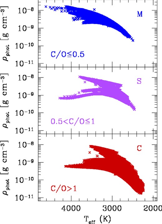
Photospheric gas density (at optical depth τ = 2/3) as a function of the effective temperature for roughly 70 complete TP-AGB evolutionary tracks, spanning the whole range of relevant initial stellar masses, from 0.6 to 6.0 M⊙. The initial chemical composition corresponds to a metallicity Zi = 0.017. Models are grouped according to their surface C/O ratios to represent the chemical classes of M stars (C/O ≤ 0.5), MS-S-SC stars (0.5 < C/O ≤ 1.0) and C stars (C/O >1.0).
Due to the severe uncertainties that still affect our knowledge of stellar convection and stellar winds, both processes are treated in colibri with a parametrized description, mainly in terms of the efficiencies of the third dredge-up and mass loss.
It is common practice to adopt some analytical formula for the mass-loss rate as a function of stellar parameters in stellar evolution models. Doing so, we can then directly compare the modelled HCN abundance as a function of mass loss with observations. However, this practice generates an inconsistency in the present chemo-dynamic models for the wind of TP-AGB stars, as we do not consider dust formation in the HCN formation zone and yet assume dust forms at a specific radius to generate mass loss through radiation pressure on dust grains.
Mass loss is described by assuming that it is caused by two main mechanisms, dominating at different stages. Early in the AGB, when stellar winds are likely related to magneto-acoustic waves operating below the stellar chromosphere, we adopt the semi-empirical relation of Schröder & Cuntz (2005), modified according to Rosenfield et al. (2014). Later in the AGB, when the star enters the dust-driven wind regime, we adopt an exponential form |$\dot{M} \propto \exp ({M^{a} R^{b}})$|, as a function of stellar mass and radius (for more details, see Bedijn 1988; Girardi et al. 2010; Rosenfield et al. 2014), which yields results similar to those obtained with the mass-loss law of Vassiliadis & Wood (1993). The relation was calibrated on a sample of Galactic long-period variables with measured mass-loss rates, pulsation periods, masses, effective temperatures and radii. At any time in the TP-AGB, the actual mass-loss rate is taken as the maximum of the two regimes.
The onset of the third dredge-up is evaluated with envelope integrations at the stage of the post-flash luminosity peak, while its efficiency is computed with analytic fits to the results of full stellar models provided by Karakas, Lattanzio & Pols (2002), as a function of current stellar mass and metallicity. For the metallicity Z = 0.017 considered here, stellar models able to become carbon stars have initial masses Mi ≳ 2.0 M⊙.
Hot-bottom burning in the most massive AGB models (Mi ≳ 4 M⊙) is fully taken into account, with respect to both energetics and nucleosynthesis, by adopting a complete nuclear network (including the proton-proton chains, CNO, NeNa and MgAl cycles) coupled to a diffusive description of stellar convection.
In particular, with colibri we are able to follow in detail the evolution of the surface C/O ratio, which is known to have a dramatic impact on molecular chemistry, opacity and effective temperature every time it crosses the critical region around unity (e.g. Marigo 2002; Marigo, Girardi & Chiosi 2003; Cherchneff 2006; Marigo & Aringer 2009). In turn, the surface C/O ratio plays a paramount role in determining the chemistry of dust in the CSEs of AGB stars (e.g. Ferrarotti & Gail 2006; Nanni et al. 2013).
The high sensitivity of the atmospheric parameters to the surface C/O ratio is illustrated in Fig. 2. The gas pressure and the mass density at the photosphere (at optical depth τ = 2/3) attain maximum values in the neighbourhood of C/O ≃ 1, and then decrease on both sides, corresponding to oxygen-rich (C/O < 1) and carbon-rich models (C/O > 1). The decrease is more pronounced in the models with lower effective temperatures. For HCN, the sharp change in its abundance (relative to that of H2) around C/O ≃ 1 is even more dramatic, and the equilibrium concentration of this carbon-bearing molecule drops by orders of magnitude in the region characterized by C/O < 1, while it rises notably in the opposite region defined by C/O > 1.
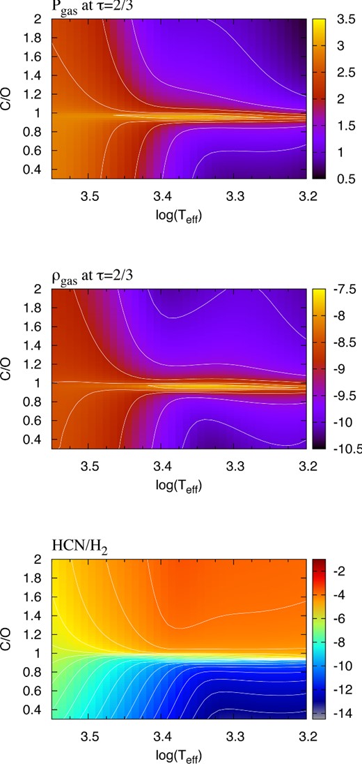
Bi-dimensional map of the logarithms of gas pressure, mass density and equilibrium abundance of HCN relative to molecular hydrogen, as a function of the effective temperature and surface C/O ratio. The C/O ratio is increased from 0.3 to 2.0, in steps of 0.0025, while all other elements are kept constant to their values at the first thermal pulse. Results are obtained with the equilibrium chemistry and opacity routines of the Æsopus code (Marigo & Aringer 2009), applied to a static stellar atmosphere with total stellar mass M = 2 M⊙, initial metallicity Zi = 0.017 and luminosity L = 104 L⊙.
2.1 Chemical definition of M, S and C classes
TP-AGB stars are observationally classified into three groups (M, S and C), mainly based on the molecular absorption features that characterize their spectra. While M stars exhibit prominent molecular bands due to O-bearing molecules (e.g. VO, TiO and H2O), C stars are dominated by strong bands of C-bearing molecules (e.g. CN, HCN and C2). S stars are distinguished by strong ZrO bands in addition to TiO bands typical of M giant spectra. In the past, attempts were made to interpret the phenomenological criteria of spectral classification in terms of stellar parameters: photospheric C/O ratio, effective temperature, gravity and abundances of S-process elements (e.g. Keenan 1954; Keenan & McNeil 1976).
It is generally believed that the C/O ratio is the key factor that drives the spectral dichotomy between M stars (C/O < 1) and C stars (C/O > 1). In this scheme, S stars would be transition objects with C/O ratios within a very narrow range (C/O ≈1). From a theoretical point of view, the increase of the C/O ratio is explained by the recurrent surface enrichment of primary carbon due to the third dredge-up at thermal pulses, which is also generally associated with the increase in the concentrations of heavy elements produced by slow-neutron captures, including Zr (Herwig 2005).
Following the predictions of new model atmospheres, van Eck et al. (2011) recently pointed out that the interval of C/O associated with S stars may be much wider than considered so far, that is 0.5 < C/O ≤1.0. This is essentially because the characteristic ZrO bands observed in the spectra of S stars require that enough free oxygen, not locked in carbon monoxide and other O-bearing molecules, is available.
In the light of the above considerations, in this work we adopt the following operative definition to assign a given TP-AGB stellar model to one of the three chemical classes:
M stars: C/O ≤ 0.5,
S stars: 0.5 < C/O ≤ 1.0,
C stars: C/O > 1.0.
With this definition, the C/O range adopted to characterize the S-star group is meant to gather the sub-classes of MS, S and SC stars (Smith & Lambert 1990). In Fig. 3 we show the evolution of other relevant quantities during the whole TP-AGB phase experienced by a stellar model with initial mass Mi = 2.6 M⊙ and metallicity Zi = 0.017. Following the occurrence of third dredge-up events, this model is expected to experience a complete chemical evolution regulated by the photospheric C/O ratio, starting from the M class, transiting through the S class, and eventually reaching the C class where major mass loss takes place. At the transition to the C-star domain, most of the variables exhibit a notable change in their mean trends, which results in a decrease of the effective temperature and the photospheric density, an increase of the pulsation period and an intensification of the mass-loss rate. The bottom panels present the photospheric concentrations of H2 and HCN, derived with the Æsopus code under the assumption of ICE. As already discussed above, the molecules of hydrogen cyanide are critically affected by the evolution of the C/O ratio. Further modulations in the HCN and H2 abundances are driven by the quasi-periodic occurrence of thermal pulses, clearly recognizable in the oscillating trends on timescales of the inter-pulse period (see also Section 4.4).
![Evolution of several key quantities during the whole TP-AGB evolution of a model with initial mass Mi = 2.6 M⊙ and metallicity Zi = 0.017. From top-left to bottom-right, the 10 panels show: the logarithm of the luminosity [L⊙], the surface C/O ratio, the photospheric density [g cm−3], the effective temperature [K], the pulsation period [d] in the fundamental mode, the logarithm of the mass-loss rate [M⊙ yr−1], the stellar mass [M⊙], the photospheric mean molecular weight [a.m.u.], and the logarithms of the number density [cm−3] of molecular hydrogen H2 and of hydrogen cyanide HCN under the assumption of ICE. All curves are colour-coded as a function of the C/O ratio, namely: C/O ≤ 0.5 in blue, 0.5 <C/O ≤ 1.0 in purple and C/O > 1.0 in red.](https://oup.silverchair-cdn.com/oup/backfile/Content_public/Journal/mnras/456/1/10.1093/mnras/stv2547/2/m_stv2547fig3.jpeg?Expires=1749877888&Signature=ZqFPektxf6yUjuL4JuroZrzFXHGUHCbSvS4f5o27g3xTzpnvCmuop~Nmh6IVyJZRfwzIqLeHy9B9rSjhQI4iJ-kgSwCviuzXZugf9tJszwF4SLGjqUyqh7Dv8GVwK0J-nAcGy~0pwXK1ZkV0iYhwMOM~GlceiElV9JbSQa~EjoXvQWFgnWbg9QZcuJCKJRRKT6iNn0QkCK6v15rwXh1qx2mAiQYSE0xBlkLKRPK4o1GUS9v8tfYVVBWcAmHSdVwvszsGT2mW~f5ZKFKubFzov2TlcJMHlJUeEHazGgt5EwLNuXfQUu8hGVXQlF6F~HBPzA3CWBJE4LRUrjncPCOyog__&Key-Pair-Id=APKAIE5G5CRDK6RD3PGA)
Evolution of several key quantities during the whole TP-AGB evolution of a model with initial mass Mi = 2.6 M⊙ and metallicity Zi = 0.017. From top-left to bottom-right, the 10 panels show: the logarithm of the luminosity [L⊙], the surface C/O ratio, the photospheric density [g cm−3], the effective temperature [K], the pulsation period [d] in the fundamental mode, the logarithm of the mass-loss rate [M⊙ yr−1], the stellar mass [M⊙], the photospheric mean molecular weight [a.m.u.], and the logarithms of the number density [cm−3] of molecular hydrogen H2 and of hydrogen cyanide HCN under the assumption of ICE. All curves are colour-coded as a function of the C/O ratio, namely: C/O ≤ 0.5 in blue, 0.5 <C/O ≤ 1.0 in purple and C/O > 1.0 in red.
3 CHEMO-DYNAMIC EVOLUTION OF THE INNER CIRCUMSTELLAR ENVELOPE
Several theoretical studies have clearly pointed out that the strong pulsations experienced by AGB stars cause periodic shock waves to emerge from sub-photospheric regions, from where they propagate outward through the stellar atmosphere and the CSE (Wood 1979; Willson & Hill 1979; Fox & Wood 1985; Bertschinger & Chevalier 1985; Bowen 1988). To model the shock dynamics and the non-equilibrium chemistry across the circumstellar region that extends from the photosphere at r = 1R to r = 5R, which we refer to as the inner wind, we adopt the basic scheme developed in Cherchneff et al. (1992) and Willacy & Cherchneff (1998).
Below we will recall the basic ingredients and introduce the main modifications with respect to the original prescriptions. We will adopt the standard notation that marks with the subscripts 1 and 2 the gas conditions in front of (pre-shock) and behind the shock (post-shock), respectively. The functional forms for time-averaged radial temperature and density profiles of the pre-shock gas are the same as in Cherchneff et al. (1992), and we refer to that paper for many technical details.
3.1 The time-averaged pre-shock temperature
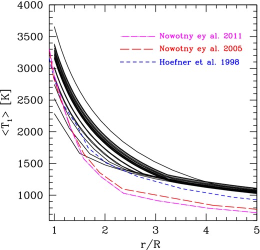
Radial profile of the average pre-shock temperature of the gas, across a distance from r = 1R up to r = 5R. Each solid line corresponds to the temperature structure at the quiescent luminosity just preceding each thermal pulse during the whole TP-AGB evolution of a (Mi = 2.6 M⊙, Zi = 0.017) model computed with the colibri code. For comparison, we overplot three temperature profiles taken from detailed hydrodynamic models, averaged over the pulsation phases (Höfner et al. 1998; Nowotny et al. 2005, 2011).
For carbon-rich models (C/O >1), we take p = 1, which is a reasonable assumption for amorphous carbon grains in the relevant spectral region 1–30μ, and Tcond = 1500 K (Cherchneff, Barker & Tielens 1991; Jager, Mutschke & Henning 1998). These values for p and Tcond lead to rcond rather close to the star (rcond/R ≲ 2–4) for carbon stars with intense mass loss, in line with detailed dust models and observational indications (e.g. Ferrarotti & Gail 2006; Nanni et al. 2013; Karovicova et al. 2013).
For oxygen-rich models (C/O <1), the situation is more complex and uncertain, since p is shown to change significantly, i.e. from 2 to −1 when passing from iron-rich olivine grains to forsterite (Dorschner et al. 1995; Jäger et al. 2003; Andersen 2007). We were not able to identify a suitable unique prescription in the form of equation (2) that performs well for all TP-AGB models. Empirically, we find that the relation rcond/R = 0.24 exp (1.87/M) + 0.027M + 2.68 (where M is the current stellar mass) leads to density and temperature profiles suitable for HCN chemistry in O-rich models. We get typical values rcond/R ≲ 3–4 in line with interferometric observations (Wittkowski et al. 2007; Karovicova et al. 2011; Norris et al. 2012) and theoretical studies (Bladh et al. 2013, 2015). We plan to improve the above prescription with a more physical basis in follow-up studies.
We also remark that the issue of dust formation is beyond the purpose of this initial work, and the related quantities (Tcond and rcond) are relevant here only for the definition of the boundary conditions of the dynamic model (see Section 3.3).
Fig. 4 presents the predicted temperature gradients across the CSE of a stellar model during the TP-AGB phase, each line corresponding to the stage just prior to the occurrence of a thermal pulse. The temporal sequence is characterized by the decrease of the effective temperature, which coincides with the gas temperature at r = 1R. The flattening of the slope in the 〈T1(r)〉 relations for r > rcond is particularly evident for the coolest tracks, which are for the latest stages on the TP-AGB characterized by strong mass loss. For comparison, we plot a few curves that are the results of detailed dynamic models for pulsating C-rich atmospheres, all corresponding to an effective temperature Teff = 2600 K (Höfner et al. 1998; Nowotny et al. 2005, 2011). Indeed, the average trends are well recovered by our models, though they tend to be shifted at somewhat higher T. In this respect, one should also note that the input stellar parameters are not the same, e.g. most of our pre-flash TP-AGB stages correspond to effective temperatures Teff > 2600 K.
3.2 The time-averaged pre-shock density
The description of the time-averaged pre-shock gas density is that presented by Cherchneff et al. (1992) following the formalism first introduced by Willson & Bowen (1986) based on dynamic models for periodically shocked atmospheres. Three wind regions are considered: (1) the static region, which is controlled but has a static scale height; (2) the pulsation-shocked region, which is controlled by an extended scale height due to shock activity and (3) the wind region where the wind fully develops once dust has formed. The equation of momentum conservation is integrated over radial distance by assuming spherical symmetry.
The characteristic scale height H(r) and the reference point at r = r0 depend on the local mechanical conditions across the pulsating atmosphere. Let us denote with rs,0 the radius at which the first shock develops.
3.2.1 The static region
3.2.2 The pulsation-shocked region
We note that, as long as γshock < 1 (see Fig. 6), Hdyn(r) > H0(r), which implies that in the shocked region the average density is higher than otherwise predicted under the assumption of hydrostatic equilibrium. This is a key point for the non-equilibrium molecular chemistry that is active in that region.
3.2.3 The wind region
We assume that at the dust condensation radius rcond, the stellar wind starts to develop. The driver is thought to be the radiative acceleration of dust particles with subsequent collisional transfer of momentum from the grains to the surrounding gas (Gustafsson & Höfner 2004).
Fig. 5 illustrates a temporal sequence of pre-shock density profiles, referring to the same TP-AGB evolution as in Fig. 4. Calculations were carried out with rs,0 = 1R, so that the CSE does not include a static region and the pulsation-shocked zone starts from the photosphere. Each curve shows a clear change in the average slope, which becomes flatter at the condensation radius from where the stationary wind regime is assumed to start.

For comparison, the results from detailed models of pulsating atmospheres are also shown. A nice agreement is found in most cases. In particular, the radial decline of the density predicted by the stationary wind condition compares surprisingly well with the phase-averaged slopes of the detailed shocked-atmosphere models, just over the distances where dust is expected to be forming efficiently.
3.3 Boundary conditions for the density and the initial shock amplitude
The parameter γshock is a critical quantity since it determines the dynamic scale height of the density across the shock-extended region (see equation 5). Cherchneff et al. (1992) adopted γshock = 0.89 in their dynamic model for the carbon-rich star IRC+10216, following considerations about the location of the shock formation radius rs,0.
Since then, to our knowledge, all the works in the literature based on the Cherchneff et al. (1992) formalism have always kept the same value, γshock = 0.89, even if they analyse a different object, such as the S star χ Cig, or the oxygen-rich stars TX Cam and IK Tau, or they adopt different prescriptions for other parameters, such as the shock formation radius rs,0, the initial shock strength Δυ0, the pulsation period, etc. (Willacy & Cherchneff 1998; Duari & Hatchell 2000; Cau 2002; Cherchneff 2006; Agúndez & Cernicharo 2006; Cherchneff 2011, 2012; Agúndez et al. 2012; Duari et al. 1999).
With equation (10), we assume that the sonic point coincides with the condensation radius rcond, which is a reasonable condition as it is generally thought that radiation on dust grains is the main process driving supersonic outflows in AGB stars (Lamers & Cassinelli 1999).
In summary, the boundary condition for the density, given by equation (10), translates into a function of the parameter γshock, which is eventually found with a standard numerical iterative technique. Once γshock is known, we can obtain the corresponding value for the initial shock amplitude Δυ0 = γshock × υe(rs,0), where the escape velocity is evaluated at the shock formation radius. In this way, we consistently couple two key parameters of the dynamic model, γshock and Δυ0, which are often kept as independent input quantities in the works cited above.
Fig. 6 shows the evolution of Δυ0 (assuming that rs,0 = R) for a representative sample of models with different initial stellar masses over the entire TP-AGB evolution. The initial shock amplitude Δυ0 is found to progressively decrease during the TP-AGB evolution. This finding is in line with the general trends of detailed calculations of periodically shocked atmospheres (Bowen 1988), in which Δυ0 is predicted to reduce with increasing pulsation period (see his table 6) and decreasing effective temperature (see his table 9), a trend that also happens as the TP-AGB evolution proceeds.
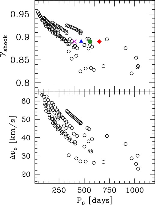
Evolution of the dynamic parameters γshock (top panel) and maximum shock amplitude Δυ0 (bottom panel) as a function of the pulsation period in the fundamental mode. Predictions for the whole TP-AGB evolution of a few selected models of different initial masses (Mi = 1–4 M⊙; empty circles) are shown. Note the significant dispersion for γshock, extending well above and below the constant value of 0.89 assumed in several existing models (referenced in the text), dealing with different stars, such as IRC+10216 (square), TX Cam (circle), IK Tau (triangle) and χ Cyg (cross).
Once Δυ0 at r = rs,0 is singled out for each combination of the stellar parameters, the weakening of the shock strength Δυ(r) at increasing r is described according to equation (8). Fig. 7 shows the predicted damping of Δυ(r) as a function of the pre-shock density across the CSE of a low-mass TP-AGB stellar model with initial mass Mi = 1.4 M⊙ and metallicity Zi = 0.017. Interestingly, at distances around r/R ≃ 3, the tracks enter the region of the (ρ1, Δυ) space that seems to provide the suitable conditions for the formation of the observed Fe ii and [Fe ii] peak line fluxes and line ratios in a sample of Mira stars (Richter & Wood 2001; Richter et al. 2003).
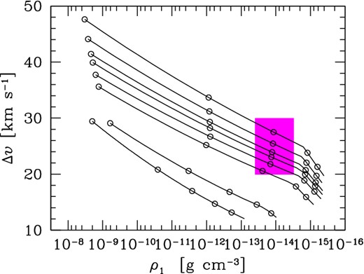
Evolution of the shock amplitude Δυ as a function of the quiescent pre-shock density 〈ρ1(r)〉 as the shock propagates across the CSE, during the whole TP-AGB evolution of a star with initial mass Mi = 1.4 and metallicity Zi = 0.017. Each track corresponds to the stellar parameters just preceding a thermal pulse (the temporal sequence of thermal pulses proceeds from top to bottom). The hatched region in magenta defines the suitable region of the Δυ–〈ρ1(r)〉 plane where both normalized peak fluxes of the permitted and forbidden Fe ii emission lines fit the observed data for a sample of Mira stars, following the analysis of Richter et al. (2003) and Richter & Wood (2001). The empty circles mark the positions through the CSE from r/R = 1 to r/R = 5 in steps of Δ(r/R) = 1.
3.4 The gas outflow velocity
Another quantity of interest is the average radial increase of the gas outflow velocity, υgas,1, which is calculated with the Parker theory of stellar winds (Parker 1965) and following the prescriptions of Cherchneff et al. (1992), which take into account the shocks and radiation pressure on dust. The condensation radius is assumed to coincide with the Parker radius, where the gas velocity equals the isothermal speed of sound given by equation (11).
The Parker solution for the average gas velocity is illustrated in Fig. 8, which shows the radial profile of υgas,1 for three TP-AGB models with different photospheric C/O ratios (0.39, 0.87 and 1.44), which may be considered representative of the chemical classes M, S and C. Starting from the stellar photosphere, the outflow is initially subsonic, with low velocities typically ≲ 1 − 2 km s−1. The isothermal sound velocity (υs,T ≃ 2.0–2.2 km s−1) is reached at the Parker radius (equal to rcond by construction), which appears to be located in the range ≈2.0–3.5R. Note that for the C star model, characterized by the longest period and highest mass-loss rate, rP sits closer to the star than in the other two M and S models. Beyond the sonic point, the outflow is accelerated due to radiation pressure on dust grains.

Gas outflow velocity υgas,1 as a function of the radial distance from the stellar centre. The curves correspond to the pre-flash quiescent stages of the second, 11th and 17th thermal pulses, experienced by the TP-AGB evolutionary model with initial mass Mi = 2.6 M⊙ and metallicity Zi = 0.017. For the three cases, the filled symbols (circle, square and triangle) mark the corresponding positions of the sonic point, where the gas velocity equals the isothermal speed of sound. See the text for more details.
Note that a careful consideration of the dust issue is beyond the scope of this initial work. Knowing υgas,1 has mainly a practical relevance in the present context, since we use it for defining the radial grid of mesh points over which the integrations of the shock dynamics and non-equilibrium chemistry are performed, as described in Section 3.7. The crosses on the curves mark the positions reached after one pulsation period by a gas parcel that is moving outward with a velocity υgas,1(r). Over the distance from r = 1R to r = 5R, we typically deal with a few tens to several tens of radial mesh points for each CSE.
3.5 Pulsation-induced shocks
The time-dependent structure of the shocked atmosphere and inner wind have been modelled according to the works of Willacy & Cherchneff (1998), Duari et al. (1999) and Cherchneff (2006, 2011, 2012). These studies apply the semi-analytical formalism of Bertschinger & Chevalier (1985), where the shocked gas initially cools by emitting radiation in a thin layer just after the shock front. Then, the gas enters the post-shock deceleration region where its velocity decreases under the action of the stellar gravity, before being shocked again. Three main assumptions are adopted.
First, the Lagrangian trajectory of any fixed fluid element is strictly periodic with zero mass loss. This is reasonable in the inner CSE regions, where the gas remains gravitationally bound to the star (Gustafsson & Höfner 2004). Periodicity also means that, at any time, after being accelerated up to a maximum height above the shock formation layer, the gas element is decelerated downward until it recovers its original unperturbed position. With a mass flux moving outward with an unperturbed velocity υgas,1, this is not exactly true, and the particle orbits are not exactly closed. However, we have verified that, after one pulsation period, the radial displacement, Δr = υgas,1 × P, of the fluid element with respect to the original position r remains quite small in most cases, the relative deviation Δr/r remaining typically below a few 10−1.
Secondly, the shock waves are radiative, so that the gas quickly cools by emission of radiation in a thin region behind the shock front. The post-shock values T2 and ρ2 are fixed by the Rankine–Hugoniot conditions (Nieuwenhuijzen et al. 1993).
Thirdly, during the post-shock deceleration phase, the effect of the interaction between the gas and radiation, hence, of possible radiative losses, is implicitly taken into consideration by introducing an arbitrary effective adiabatic exponent |$\gamma _{\rm ad}^{\rm eff}$|. In fact, the adiabatic exponent can significantly deviate from the classical predictions (e.g. γad = 1.4 for a diatomic perfect gas), when otherwise neglected non-ideal phenomena, such as ionization, dissociation of molecules and radiation pressure, are suitably taken into account. In this respect, a thorough analysis is provided by Nieuwenhuijzen et al. (1993). Therefore, in view of a more general description, in place of the classical adiabatic index γad, we opt to use |$\gamma _{\rm ad}^{\rm eff}$| as a free parameter to be inferred from observations. An ample discussion about |$\gamma _{\rm ad}^{\rm eff}$| and its calibration is given in Section 4.2.1.
Following Bertschinger & Chevalier (1985), for a given combination of stellar parameters (M, Teff, R, P, μ, T1, ρ1), all the properties of the shock that emerges at the radius r = rs are completely determined once one specifies two parameters, namely, the effective adiabatic exponent |$\gamma _{\rm ad}^{\rm eff}$| and the pre-shock Mach number M1. An example application of the shock model is presented and discussed in Section 3.7.
3.6 Molecular chemistry
The evolution of the gas chemistry through the inner zone of the CSE is followed for 78 species (atoms and molecules) using a chemo-kinetic network that includes 389 reactions. The network is essentially the same as the one as set up by Cherchneff (2012) in her study of the carbon star IRC+10216. It includes termolecular, collisional/thermal fragmentation, neutral–neutral and radiative association reactions and their reverse paths. The chemical species under consideration are listed in Table 1.
Molecular species included in the chemical network taken from Cherchneff (2012). Involved chemical elements are: H, He, C, N, O, F, Na, Mg, Al, Si, P, S, Cl, K and Fe.
| O-bearing molecules |
| OH, H2O, CO, HCO, O2, SiO, SO, |
| NO, CO2, MgO, FeO, H2OH |
| C-bearing molecules |
| CN, HCN, C2H2, C2H3, CH2, C2, |
| CS, SiC, CH, CH3, HCP, CP, C3, |
| C2H, C4H3, C4H2, Si2C2, C3H2, |
| C3H3, C4H4, C6H5, C6H6, Si2C2 |
| Other molecules |
| H2, NH, N2, NH2, NH3, PH, P2, |
| PN, SiN, SH, H2S, MgH, MgS, Mg2, |
| FeH, FeS, Fe2, HF, F2, ClF, AlH, |
| AlCl, NaH, NaCl, HCl, Cl2, KH, KCl |
The integration in time of the system of stiff ordinary coupled differential equations is carried out with the publicly available chemistry package krome (Grassi et al. 2014).1 For comparison, we will explore also the predictions for the molecular chemistry under the assumption of ICE, computed with the Æsopus code (Marigo & Aringer 2009), which includes more than 500 molecular and 300 atomic species.
3.7 Chemo-dynamic integrations
At any stage along the TP-AGB, the stellar parameters at the photosphere (r = R) predicted by colibri, together with the ICE chemical abundances of atoms and molecules provided by Æsopus, are used as initial conditions for the chemo-dynamic integrations of the inner CSE. Beyond the photosphere, we adopt essentially the same Lagrangian formalism as described by Willacy & Cherchneff (1998), Duari et al. (1999), Cau (2002) and Cherchneff (2006, 2011, 2012), to whom we refer for all the details. A few important modifications are introduced.
At any fixed value of the radial distance r, the chemistry of a gas parcel is solved over two pulsation periods, which is enough to check for the periodicity of thermodynamic and abundance parameters. The molecular concentrations after two pulsation cycles at r are then used as input for the next two chemical integrations at r + Δr, once they have been rescaled to the new pre-shock gas density. We take the incremental step Δr = P × υgas,1(r), that is the distance travelled by the gas element during one pulsation period with the gas velocity υgas,1, computed as detailed in Section 3.4.
Each of the two integrations includes both (1) the very fast chemistry of the chemical cooling layer introduced by Willacy & Cherchneff (1998) and (2) the prolonged chemistry activity during the post-shock hydrodynamic cooling. In both regimes, the non-equilibrium chemistry is solved with the krome routines.
We note that by applying a Lagrangian formalism over the radial extension of the inner CSE, it is possible to obtain an Eulerian-type profile of the chemical species, which can eventually be compared with the measured concentrations.
In this initial study, we do not consider any processes of dust condensation and growth, which we postpone to follow-up works, and we focus on the hydrogen cyanide molecule, the formation of which, observational evidence suggests, is not affected by dust grain formation (Schöier et al. 2013).
For illustrative purposes, Fig. 9 shows the solution for the chemo-dynamic structure of an AGB pulsating stellar atmosphere traversed by periodic shocks, over two pulsation periods. In the Lagrangian framework, the variations of the fluid variables (radius, velocity, density, temperature, mean molecular weight and molecular hydrogen abundance) are plotted as a function of the pulsation phase along the decelerating particle trajectory.
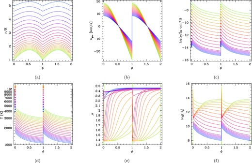
Shocked gas properties during the adiabatic expansion, as a function of the phase over two pulsation cycles, caused by periodic shock propagation. In each panel, the bunch of lines (with colours gradually changing along the sequence green–red–blue) corresponds to a grid of shocks that develop at increasing radial distance from r = 1R to r = 5R, in steps of Δr = υgas,1 × P. From top-left to bottom-right, the six panels show: (a) the Lagrangian trajectories of a gas parcel, (b) the gas velocity with respect to the stellar rest frame, (c) the mass density and (d) the temperature (the shock-front values determined by the Rankine–Hugoniot conditions are indicated by filled circles), (e) the mean molecular weight (in atomic mass units) and (f) the logarithm of the number density of molecular hydrogen (in cgs units). The first shock is assumed to emerge at rs,0 = 1R. The effective adiabatic exponent is taken to be |$\gamma _{\rm ad}^{\rm eff} = 1.1$|. Our dynamic model predicts the initial shock amplitude Δυ0 = 47 km s−1 at rs,0 = 1R, the initial pre-shock Mach number M1 = 10.447 and the dynamic parameter γshock = 0.896. The shocked atmosphere corresponds to the quiescent stage just preceding the 13th thermal pulse of a carbon-rich TP-AGB model, with current mass M = 2.311 M⊙ (initial mass Mi = 2.6 M⊙), effective temperature Teff = 3020 K, luminosity log (L/L⊙) = 3.899, pulsation period in the fundamental mode P0 = 301 d, photospheric C/O = 1.06, mass-loss rate |$\dot{M} = 4.34 \times 10^{-7}\,{\rm M}_{{{\odot }}}\,{\rm yr}^{-1}$| and dust condensation radius rcond = 2.78R.
The outward propagation of the shock is followed from its first appearance at rs,0 = 1R up to r = 5R, according to a discrete grid of radial meshes. The reference system is the stellar rest frame, in which the radial distance is measured from the centre of the star under the assumption of spherical symmetry. Positive gas velocities correspond to the initial upward displacement of the gas parcel driven by the pressure forces, while negative gas velocities describe the subsequent downward motion due to the gravitational pull, back to the original location.
During the post-shock relaxation, both the mass density and the temperature are expected to decrease until ϕ = 1, when the fluid element recovers its initial values, experiences the next shock and the cycle repeats itself.
It is also interesting to examine the evolution of the mean molecular weight μ of the shocked gas. For shocks that emerge closer to the star (r < 3R), μ is seen to increase with the pulsation phase ϕ, due to the progressive increment of the molecular concentrations relative to the atomic abundances, which instead dominate at ϕ ≃ 0 (where μ ≈ 1.35–1.40). This is explained by the decrease of the temperature during the post-shock gas expansion. At larger distances (r > 3R), the temperature at the beginning of the dynamic relaxation is low and the gas is already mainly in molecular form at ϕ ≃ 0. In these models, the mean molecular weight remains almost constant during the whole pulsation cycle, attaining values that are typical of a gas chemistry dominated by molecular hydrogen and carbon monoxide (μ ≈ 2.40–2.45).
4 CSE ABUNDANCES OF HYDROGEN CYANIDE
We follow the chemistry of several molecular species in our model (see Table 1). However, the discussion of all trends and results is not addressed in this initial paper, and we postpone a thorough analysis to follow-up works.
As a first application, we decided to focus on the hydrogen cyanide molecule for two main reasons. First, we can rely on plentiful data of HCN concentrations measured in CSEs of AGB stars, so that a statistical study is now feasible. Secondly, the HCN abundances have proved an excellent tool for calibrating the dynamics of the inner CSEs, without running into the uncertainties and complications of the growth of dust grains, which, in fact, does not affect the chemistry of the HCN molecule.
Indeed, the HCN molecule has been detected in AGB CSEs of all chemical types (Bieging, Shaked & Gensheimer 2000; Marvel 2005; Muller et al. 2008; Schöier et al. 2013). Using a detailed radiative transfer model, Schöier et al. (2013) have recently derived the circumstellar HCN abundances for a large sample of AGB stars, spanning a wide range of properties, mainly in terms of chemical types, mass-loss rates and expansion velocities.
This sample notably enlarges the observed range of the parameter space, and therefore it provides a robust statistical test for chemical models that aim at investigating the molecular chemistry in the inner CSE regions close to the photospheres of long-period variables.
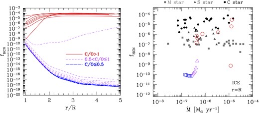
The main result of the analysis of Schöier et al. (2013) is the strong dependence of the HCN abundances on the photospheric C/O ratio, with a clear trend of increasing HCN/H2 when moving along the spectral sequence of M-S-C. This property is shown in Fig. 10, where the estimated HCN abundances are plotted as a function of the mass-loss rate for the three chemical types.
![HCN fractional abundances relative to molecular hydrogen, f(HCN) = n(HCN)/[n(H2 + 0.5n(H)], as a function of the mass-loss rate for a sample of 69 AGB stars that include M stars (squares), S stars (triangles) and C stars (circles). HCN data are obtained from a multi-transition survey of HCN (sub-)millimetre line emission carried out by Schöier et al. (2013). Typical error bars in the measurements of f(HCN) and $\dot{M}$ are shown. Well-known stars are marked as in the top legend.](https://oup.silverchair-cdn.com/oup/backfile/Content_public/Journal/mnras/456/1/10.1093/mnras/stv2547/2/m_stv2547fig10.jpeg?Expires=1749877888&Signature=SLTawEGWIhIC2ZDDghZBHuC00NBFln-oH2T54NjxvjcXr2Don~l-MM4vRTrjnFlk~AP5fM-BA59qGiMltYnzWktiM6Vts-znD7trPKKaytgN5~Ss0MBtcHxW-Wy-hPtEZFxHsMepxMTeBFLs73uIqFnN1Ztxyh7Sg80rH24gpIF8ei2Eifcq3M~xqvD2lTa06uYSNJDSLBVdPPQyxUITVvi29cMCYEv5aU8SN49Nwi-Yght13-IEZLlW7F-7XB5ZMmP5UjXKY~K4fTj1Sb3JjJyepI4nkcaMH-1V1IMAL8bamUEH9fL9ez-nqq~gKHg9Ypx2m-DofnH9PtfHQ1-AEQ__&Key-Pair-Id=APKAIE5G5CRDK6RD3PGA)
HCN fractional abundances relative to molecular hydrogen, f(HCN) = n(HCN)/[n(H2 + 0.5n(H)], as a function of the mass-loss rate for a sample of 69 AGB stars that include M stars (squares), S stars (triangles) and C stars (circles). HCN data are obtained from a multi-transition survey of HCN (sub-)millimetre line emission carried out by Schöier et al. (2013). Typical error bars in the measurements of f(HCN) and |$\dot{M}$| are shown. Well-known stars are marked as in the top legend.
The authors also concluded that the observed sensitivity of the HCN abundance on C/O is in sharp contrast with shock-induced chemistry models, in which the predicted HCN abundances are essentially insensitive to the stellar chemical type (Cherchneff 2006). It should be noted that the results of those shock-induced chemistry models for the HCN dependence on the C/O ratio were obtained for a single combination of stellar parameters (M = 0.65 M⊙, R = 280 R⊙ and P = 557 d), and a fixed choice of dynamic parameters (rs,0 = 1R, γshock = 0.89 and Δυ0 = 25 km s−1). Furthermore, the results of Cherchneff (2006) for HCN might be obsolete following the significant revision of the chemical network carried out by Cherchneff (2011, 2012). This is the main reason why we choose to use this later revised network in the present study.
In this work, we aim at extending shock-chemistry analysis over a wide range of physical parameters, most of which are extracted directly from stellar evolutionary calculations for the TP-AGB phase.
In the following, we analyse the predictions for HCN abundances in the inner CSEs of TP-AGB stars, both under the assumption of ICE and for non-equilibrium chemistry applied to periodic shocks. Thus, we will test the results for a TP-AGB evolutionary track with initial mass Mi = 2.6 M⊙ and metallicity Zi = 0.017, computed with the colibri code (Marigo et al. 2013). This model is predicted to experience the third dredge-up and to become a carbon star attaining a final surface C/O = 1.55. A summary of the evolutionary properties along the TP-AGB phase is given Section 2, and illustrated in Fig. 3. Calculations for other TP-AGB models with different initial masses will be also presented.
In general, we choose to compare observations to our fHCN abundances in the range 3 < r/R < 5 because at those distances the HCN chemistry is frozen out. At the same time, these radii are much smaller than the typical e-folding radius for HCN inferred from observations, so that our predictions are directly comparable with the initial abundances f0, as reported by Schöier et al. (2013, see their section 3.4).
4.1 Equilibrium chemistry
Several studies have already demonstrated that the chemistry that controls the inner wind of AGB stars is not at equilibrium owing to the presence of shocks (e.g. Willacy & Cherchneff 1998; Duari et al. 1999; Cherchneff 2006, 2012), but as a first test, we consider ICE, which we compute with the Æsopus code (Marigo & Aringer 2009). Fig. 11 shows the predicted abundances of HCN relative to molecular hydrogen as a function of the distance from the stellar centre, for the reference model with initial mass Mi = 2.6 M⊙ and metallicity Zi = 0.017.
Fractional abundance fHCN under the assumption of ICE with the Æsopus code (Marigo & Aringer 2009), corresponding to our reference model with initial mass Mi = 2.6 M⊙ and metallicity Zi = 0.017, which is expected to experience 20 thermal pulses evolving along the chemical sequence M-S-C due to the third dredge-up. For each radius, chemistry predictions are shown after the completion of two consecutive pulsation cycles. Left-hand panel: Radial profiles of HCN/H2 concentrations for r = 1–5R CSE. Each line corresponds to the stellar evolutionary stage just preceding a thermal pulse. Right-hand panel: Fractional abundances fHCN at the photosphere (empty symbols) under the ICE assumption, as a function of the mass-loss rate during the entire TP-AGB evolution. Models are denoted with blue squares for C/O ≤0.5, purple triangles for 0.5 < C/O ≤1.0 and red circles for C/O >1.0. Observed data are the same as in Fig. 10.
As expected, the equilibrium abundance of HCN is remarkably sensitive to the C/O ratio. As long as the star remains oxygen-rich with C/O < 0.9, the HCN concentration is quite low and decreases significantly while moving away from the stellar photosphere (left-hand panel of Fig. 11). Correspondingly, at any radial distance, the predicted ICE abundances are lower than the measured ones for M stars by several orders of magnitudes. The comparison with the photospheric abundances for the equilibrium chemistry (right-hand panel of Fig. 11) underlines that even in the most favourable conditions of high gas density, the predicted fHCN for M and S stars (≃10−10) is already much lower than the observed data by a few orders of magnitude.
As the C/O ratio increases due to the third dredge-up events and enters the critical narrow range regime 0.9 ≤ C/O <1.0, the equilibrium abundances of HCN abruptly rise, spanning a remarkably wide range. However, even the highest values (HCN/H2 ≃ 10−9 for C/O ≃ 0.967 at the 12th thermal pulse) keep well below the observed median concentration for S stars (HCN/H2 ≃ 7 × 10⁻⁷).
Eventually, as soon as the star becomes carbon rich (C/O >1), a remarkable increase of the HCN abundances (by several orders of magnitude) takes place and the predicted equilibrium abundances reach values that appear to be consistent with the measured data for carbon stars, starting from r/R > 2.
In view of the above, we may conclude that the ICE chemistry is not suitable for explaining the observations of HCN in the CSEs of AGB stars with different chemical types, as already mentioned by Cherchneff (2006).
4.2 Non-equilibrium chemistry: dependence on main shock parameters
In the following, we will analyse the HCN abundances predicted by calculations of non-equilibrium chemistry regulated by pulsation-induced shocks, which propagate across the CSE.
In particular, we will investigate the dependence of the results on two fundamental parameters, namely the shock formation radius rs,0 and the effective adiabatic index |$\gamma _{\rm ad}^{\rm eff}$| (see Section 3.5). In fact, both quantities control the excursions in density and temperature experienced by a gas parcel shocked by pulsation.
4.2.1 The effective adiabatic index
In the shock formalism adopted here (Bertschinger & Chevalier 1985; Willacy & Cherchneff 1998), |$\gamma _{\rm ad}^{\rm eff}$| is the key input parameter, which, together with the pre-shock Mach number M1, determines the temperature Tc and the density ρc at the top of the deceleration region, from where the hydrodynamic expansion phase starts. In general, the higher |$\gamma _{\rm ad}^{\rm eff}$|, the larger Tc and ρc are attained. They correspond to the pulsation phase ϕ = 0 in panels (c) and (d) of Fig. 9.
We have explored a few choices of the effective adiabatic index, namely |$\gamma _{\rm ad}^{\rm eff}= 1.4, 1.2, 1.1$| and 1.01. The highest value was often adopted in previous studies (e.g. Cau 2002, and references therein). The results are illustrated in the four panels of Fig. 12, corresponding to our reference TP-AGB stellar model. A few considerations can be drawn.
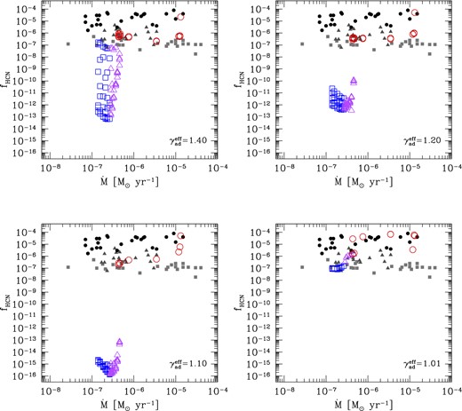
Comparison between observed fractional abundances fHCN and predictions of shock-chemistry models on varying the effective adiabatic index |$\gamma _{\rm ad}^{\rm eff}$|. In all calculations, we assume rs,0/R = 1. Open symbols correspond to predicted abundances over the entire TP-AGB evolution of a model with initial mass Mi = 2.6 M⊙ and metallicity Zi = 0.017, which is expected to evolve along the chemical sequence M-S-C due to the third dredge-up. At the given mass-loss rate, the model abundances are shown across the distance range r = 3–5R. Note the striking agreement with the data for shock models that assume |$\gamma _{\rm ad}^{\rm eff}=1.01$|, which points to a prevalent isothermal character of the shocks in the inner CSE.
For all three values |$\gamma _{\rm ad}^{\rm eff}> 1$|, the HCN concentrations are always below the measured data at any value of the photospheric C/O ratio. The theoretical underestimation is more pronounced for the M and S stars, amounting to several orders of magnitudes. In all cases, the radial profile of HCN abundance is characterized by large variations, which explain the sizable scatter of the predictions over a distance range 3 ≲ r/R ≲ 5 for a given mass-loss rate. A significant improvement in the comparison of the model data is obtained by lowering the effective adiabatic index to |$\gamma _{\rm ad}^{\rm eff}\simeq 1$|.
We note that lowering |$\gamma _{\rm ad}^{\rm eff}$| from 1.1 to 1.01 produces a large increase of fHCN for the M and S models. Such a dramatic change is related to the evolution of temperature and density during the post-shock relaxation, which affects the HCN formation through the H2/H ratio (see the extensive discussion in Section 4.3). When |$\gamma _{\rm ad}^{\rm eff}$| is relatively high, the higher temperature at early phases destroys/prevents the formation of H2, whereas at later phases (when the temperature would be suitable for H2 formation), the rate of H2 formation is low because of the low density reached during the post-shock relaxation. When |$\gamma _{\rm ad}^{\rm eff}$| is close to 1 (radiative shocks), the cooling is so efficient that the temperature is suitable for H2 formation at almost all phases.
By adopting |$\gamma _{\rm ad}^{\rm eff} \simeq 1$|, the predicted HCN abundances over the 3 ≲ r/R ≲ 5 radial distance and during the TP-AGB evolution match the observed data points very well. In particular, the model recovers the observed stratification of the HCN concentrations that are seen to increase, on average, when moving along the chemical sequence of M, S and C stars. This result supports the empirical fact that the photospheric C/O ratio is one of the major factors determining the CSE chemistry of HCN, and is at variance with previous conclusions (Cherchneff 2006).
Moreover, we note that for |$\gamma _{\rm ad}^{\rm eff}\simeq 1$|, the theoretical dispersion of the HCN abundances becomes quite narrow at varying radial distance in the 3 ≲ r/R ≲ 5 interval. This finding means that the shock chemistry for HCN tends to freeze out at increasing distance and is consistent with the observational evidence that the HCN concentrations attain typical values, which do not change dramatically, especially within a given chemical class of mass-losing AGB stars.
In conclusion, our tests suggest that to explain the CSE concentrations of HCN with non-equilibrium chemistry, the pulsation-induced shocks in the inner zone around AGB stars should be described by a low value of the effective adiabatic index, that is |$\gamma _{\rm ad}^{\rm eff} \simeq 1$|.
It is quite interesting to interpret this finding in terms of physical implications. If radiative processes are not important, |$\gamma _{\rm ad}^{\rm eff}$| is determined by the thermodynamic equilibrium of the gas. For instance, for a gas mostly consisting of hydrogen, |$\gamma _{\rm ad}^{\rm eff}=5/3$| for atomic hydrogen, |$\gamma _{\rm ad}^{\rm eff}=1.4$| for molecular hydrogen without vibrational degrees and |$\gamma _{\rm ad}^{\rm eff}=9/7$| for molecular hydrogen with vibrations excited (Zel'dovich & Raizer 1966).
Deviations towards lower values for |$\gamma _{\rm ad}^{\rm eff}$| may actually occur if radiative processes become significant in the thermal relaxation behind the propagating shock waves, so that the assumption of thermodynamic equilibrium cannot be safely applied.
An indication that this may indeed be the case for Mira variables was derived by Bertschinger & Chevalier (1985) from their model fits to the observed CO Δυ = 3 excitation temperature as a function of the phase for four stars (o Ceti, T Cep, χ Cyg and R Cas). In all cases, they obtained |$\gamma _{\rm ad}^{\rm eff}\simeq 1.1$|.
In this context, Woitke (1997) provided a thorough discussion about the character of the thermal relaxation behind the shock, which is critically affected by the timescale necessary for the gas to radiate away its excess of internal energy dissipated by the shock. In brief, the thermal behaviour of the gas in the CSEs of pulsating stars depends on the comparison between the radiative cooling timescale τcool and the stellar pulsation period P:
If τcool ≳ P then the gas cannot radiate away the energy dissipated by one shock within one pulsation period, and therefore, it cools adiabatically.
If τcool ≪ P, the gas quickly relaxes to radiative equilibrium behind the shock before the next shock wave hits it, so that the dominant character is that of an isothermal shock.
On a temperature–density diagram, one can conveniently define a critical cooling track along which the maximum radiative cooling time is τcool = 1 yr, considering 1 yr as a typical period of a Mira variable. Two such critical lines are drawn in Fig. 13 according to the computations of Woitke (1997), for two choices of the radiation temperature, i.e. Trad = 0 K (dashed line) and Trad = 3000 K (solid line).
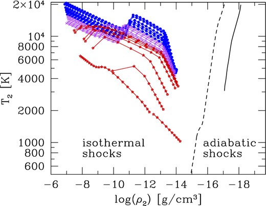
Post-shock density and temperature of the gas, immediately behind the shock front, as determined by the Rankine–Hugoniot conditions. Each track shows the evolution of the post-shock conditions as the shock propagates across the CSE from r = 1R to r = 5R, and refers to the quiescent condition (pre-flash luminosity maximum) just prior to the occurrence of each thermal pulse experienced by the Mi = 2.6 M⊙ and Zi = 0.017 model. Symbols are colour-coded as a function of the photospheric C/O ratio: blue for M stars, purple for S stars and red for C stars. The diagonal solid and dashed lines roughly mark the separation between shocks of predominantly isothermal and predominantly adiabatic character, following the detailed analysis of Woitke (1997, see text for more details).
Gas elements that are shocked to the left of the critical cooling tracks can re-establish radiative equilibrium before the next shock arrives (dominant isothermal character). Those which are shocked to the right of the critical cooling track will be hit by the next shock before radiative equilibrium can be achieved (dominant adiabatic character).
We notice that the post-shock values of temperature T2 and density ρ2 predicted with our shock models typically lie in the region where τcool ≪ P. As a consequence, we expect that the periodic shocks that hit the gas in the high-density inner CSE (within a few R) present a dominant isothermal character.
In the shock formalism adopted in the present study, isothermality corresponds to assuming a low value for |$\gamma _{\rm ad}^{\rm eff}$|, close to unity, which is in excellent agreement with the findings we have derived from the analysis of the HCN concentrations just discussed above. It is important to emphasize that the isothermal character of the shocks that emerge in the inner zone of the CSEs, derived from the detailed physical modelling of Woitke (1997), nicely provides physical independent support for our calibration analysis, which is, instead, based on a purely chemistry-related ground.
4.2.2 The shock formation radius
The shock formation radius rs,0 is another critical parameter of our chemo-dynamic model, since it determines the boundary between the static region and the pulsation-shocked region in the extended atmosphere, across which the average pre-shock density profile is expected to decrease with two quite different scale heights, as described in Section 3.2.
Since the static scale height H0 is shorter than the dynamic scale height Hdyn by a factor |$(1-\gamma _{\rm shock}^2)$|, it is clear that the farther the location rs,0, the lower the densities in the pulsation-shocked region. The density, in turn, affects the integration of the non-equilibrium chemistry network, hence, the concentrations of the different species.
Studies of pulsation-shocked chemistry dealing with the CSE chemistry of individual AGB stars, which are based on the Cherchneff et al. (1992) formalism for the density, locate the shock formation radius at typical distances rs,0 = 1.0, 1.2 and 1.3R (Cherchneff et al. 1992; Willacy & Cherchneff 1998; Duari et al. 1999; Duari & Hatchell 2000; Cau 2002; Agúndez & Cernicharo 2006; Cherchneff 2006, 2011, 2012; Agúndez et al. 2012).
On the theoretical ground, early numerical models of pulsating atmospheres (Willson & Bowen 1986; Bowen 1988) show that the position of the material when it first encounters the shock wave rs,0, the maximum shock amplitude Δυ0 and the pulsation period P (in a given mode) are interrelated quantities. In general, the larger the maximum shock amplitude, and hence, the higher γshock, the deeper in the atmosphere the first shock is expected to develop. We see that in many cases with higher shock amplitudes, rs,0 may be located even below the photosphere.
We have investigated the effect of the shock formation radius on the non-equilibrium HCN abundances, testing three values, i.e. rs,0/R = 1.2, 1.1 and 1.0. For simplicity, we assume that the minimum value for rs,0 is the photospheric radius. The predicted concentrations of HCN/H2 are displayed in Fig. 14 for rs,0/R = 1.2 and 1.1, while the results for rs,0/R = 1.0 are presented in the bottom-right panel of Fig. 12. In all three cases, the results are derived from non-equilibrium chemistry computations over the distances 3 ≤ r/R ≤ 5, during the entire TP-AGB evolution of the reference Mi = 2.6 M⊙ and Zi = 0.017 star.
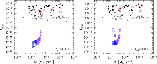
Comparison between observed CSE concentrations fHCN and the values obtained from shock-chemistry models for two choices of the shock formation radius rs,0 = 1.1R and rs,0 = 1.2R. In both computations |$\gamma _{\rm ad}^{\rm eff}=1.01$| is used.
It is evident that the models with rs,0/R = 1.2 and 1.1 fail to explain the observed data for both M and S stars, predicting HCN abundances that are far too low. Instead, the comparison is satisfactory for C stars. The main reason for the discrepancy that affects the M and S models should be ascribed to the gas densities that are too low across the pulsation-shocked region. On the other hand, a very nice agreement for all chemical classes, that is, at increasing photospheric C/O ratio from below to above unity, is achieved by the model with rs,0/R = 1.0. The same indication is obtained when considering other TP-AGB stellar tracks with different initial masses.
In summary, our tests indicate that the non-equilibrium shock chemistry in the inner CSEs can account for the measured HCN abundances, provided that the first shock emerges quite close to the star, from the photospheric layers. It is encouraging to realize that this stringent finding, derived from a chemistry-based calibration, is in line with other independent analyses carried out on both theoretical and observational grounds. Indeed, current detailed models of pulsating atmospheres for Mira variables indicate that pulsation-driven shocks form in the deep atmosphere, even below the photosphere, from where they propagate outward (Höfner et al. 1998, 2003; Nowotny et al. 2005, 2011). Observational support for an inner atmospheric origin of the shocks comes from the velocity and temperature structures derived from the vibration-rotation CO Δυ = 3 emission lines, which are consistent with the development of shock waves originating deeper than the line-forming layers (Hinkle, Scharlach & Hall 1984). Likewise, studies based on envelope tomography of long-period variables suggest that the double absorption lines in their optical spectra are caused by the propagation of a shock wave through the photosphere (Alvarez et al. 2001).
4.3 Non-equilibrium chemistry: major routes to HCN formation
We will discuss here the major chemistry channels involved in the formation of the HCN molecule across the shocked inner CSE. The chemo-dynamic integrations are carried out with the best-fitting parameters, rs,0/R = 1 and |$\gamma _{\rm ad}^{\rm eff}=1$|.
Fig. 15 (left-hand panel) neatly shows that the HCN abundances do depend on their photospheric C/O ratio. For any given C/O, after an initial decrease down to a minimum (much more pronounced for M stars) in the region very close to the star, the HCN concentration starts increasing from r/R ≈ 2 until it reaches a well-defined value that remains almost constant at larger distances. The level of the plateau is seen to increase systematically moving through the domains of M stars (C/O < 0.5), S stars (0.5 ≲ C/O ≲ 1.0) and C stars (C/O > 1.0).

Radial profiles of fHCN concentration across the r = 1–5R CSE, accounting for the non-equilibrium chemistry affected by the shocks. For each radius, chemistry predictions are shown after the completion of two consecutive pulsation cycles. The results of the chemo-dynamic integrations are connected to detailed TP-AGB evolutionary calculations. Each line corresponds to the stellar evolutionary stage just preceding a thermal pulse, experienced by our reference model with initial mass Mi = 2.6 M⊙ and metallicity Zi = 0.017. The assumed dynamic parameters are rs,0 = 1R and |$\gamma _{\rm ad}^{\rm eff}=1.01$|.
This finding is in contrast with the analysis of Cherchneff (2006), who predicted the presence of HCN in large quantities for any C/O ratio. That circumstance was ascribed to the very fast chemistry occurring in a very narrow region just after the shock front itself, as described by Willacy & Cherchneff (1998).
In any case, our calculations point at a different conclusion compared to the study of Cherchneff (2006). As an illustrative case, we will analyse the results obtained for the shock chemistry of an oxygen-rich CSE characterized by a photospheric C/O = 0.41 (Fig. 16). The stellar parameters refer to the quiescent stage just prior to the fourth thermal pulse experienced by a star with initial mass Mi = 2.6 M⊙ and metallicity Z = 0.017. In this respect, it is worth examining the evolution of the H2, CN and HCN concentrations, which results from both the very fast chemistry at the shock front and the chemistry during the subsequent post-shock relaxation phase.
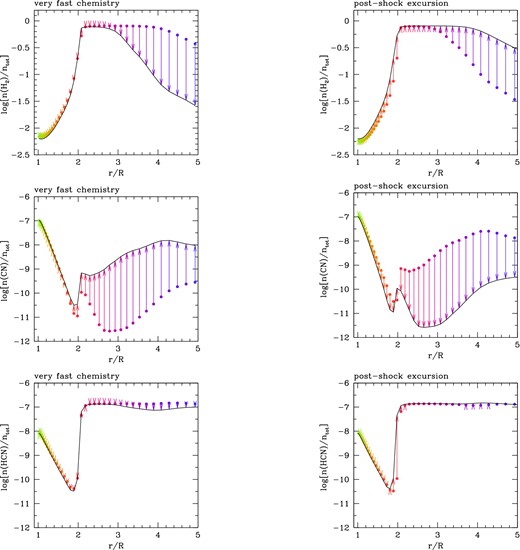
Results for the non-equilibrium chemistry for H2, CN and HCN, which occurs (a) in the very fast chemistry zone close to the shock front (left-hand panels) and (b) during the subsequent post-shock relaxation (right-hand panels). For each molecule, the arrows show the total variation in the molecule's fractional abundance, relative to the total number density, in the two regimes at any given distance across the CSE. In the left-hand panels, the dots mark the pre-shock abundances while the solid line connects the abundances reached just before the onset of the relaxation. These latter are taken as initial values of the post-shock expansion and are drawn with dots in the right-hand panels, while the solid line connects the abundances at the completion of one pulsation cycle. Note the steep increase of the H2 abundance for r/R ≲ 2 during the post-shock excursion phases, which is crucial for the formation of HCN (see equation 22). The stellar parameters correspond to the quiescent stage just prior to the fourth thermal pulse experienced by a star with initial mass Mi = 2.6 M⊙, metallicity Z = 0.017 and current photospheric C/O = 0.41.
Let us now examine the results of the chemistry during the post-shock excursion (right-hand panels of Fig. 16). Here the trends appear opposite compared to the very fast chemistry. In particular, we note that the concentration of H2 starts to increase steeply at inner radii, r/R < 1.5, quickly reaching a plateau that corresponds to the condition in which almost all hydrogen atoms are locked into H2.
The chemistry of H2 has a dramatic impact on the abundance of HCN. After an initial drop in the inner regions, the HCN concentration increases suddenly by a notable amount, just where H2 attains its maximum concentration, at r/R ≈ 2. Then, HCN levels off at n(HCN)/ntot ≈ 10−7, which is maintained across larger distances.
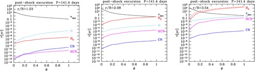
Relevant timescales during the post-shock excursion of the gas as a function of the phase at three different radial distances. The stellar parameters correspond to the quiescent stage just prior to the fourth thermal pulse experienced by a star with initial mass Mi = 2.6 M⊙, metallicity Z = 0.017 and current photospheric C/O = 0.41.
It is clear from equations (22) and (23) that the equilibrium abundances of HCN and CN are critically dependent, in opposite ways, on the ratio of molecular to atomic hydrogen, |${n(\rm {H}_2)}/{n(\rm {H})}$|. It is, therefore, important to analyse the behaviour of molecular hydrogen during the post-shock relaxation, at increasing distance from the star.
Fig. 18 (top panels) displays the evolution of the ratio |$f_{{\rm H}_2} \equiv n(\text{H}_2)/[0.5 n(\text{H}) + n(\text{H}_2)]$| as a function of the pulsation phase during the post-shock expansion of a fluid element that is hit by a shock at increasing distance from the star. Comparing the results obtained with the non-equilibrium chemistry network (left-hand panel) and with the assumption of ICE of all species (right-hand panel), we see that in both cases at a given distance (along each line), a rapid increase of |$f_{{\rm H}_2}$| takes place in the very initial phases, followed by a steady decrease during the following post-shock expansion. This trend is reversed at larger distances, where hydrogen atoms almost become trapped into H2 and |$f_{{\rm H}_2} \simeq 1$| during the entire post-shock relaxation, at any phase. In this respect, the major difference is that for the non-equilibrium chemistry case, |$f_{{\rm H}_2}$| reaches unity quite close to the star (r/R ≳ 2) when the gas density is still relatively high, but under the ICE condition, molecular hydrogen is efficiently formed farther from the star (r/R ≳ 3.5), so that |$f_{{\rm H}_2} \simeq 1$| in regions where the density has already dropped considerably.
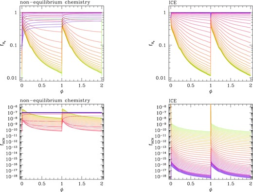
Evolution of the fractional concentrations of H2 and HCN as a function of the phase over two consecutive pulsation periods during the post-shock relaxation. Within the adopted Lagrangian framework, each line shows the abundance evolution experienced by a parcel of gas when it is hit by the outward propagating shock at a specific distance from the star. Each distance of the spatial grid is defined by a colour gradually changing along the sequence green–red–blue moving from r/R = 1 to r/R = 5. The results in the left-hand panels correspond to non-equilibrium chemistry calculations, while those in the right-hand panels are obtained under the assumption of ICE for all chemical species. Calculations refer to the same TP-AGB model as in Fig. 16.
The evolution of the HCN abundance reflects this difference in the evolution of H2 (bottom panels of Fig. 18). For the non-equilibrium chemistry, as soon as |$f_{{\rm H}_2} \simeq 1$| is attained, the concentration of HCN increases steeply, levelling out at fHCN ≈ 10−7, which is kept constant at larger radii, independently of the phase. Conversely, in the ICE case, the condition |$f_{{\rm H}_2}\simeq 1$| is reached only at longer distances, in low-density regions where the CN abundance is quite low. Hence, the concentration of HCN keeps on decreasing as the shock propagates outward.
Fig. 19 shows the radial abundance profiles of the species involved (H, O, H2, OH, H2O, CN and HCN) obtained by connecting the results soon after the completion of two pulsation periods (at phase ϕ = 2) at each mesh point of the spatial grid. Similar plots can be built at other phases. In general, one should be aware that radial abundance profiles obtained by connecting loci of equal phases may differ depending on the selected pulsation phase. This is evident, for instance, looking at Fig. 18. However, observations are compared with the predicted HCN abundances that are reached in the freeze-out region (3 ≲ r/R ≲ 5) where the phase dependence disappears.
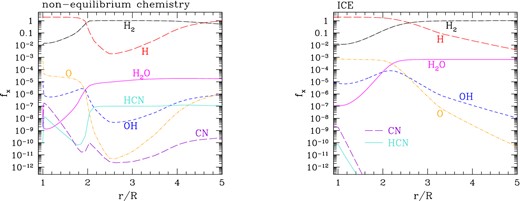
Radial profiles of the fractional concentrations of H, O, OH, H2, H2O, CN and HCN with distance from r/R = 1 to r/R = 5. They are obtained by connecting the abundances reached at each mesh point of the CSE (which defines a shocked fluid element in the Lagrangian scheme) soon after the completion of two pulsation periods (ϕ = 2) after the passage of the shock. Calculations refer to the same TP-AGB model as in Fig. 16. Left-hand panel: Results of the integration of the non-equilibrium chemistry network. Note the abrupt increase of fHCN up to ≃10−7, which takes place at r/R ≃ 2, just where |$f_{\rm {H}_2}$| rises to 1 and |$f_{\rm {H}_2O}$| exceeds fOH. Right-hand panel: Results obtained under the assumption of ICE for all chemical species. Note the severe drop of fHCN and fCN that starts close to the star.
It is evident that the predictions from the non-equilibrium chemistry (left-hand panel) are quite different from the ICE results. The passage of shocks favours the efficient formation of H2 in regions closer to the star, compared to the ICE case (right-hand panel). At r/R ≃ 2, 99 per cent of H atoms are locked into molecular hydrogen according to the non-equilibrium chemistry integrations, while for ICE, the fraction of molecular hydrogen is much less, |$f_{{\rm H}_2} \simeq 30 per cent$| and increases to |$f_{{\rm H}_2} \simeq 100 per cent $| at larger distances, from r/R ≳ 3.5.
Completely different results are obtained under the ICE assumption (right-hand plot of Fig. 19): the fractional abundances of HCN and CN exhibit a steadily decreasing trend across the CSE, quickly sinking to extremely low values.
In conclusion, our analysis shows that a proper treatment of the H–H2 chemistry in the inner shocked CSE during the post-shock relaxation stages is critical for the abundances of HCN and CN. In particular, the ICE assumption is inadequate and leads to a systematic underestimation of the HCN concentration, at least for the chemical mixtures characterized by C/O <1.
4.4 Additional effects: HCN abundance evolution through the thermal-pulse cycle
The results discussed in the previous sections apply to the quiescent TP-AGB evolution, so that each envelope integration corresponds to the stellar parameters at the stage just prior to the development of a thermal pulse.
However, stellar models show that the TP-AGB phase cannot be represented only by quiescent stages, since the quasi-periodic occurrence of thermal instabilities of the He-burning shell cause significant variations of the stellar structure, modulating the evolution of the luminosity according to a typical profile that is exemplified in Fig. 20. Denoting with τip the inter-pulse period between two consecutive He-shell flashes, we define the phase over a thermal-pulse cycle as ϕtpc = t/τip, where t is the time counted from the occurrence of a flash (ϕtpc = 0) up to the stage just prior to the next one (ϕtpc = 1).
![Evolution of stellar luminosity [L⊙], effective temperature [K], photospheric mass density [g cm−3], mass-loss rate [M⊙ yr−1], total mass [M⊙], pulsation period [d] in the fundamental mode, and fHCN concentration derived from shock-chemistry integrations at the radial distance r/R = 3, during the fifth, 10th and 16th pulse cycles of a TP-AGB model with initial mass Mi = 3.0 M⊙ and metallicity Zi = 0.017. The results are shown as a function of the phase, starting from ϕtpc = 0, at the onset of the He-shell flash, up to ϕtpc = 1, at the end of the inter-pulse period, just prior to the development of the next thermal pulse. The rapid post-flash maximum stages take place for ϕtpc ≲ 0.1. Black circles and starred symbols mark the selected phases (0.1 ≤ ϕtpc ≤ 1.0) at which chemo-dynamic integrations of the inner CSE are carried out (see also Fig. 21). Note the different morphologies and ranges covered by the HCN abundance tracks (bottom panels), depending on the photospheric C/O ratio and the other stellar parameters.](https://oup.silverchair-cdn.com/oup/backfile/Content_public/Journal/mnras/456/1/10.1093/mnras/stv2547/2/m_stv2547fig20.jpeg?Expires=1749877888&Signature=0CNKdJjzM9FARGY88C09uy-R6bFhcilnquXmwQxCLxfGoHlU2dM~ER5KfjmavocF7AkMzlLpOvdRAi23gE9iy5t0foK0dEJgu9bDiPSWnB~YHOXVji0Vk60-vfSDktWApXtZHXH9VGLqvgdO5IxZxItYpFRUonunw0UHj1h4yhBBGkqAG7hKXQwtSK14VR8NiseXNREGGW9oFn7RyO1656ywVOFbmD0pYhptnQ8v0Cc6SjYFdDSNcv4wIccYpepVRaMeJG4ArjrM5CYtt~twBBxadi-81EgMQB3sNeL5-KfcMt3hgkXqKmxUn~amJBYFAtA3KfxMnjHEzXrpY0DYpQ__&Key-Pair-Id=APKAIE5G5CRDK6RD3PGA)
Evolution of stellar luminosity [L⊙], effective temperature [K], photospheric mass density [g cm−3], mass-loss rate [M⊙ yr−1], total mass [M⊙], pulsation period [d] in the fundamental mode, and fHCN concentration derived from shock-chemistry integrations at the radial distance r/R = 3, during the fifth, 10th and 16th pulse cycles of a TP-AGB model with initial mass Mi = 3.0 M⊙ and metallicity Zi = 0.017. The results are shown as a function of the phase, starting from ϕtpc = 0, at the onset of the He-shell flash, up to ϕtpc = 1, at the end of the inter-pulse period, just prior to the development of the next thermal pulse. The rapid post-flash maximum stages take place for ϕtpc ≲ 0.1. Black circles and starred symbols mark the selected phases (0.1 ≤ ϕtpc ≤ 1.0) at which chemo-dynamic integrations of the inner CSE are carried out (see also Fig. 21). Note the different morphologies and ranges covered by the HCN abundance tracks (bottom panels), depending on the photospheric C/O ratio and the other stellar parameters.
Looking at Fig. 20, we see that during the first stages of a thermal-pulse cycle, a TP-AGB star is expected to have luminosities that may be much fainter than the quiescent values at ϕtpc ≈ 1, due to the low nuclear activity, or even extinction, of the H-burning shell.
The duration of these dimmer stages becomes longer for decreasing stellar mass, and it can cover up to 30–40 per cent of the inter-pulse periods in TP-AGB stars with masses ≲ 2 M⊙(Boothroyd & Sackmann 1988; Wagenhuber & Groenewegen 1998). It follows that the statistical significance of the post-flash sub-luminous phase, known by the global term of the low-luminosity dip, cannot be neglected in terms of detection probability.
During the low-luminosity dip, the star is characterized by significant variations of all other physical quantities, namely higher effective temperatures Teff, shorter pulsation periods P0 and lower mass-loss rates |$\dot{M}$|. Fig. 20 shows the evolution of these quantities over the fifth, 10th and 16th thermal-pulse cycles experienced by a TP-AGB model with initial mass Mi = 3.0 M⊙ and metallicity Zi = 0.017.
Since L, Teff, M, P and |$\dot{M}$| are the key input parameters of the present chemo-dynamic model for the inner CSE, it is worth exploring the effect of the pulse-driven variations of the stellar structure on the pulsation-shocked chemistry of HCN. Hence, we applied the chemo-dynamic integrations for 10 values of the pulse-cycle phase, from ϕptc = 0.1 to ϕptc = 1.0.
Fig. 20 provides an example of how the stellar parameters evolve, together with the resulting HCN non-equilibrium abundances in the inner CSE, during three complete thermal-pulse cycles. The pulses were selected to form a sequence of increasing photospheric C/O ratio (0.43, 0.74 and 1.31), to represent the three chemical classes of M, S and C stars. We note that, indeed, the HCN concentrations are affected by the occurrence of thermal pulses. When C/O = 0.43, the HCN abundance is seen to increase during the initial pulse-cycle phases up to the maximum value reached at ϕtpc ≃ 0.1, and then it decreases at later phases up to the completion of the inter-pulse period. For the models with C/O = 0.74 and 1.31, the trends are reversed, as the HCN concentrations reach a minimum at ϕtpc ≃ 0.3 and then increase for the remaining part of the thermal-pulse cycle.
Other test calculations were carried out for a few selected thermal pulses of TP-AGB models that are expected to undergo the transitions of the chemical types M → S → C, following the increase of the photospheric C/O ratio caused by the third dredge-up events. The results are shown in Fig. 21 for six choices of the initial stellar mass, Mi = 1.6, 1.8, 2.2, 2.6, 3.0 and 4.0 M⊙.
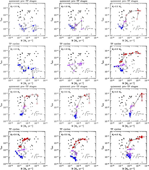
Predicted abundances fHCN in the inner CSE (3 ≤ r/R ≤ 5) as a function of the mass-loss rate during the entire TP-AGB evolution of six models with initial mass Mi = 1.6 M⊙, 1.8 M⊙, 2.2 M⊙, 2.6 M⊙, 3.0 M⊙ and 4.0 M⊙, and metallicity Zi = 0.017. The numbers quoted in the plots refer to the selected thermal pulses. From top to bottom, the panels are organized as follows. Odd rows: For each value of Mi, the sequence of empty symbols corresponds to the pre-flash luminosity maximum stage (pulse-cycle phase ϕ = 1.0 in Fig. 20) over the whole TP-AGB evolution. Colour-coding and symbols depend on the photospheric C/O ratio and are the same as in Fig. 11. Filled symbols and numbers are used to mark selected thermal pulses. Even rows: Evolution of the HCN abundance along the selected thermal-pulse cycles, identified by the corresponding number. Filled symbols are drawn for 10 discrete phases, 0 ≤ ϕtpc ≤ 1, in steps of Δϕtpc = 0.1
The variations of the HCN concentrations over a thermal-pulse cycle contribute to the observed scatter of the data belonging to the three chemical classes M, S and C. It is also worth noticing that the evolution of the HCN abundances covers a relatively wide interval of mass-loss rates, while it remains well inside the concentration boundaries of the three chemical types drawn by the measured data.
For instance, over the 19th pulse cycle experienced by the Mi = 2.2 M⊙ TP-AGB model, the corresponding HCN track performs a wide excursion in terms of the mass-loss rate – ranging from |$\dot{M}\approx 10^{-7}\,{\rm M}_{{{\odot }}}\,{\rm yr}^{-1}$| to |$\dot{M}\approx 2 \times 10^{-5}\,{\rm M}_{{{\odot }}}\,{\rm yr}^{-1}$| – and the predicted abundances are in excellent agreement with the observed location of the C-star data.
5 TOWARDS A CONSISTENT CHEMO-DYNAMIC PICTURE OF THE INNER CSE
The present work has, for the first time, coupled the evolution of a star during the TP-AGB phase to the non-equilibrium molecular chemistry that is expected to be active in the inner pulsation-shocked zone of its CSE.
To model the chemo-dynamic properties of the shocked gas in the region that extends from the stellar photosphere to a few stellar radii, we adopted the main scheme developed by Willacy & Cherchneff (1998), but introducing a few important changes. The purpose is to provide an approach that is able to handle more general cases (i.e. with all stellar parameters that vary along a TP-AGB track) and to ensure a higher level of self-consistency. In this respect, we performed the following steps:
First, we relax the common assumption of a constant shock parameter γshock, which was assigned a value of 0.89 in several past studies. Since γshock actually fixes the extended scale height for the pre-shock density profile in the shocked region, its value is now determined with the aid of a suitable continuity condition for the density at the dust condensation radius. In practice, the boundary condition involves finding the zero of a function in which all stellar parameters are involved. In this way, γshock is naturally predicted to vary during the TP-AGB evolution.
Secondly, once γshock is known, the maximum shock amplitude Δυ0 follows straightforwardly from the definition Δυ0 = γshock × υe. In past studies, Δυ0 was often chosen independently from γshock. We find that Δυ0 anti-correlates with the pulsation period, in close agreement with detailed models of pulsation-shocked atmospheres for AGB stars. Moreover, our predictions for the pre-shock radial profiles of the gas density and temperature compare nicely with the time-averaged spatial gradients derived by state-of-the-art dynamic atmosphere models for pulsating mass-losing AGB stars.
Thirdly, we take the remaining two shock parameters, rs, 0 and |$\gamma _{\rm ad}^{\rm eff}$|, as free quantities to be calibrated based on the HCN abundances measured in the CSEs of a populous sample of AGB stars of types M, S and C. Following the several tests made with different choices of the shock parameters, we eventually obtain a chemistry-based calibration of our dynamic model. The calibrated parameters are used to compute a large number of chemo-dynamic integrations of the inner CSEs, suitably tailored to an extended grid of TP-AGB evolutionary models. These provide the initial conditions to the CSE models in terms of key stellar properties: M, L, Teff, P, |$\dot{M}$|, ρphot and surface chemical composition, including the C/O ratio and the equilibrium molecular chemistry at the photosphere. In this way, a large variety of stellar conditions can be investigated.
The calibration procedure is successful and yields a nice agreement with the observed HCN abundances. Fig. 22 presents a comprehensive plot that includes many predicted values of the HCN concentrations in the inner CSEs, which correspond to models with different stellar masses and evolutionary stages during the TP-AGB. Our models recover the observed variation of the data as a function of the chemical type.
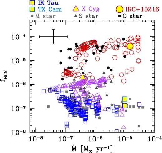
Comparison between observed HCN/H2 and predictions from our best-fit shock chemistry models applied to several TP-AGB tracks with initial masses in the range 1 M⊙ ≲ Mi ≲ 5 M⊙. All dynamic calculations for the inner CSE (with radial extension 1 ≤ r/R ≤ 5) are carried out with rs,0 = 1R and |$\gamma _{\rm ad}^{\rm eff}=1.01$|. We warn that the density of the theoretical points on the diagram is not indicative of detection probability, since we simply plot models from different tracks without simulating any synthetic sample of TP-AGB stars. Predicted abundances refer to the distance range 3 ≤ r/R ≤ 5 where the HCN chemistry is frozen out.
From the chemo-dynamic calibration, we derive important implications, which are summarized below.
5.1 Physical properties of the inner shocks
To have the suitably high densities needed to account for the observed HCN data, the shock formation radius should be located in the innermost zones of the CSE. The best results are obtained assuming rs,0 = R, which suggests that the shock waves caused by pulsation should emerge very close to the stellar photosphere. This finding is supported by independent observational and theoretical studies.
In the inner and denser zones of the CSEs, the shocks should exhibit a dominant isothermal character, which means that during the post-shock relaxation phase, the gas temperature cools primarily by emission of radiation. In our formalism, this condition corresponds to assuming low values for the effective adiabatic index, specifically |$\gamma _{\rm ad}^{\rm eff} \simeq 1$|. This indication is also in line with other independent findings obtained on empirical and theoretical grounds (e.g. see Fig. 13).
5.2 Chemistry routes to the formation of HCN and CN molecules
The ICE assumption is clearly violated in the shocked regions and is definitely inadequate to explain the measured HCN concentrations. In particular, for M and S stars, the ICE predictions underestimate the abundances by several orders of magnitude. In this respect, we confirm, for a larger base of stellar parameters, the indications from past chemical studies.
Our analysis suggests that the HCN abundance is critically linked to the H2–H chemistry during the post-shock relaxation phases, rather than to the very fast chemistry in the thin cooling layer as suggested by Cherchneff (2006).
5.3 Dependence of HCN concentrations on main stellar parameters
The calibrated models successfully account for the observed range of HCN abundances and measured mass-loss rates, extending up to both the minimum and maximum HCN values. The agreement supports the soundness of the underlying TP-AGB models in terms of C/O enrichment, evolution of effective temperature, pulsation period, stellar mass and radius, as well as to the appropriateness of the temperature, density and gas velocity profiles across the pulsation-shocked region.
We account for the variation of the HCN abundances as a function of the chemical type, neatly indicated by the observations of Schöier et al. (2013), with the mean values that increase along the sequence M-S-C. In this respect, we do not confirm the almost independence of HCN from the photospheric C/O ratio suggested by Cherchneff (2006). Interestingly, the models with 0.5 ≲ C/O ≲ 1.0 are found to cover a broader range of HCN concentrations, a feature that the measured data for S stars also show.
We investigate the effects on the non-equilibrium chemistry due to the variations of the stellar structure driven by thermal pulses. We find that the HCN concentrations may change significantly over a thermal-pulse cycle, contributing to the observed dispersion of the measured HCN data as a function of the mass-loss rates.
5.4 Caveats and planned improvements
We are aware of various limitations of our model, and are currently working on several improvements that will be addressed in follow-up works. These involve the assumption that fluid elements move on closed trajectories, the chemical effects of dust formation and, in general, the chemical network we are employing in this work. Here we briefly discuss these limitations, and why we believe that they can be safely neglected in the framework of this paper.
The chemical network used in this paper was originally developed by Cherchneff (2012) to model the C star IRC+10216. While it includes many reactions for O-bearing species, it is, however, possible that the network omits some reactions that are important for the chemistry of O-rich (M) stars. We are currently checking this aspect, and a revised/expanded network will be presented in a future paper. Here, it suffices to explore qualitatively the potential consequences upon the results of the present study.
We start from the basic consideration that HCN is a C-bearing species. Observations show that HCN abundances increase, on average, moving along the spectral sequence M-S-C (see Fig. 10), which indicates that the formation of HCN is strongly related to the amount of C that is not locked into CO molecules. In C stars, its abundance can reach values of the order of fHCN ∼ 10−5–10−4, whereas in M stars, HCN can only involve a residual (tiny) amount of C, and its concentration is typically much lower, fHCN ∼ 10−7.
Therefore, our naive expectation is that the addition of chemical species and reactions involving O-bearing species (e.g. a channel for the formation of water through ionic reactions) to the chemical network we used would not affect our results for C stars at all. Instead, in M (and, to a lesser extent, S) stars, such an addition might have an indirect effect: if a larger fraction of O atoms ends up in O-bearing species (e.g. water), the abundance of CO should decrease a bit compared to the value we calculated in our models. In turn, this should increase the amount of C that is available for other C-bearing species, such as HCN. Were this the case, reproducing the observed distribution of HCN abundances would require a change of the dynamical parameters, |$\gamma _{\rm ad}^{\rm eff}$|, γshock and rs,0. However, we expect such changes to be relatively small, otherwise we would lose the nice consistency of the dynamical picture obtained in this work, in particular with respect to the inner formation and the isothermal character of the shocks.
The model described in this paper does not account for the effects of dust formation on the chemical budget: in fact, the metals that condense into dust grains are no longer available for gas-phase chemistry (thus, at r > Rcond, we expect a significant depletion of Si and O in oxygen-rich stars, and of C in carbon-rich stars); furthermore, the very presence of dust might catalyse some reactions (e.g., H2 formation, Grassi et al. 2014, and references therein).
However, the HCN chemistry should be essentially unaffected by these inconsistencies. The reason is that in the majority of the cases we consider (i.e. for most of the TP-AGB evolution), dust formation takes place outside the region where the HCN abundance is changing. In fact, we generally have Rcond ≳ 2R for C stars, and Rcond ∼ 3–4R for M and S stars (see, e.g., Fig. 8), whereas the HCN abundance freezes out at ≲1.5R in C stars, and at ≲2.5R in M and S stars (see, e.g. Fig. 15). Thus, we believe that dust formation will not impact on the final abundances of HCN.
A further concern is that the newly condensed dust is likely to accelerate the stellar wind, thus taking the Lagrangian trajectories of fluid elements further away from our idealized assumption of strict periodicity with zero mass loss. However, first we note that for distances r ≲ 4 − 5R, the acceleration remains quite moderate, as can be seen in Fig. 8: for example, at r = 4R, the typical wind velocities are ≲4 km s−1, corresponding to a relative displacement Δr/r ≲ 0.03(P/1 yr)(r/1014 cm)−1. More importantly, for r > Rcond, fluid motions take place in the freeze-out region, so that inaccuracies in the description of the Lagrangian trajectories are not expected to produce significant effects on the HCN abundances.
For future developments of this work, we wish to revise the chemistry network to extend the analysis to other molecular species (e.g. H2O, NH3, SiO and SiS), and to explore the non-equilibrium chemistry of AGB CSEs at different metallicities. We aim at implementing dust growth in the shocked chemistry of CSEs, using the schemes already tested in recent studies (Nanni et al. 2013, 2014). We also plan to improve the prescriptions for the dynamics of the inner winds of TP-AGB stars, taking advantage of the results from state-of-the-art atmosphere models in which shocks, dust condensation and frequency-dependent radiative transfer are simultaneously included (Bladh et al. 2015; Eriksson et al. 2014).
This research is supported by the ERC Consolidator Grant funding scheme (project STARKEY, G.A. 615604). We also acknowledge support from the University of Padova (Progetto di Ateneo 2012, ID CPDA125588/12).
REFERENCES
