Cluster gas fraction as a test of gravity

Li, Baojiu; He, Jian-hua; Gao, Liang

doi:10.1093/mnras/stv2650

Abstract

We propose a new cosmological test of gravity, by using the observed mass fraction of X-ray-emitting gas in massive galaxy clusters. The cluster gas fraction, believed to be a fair sample of the average baryon fraction in the Universe, is a well-understood observable, which has previously mainly been used to constrain background cosmology. In some modified gravity models, such as f(R) gravity, gas temperature in a massive cluster is determined by the effective mass (the mass that would have produced the same gravitational effect assuming standard gravity as the cluster actually does in f(R) gravity) of that cluster, which can be larger than its true mass. On the other hand, X-ray luminosity is determined by the true gas density, which in both modified gravity and Λ-cold-dark-matter models depends mainly on Ω_b/Ω_m and hence the true total cluster mass. As a result, the standard practice of combining gas temperatures and X-ray surface brightnesses of clusters to infer their gas fractions can, in modified gravity models, lead to a larger – in f(R) gravity this can be 1/3 larger – value of Ω_b/Ω_m than that inferred from other observations such as the cosmic microwave background. Our quick calculation shows that the Hu–Sawicki n = 1 f(R) model with |$|\bar{f}_{R0}|=5\times 10^{-5}$| is in tension with the gas fraction data of the 42 clusters analysed by Allen et al. We also discuss the implications for other modified gravity models.

methods: analytical, methods: statistical, galaxies: haloes, cosmological parameters, dark matter, large-scale structure of Universe

1 INTRODUCTION

In recent years, attempts to understand the origin of the accelerated cosmic expansion (Riess et al. 1998; Perlmutter et al. 1999) have led to a large number of theoretical models (Copeland, Sami & Tsujikawa 2006). Apart from the current standard model, which assumes that the acceleration is caused by a cosmological constant Λ (hence the name Λ cold dark matter, or ΛCDM), these model can be roughly put in two categories: dark energy – which replaces Λ by some dynamical field, and modified gravity – which assumes that there is no exotic matter species beyond the standard CDM model but gravity is not described by general relativity (GR) on cosmological scales (see e.g. Clifton et al. 2012; Joyce et al. 2015, for some recent reviews). Some of the models in the latter class, such as the chameleon theory (Khoury & Weltman 2004), of which the well-known f(R) gravity (Carroll et al. 2005) is an example, have been active research topics in recent years.

Ultimately, any new cosmological model or theory of gravity should be put to rigorous tests against observational data. For this reason, a number of tests have been proposed or applied in the past to examine the viability of the models (see e.g. Lombriser 2014; De Martino, De Laurentis & Capozzilello 2015, for some recent reviews in f(R) gravity). The present paper shall follow the same line to propose a test using observations of galaxy clusters.

Galaxy clusters are the largest gravitationally bound and virialized objects in our Universe. The most massive clusters observed today typically have masses in the range of ∼10¹⁴–10¹⁵ h⁻¹ M_⊙, of which the dominant component is dark matter. These are homes to galaxies, stars and eventually lives, which together hold the vast majority of the information that can be extracted from cosmological and astrophysical observations. In dark energy or modified gravity theories, the different cosmic expansion histories and gravitational laws between particles can have sizeable effects on how the clusters form and evolve. Schmidt, Vikhlinin & Hu (2009) and Cataneo et al. (2015), based on this observation, have placed constraints on f(R) gravity using cluster abundance data. In theories such as f(R) gravity, massive and massless particles feel different strengths of gravity, thus allowing these theories to be constrained by comparing the so-called dynamical and lensing masses of clusters (Schmidt 2010; Zhao, Li & Koyama 2011). Combining with lensing observations, Terukina et al. (2014) and Wilcox et al. (2015) obtained even stronger constraints on f(R) gravity.

Given the abundant information associated with these rich objects, one expects that they will provide a wealth of other potential tests of new cosmological models. The arrival of the era of precision cosmology lends this perspective both more interest and more support. In this paper, we propose to utilize the observationally inferred mass fraction of hot X-ray-emitting gas in galaxy clusters as a new test of gravity.

The gas fraction in clusters, f_gas, is a well established and understood observable in the standard cosmological model, which can be used to place strong constraints on background cosmology (see e.g. Allen et al. 2004, 2008, and following-up works, for some examples). The basic assumptions (or approximations) are (i) clusters are in hydrostatic equilibrium between thermal pressure and gravity and (ii) as the largest objects in the Universe, the cluster baryon fraction, dominantly contributed by gas, is a faithful representation of the cosmological average baryon fraction Ω_b/Ω_m, in which Ω_b and Ω_m are, respectively, the fractional mass density of baryons and all matter (White et al. 1993; Eke, Navarro & Frenk 1998). Using (i), one can find, from the observed X-ray temperature and surface brightness profiles, the mass profiles of baryons and all matter inside a cluster, and consequently f_gas(r) – the profile of gas fraction. Combined with (ii), this can have a say about Ω_m provided that Ω_b is measured elsewhere (e.g. from big bang nucleosynthesis or the cosmic microwave background (CMB)).

In modified gravity theories, the hydrostatic equilibrium inside clusters is changed as a result of the different law of gravity. Hence, a cluster can have a higher dynamical mass, with the same baryonic mass inside, leading to a |$f_{\rm gas}^{\rm obs}$| that is lower than the true f_gas which is related to Ω_b/Ω_m. If a cosmologist wishes to infer Ω_b/Ω_m from |$f^{\rm obs}_{\rm gas}$| in a modified gravity universe, some correction has to be done to the end result, which can lead to inconsistencies with other observational determinations of Ω_b/Ω_m (for example the CMB), and hence a constraint on the gravity theory.¹ We shall demonstrate the potential constraints from this test using f(R) gravity as an example.

This paper is organized as following: in Section 2 we briefly describe the f(R) gravity theory and its equations which will be used in the discussion below. In Section 3, we give a more detailed account of the physics related to the gas fraction test described above. Then we present a numerical example in Section 4, which shows how current data of cluster gas fraction alone can give powerful constraints on gravity. We discuss the results and their implications in Section 5.

2 The f(R) gravity theory

This section is devoted to a quick overview of f(R) gravity. It will be kept brief and only include essential equations, given that there are already many papers in the literature covering this topic.

f(R) gravity (Carroll et al. 2005) is a simple generalization of GR, by replacing the Ricci scalar, R, in the Einstein–Hilbert action with an algebraic function f(R)

\begin{eqnarray} S = \int {\rm d}^4x\sqrt{-g}\left\lbrace \frac{1}{2}M_{\rm Pl}^2\left[R+f(R)\right]+\mathcal {L}_{\rm m}\right\rbrace , \end{eqnarray}

(1)

where M_Pl is the reduced Planck mass, |$M_{\rm Pl}^{-2}=8\pi \ G$| with G being Newton's constant, g is the determinant of the metric g_μν and |$\mathcal {L}_{\rm m}$| is the Lagrangian density for (normal plus dark) matter fields. The model is defined by specifying the functional form of f(R).

The action in equation (1) leads to a modified Einstein equation

\begin{eqnarray} G_{\mu \nu } + f_RR_{\mu \nu } -\left[\frac{1}{2}f-\Box f_R\right]g_{\mu \nu }-\nabla _\mu \nabla _\nu f_R = 8\pi GT^{\rm m}_{\mu \nu }, \end{eqnarray}

(2)

in which G_μν, R_μν are, respectively, the Einstein and Ricci tensors, f_R ≡ df/dR, ∇_μ the covariant derivative compatible to the metric g_μν, |$\Box \equiv \nabla ^\alpha \nabla _\alpha$| and |$T^{\rm m}_{\mu \nu }$| is the matter energy momentum tensor. Equation (2) can be considered as the standard Einstein equation of GR with an extra scalar field, f_R, whose dynamics is governed by

\begin{eqnarray} \Box f_R = \frac{1}{3}\left(R-f_RR+2f+8\pi G\rho _{\rm m}\right), \end{eqnarray}

(3)

where ρ_m is the mass density of baryons and dark matter. As we are interested in late times, photons and neutrinos will be neglected.

On scales well inside the Hubble radius, and for the models to be considered, it is safe to work with the quasi-static approximation (Bose, Hellwing & Li 2015), in which the scalar equation becomes

\begin{eqnarray} \nabla ^2f_R = -\frac{1}{3}a^2\left[R(f_R)-\bar{R} + 8\pi G\left(\rho _{\rm m}-\bar{\rho }_{\rm m}\right)\right], \end{eqnarray}

(4)

where ∇ denotes the three dimensional gradient, a is the scale factor and an overbar takes the background value of a quantity. Notice that R can be expressed as a function of f_R by inverting f_R(R).

Similarly, the modified Poisson equation in this limit reads as

\begin{eqnarray} \nabla ^2\Phi = \frac{16\pi G}{3}a^2\left(\rho _{\rm m}-\bar{\rho }_{\rm m}\right) + \frac{1}{6}a^2\left[R\left(f_R\right)-\bar{R}\right], \end{eqnarray}

(5)

where Φ is the Newtonian potential.

Equation (4) implies two limits of the behaviour of f(R) gravity:

When f_R is small, or more accurately, when |f_R| ≪ |Φ|, it recovers the well-known GR solution R = 8πGρ_m, and so equation (5) reduces to GR as well. This is the chameleon (Khoury & Weltman 2004) regime which any viable f(R) model must be in to pass the stringent Solar system and terrestrial tests of gravity.
When |$|f_R|\sim \mathcal {O}(|\Phi |)$|⁠, the second term on the right-hand side (rhs) of equation (5) is negligible compared with the first term, so that we have a gravity that is 1/3 stronger than in GR. This is usually known as the non-chameleon, or unscreened, regime.

It is evident that the unscreened regime mostly happens where Φ is shallow, or in extensive regions of low density. On large scales, matter density is close to the cosmological average, and so the total gravity in f(R) gravity is enhanced within scales comparable to the Compton wavelength of the scalar field f_R (which in most models of interest is in the range |$\mathcal {O}(1\sim 10)\,h^{-1}$|Mpc). This naturally leads to an enhanced large-scale structure formation, and features such as overabundant and more massive galaxy clusters – a topic which has been extensively studied previously. This will also be the topic that we focus on in this paper.

3 CLUSTER GAS FRACTION

Galaxy clusters are the largest bound objects in the Universe, whose masses are dominated by the dark matter component, with the baryonic masses dominated by X-ray-emitting intracluster gas, which is heated to temperatures of the order of keV during virialization. It is the mass fraction of this gas component that we will employ to test the theory of gravity here.

In this section, we shall first give a brief overview of how the baryon fraction can be estimated observationally, and how it can be used to constrain cosmological models and their parameters. Then, we will discuss how this process might be affected if the underlying theory of gravity is modified. For simplicity, we shall neglect other baryonic components than the intracluster gas in our analysis unless otherwise stated.

3.1 The standard ΛCDM model

In the standard cosmological scenario, halo density profiles can be universally described by the Navarro, Frenk & White (1997, NFW) fitting formula, which is often expressed as

\begin{eqnarray} \rho (r) = \frac{\rho _{\rm s}}{(r/r_{\rm s})\left(1+r/r_{\rm s}\right)^2}, \end{eqnarray}

(6)

in which ρ(r) is the halo mass density as a function of the distance, r, from the halo's centre, ρ_s is a characteristic density and r_s is the scale radius. We shall assume that the halo is spherically symmetric and well relaxed throughout the analysis, unless otherwise stated.

The mass of the halo can be obtained by integrating the NFW profile from r = 0 to r = R_Δ, in which R_Δ is the edge of the halo and is defined as the radius within which the average mass density is Δ × ρ_crit(z), with ρ_crit(z) ≡ 3H(z)²/8πG the critical density at the redshift z when the halo is identified. This leads to

\begin{eqnarray} M_{\rm halo} = 4\pi \rho _{\rm s}r^3_{\rm s}\left[\ln \left(1+R_\Delta /r_{\rm s}\right)-\frac{R_\Delta /r_{\rm s}}{1+R_\Delta /r_{\rm s}}\right]. \end{eqnarray}

(7)

Observationally, the total and baryonic masses of a cluster can be obtained by measuring its X-ray surface brightness profile, and the temperature profile of its X-ray gas. For a dynamically relaxed system that consists of dark matter and baryonic gas, a hydrostatic equilibrium can be achieved, which satisfies the following equation

\begin{eqnarray} \frac{1}{\rho _{\rm gas}(r)}\frac{{\rm d}}{{\rm d}r}P_{\rm gas}(r) = -\frac{GM_{\rm tot}(<r)}{r^2}, \end{eqnarray}

(8)

in which M_tot(< r) is the total mass of dark matter and gas within radius r, and ρ_gas(r), P_gas(r) are, respectively, the density and pressure of the gas at r. For simplicity, we neglect non-thermal pressure in our discussion (the effects of non-thermal pressure, however, are taken into account in the error budget when modelling the relation between f_gas and Ω_b/Ω_m, cf. equation (19) below).

For an ideal thermal gas, its pressure and density are related to its temperature, T_gas, as

\begin{eqnarray} P_{\rm gas} = kn_{\rm gas}T_{\rm gas} = \frac{k}{\mu m_{\rm p}}\rho _{\rm gas}T_{\rm gas}, \end{eqnarray}

(9)

where k is the Boltzmann constant, and the mass and number densities of the gas particles are connected by ρ_gas = μm_pn_gas, where m_p is the proton mass and μ the mean molecular weight. Applying equations (8) and (9), we obtain

\begin{eqnarray} \frac{G{M_{\rm tot}(<r)}}{r} = -\frac{kT_{\rm gas}(r)}{\mu m_{\rm p}}\left[\frac{{\rm d}\ln \rho _{\rm gas}(r)}{{\rm d}\ln r}+\frac{{\rm d}\ln T_{\rm gas}(r)}{{\rm d}\ln r}\right], \end{eqnarray}

(10)

which, if evaluated at the halo edge (⁠|$r=R_\Delta$|⁠), gives

\begin{eqnarray} \frac{GM_{\rm halo}}{R_\Delta } = -\frac{kT_{\rm gas}(R_\Delta )}{\mu m_{\rm p}}\left[\frac{{\rm d}\ln \rho _{\rm gas}}{{\rm d}\ln r}+\frac{{\rm d}\ln T_{\rm gas}}{{\rm d}\ln r}\right]_{r=R_\Delta }, \end{eqnarray}

(11)

in which M_halo is the total mass of dark matter and baryons within |$R_\Delta$|⁠.

In the mean time, the X-ray emission of galaxy clusters is produced mainly by thermal bremsstrahlung radiation, leading to a X-ray surface brightness profile that also depends on the gas density and temperature profiles, ρ_gas(r) and T_gas(r). In terms of gas density, the gas mass can be expressed as

\begin{eqnarray} M_{\rm gas}(<r) = \int ^r_04\pi r^{\prime 2}{\rm d}r^{\prime }\rho _{\rm gas}(r^{\prime }) \propto \rho _{\rm gas}(0)r_0^3, \end{eqnarray}

(12)

where ρ_gas(0) is the gas density at the cluster centre, and we have assumed that ρ_gas(r) = ρ_gas(0)g(r/r₀) with g(x) some function describing the profile and r₀ a characteristic scale. In the isothermal β model, for example, we have

\begin{eqnarray} \rho _{\rm gas}(r) = \rho _{\rm gas}(0)\left[1+\left(\frac{r}{r_0}\right)^2\right]^{-3\beta /2}, \end{eqnarray}

(13)

where β is a dimensionless constant.

The bolometric luminosity is given by (e.g. Sasaki 1996)

\begin{eqnarray} L_{\rm X}(<r) \propto \int ^r_04\pi r^{\prime 2}{\rm d}r^{\prime }T^{1/2}_{\rm gas}(r^{\prime })\rho _{\rm gas}^2(r^{\prime }) \propto \rho _{\rm gas}^2(0)r_0^3, \end{eqnarray}

(14)

where we have neglected the proportionality coefficients which are irrelevant here.

Combining equations (12) and (14), we have

\begin{eqnarray} M_{\rm gas} \propto L_{\rm X}^{1/2}r_0^{3/2} \propto d_{\rm L}f^{1/2}_{\rm X}\Theta _0^{3/2}d_{\rm A}^{3/2} \propto (1+z)^2d^{5/2}_{\rm A}, \end{eqnarray}

(15)

where d_L and d_A are, respectively, the luminosity and angular diameter distances and are related by d_L = (1 + z)²d_A. Here, we have used |$L_{\rm X}=4\pi d_{\rm L}^2f_{\rm X}$| where f_X is the X-ray flux, and r₀ = d_AΘ₀, in which Θ₀ denotes the angle spanned by r₀ at redshift z. Note that f_X (or equivalently the surface brightness) and Θ₀ are the observed quantities in this description. In real observations, one has the surface brightness and temperature profiles, or equivalently L_X(< r) and T_gas(r), using which equations (10) and (14) can be solved simultaneously to find M_halo(< r) and M_gas(< r) (note that the innermost regions of clusters are often excluded due to complicated processes such as cooling flow. For example, the study of Allen et al. (2008) uses only the data within 0.7 ∼ 1.2R₂₅₀₀ to measure f_gas). These provide the necessary information to find

\begin{eqnarray} f_{\rm gas}(r) = \frac{M_{\rm gas}(<r)}{M_{\rm halo}(<r)}. \end{eqnarray}

(16)

Often in observations, people quote the value of f_gas at r = R₂₅₀₀ as the cluster gas fraction. We note in passing that here M_halo enters the picture only through its gravitational effect on gas particles, as this fact is important for the discussion of modified gravity below.

To see how this can be used to constrain background cosmology, we note that, once the rhs of equation (11) is known by observations, we also have a fixed numerical value of the left-hand side and hence have the relation

\begin{eqnarray} M_{\rm halo} \propto R_\Delta \propto d_{\rm A}. \end{eqnarray}

(17)

Equations (15) and (17) imply that the measured cluster gas fraction depends on redshift and angular diameter distance in the following specific way:

\begin{eqnarray} f_{\rm gas}(z) = \frac{M_{\rm gas}}{M_{\rm halo}} \propto (1+z)^2d_{\rm A}^{3/2}. \end{eqnarray}

(18)

As mentioned earlier, we expect the cluster gas fraction to be a reasonably fair sample of the mean cosmological baryon fraction and is therefore roughly independent of z for massive clusters at low z. This is a reasonable assumption which should hold regardless of the cosmological model/parameters. The measurement of the apparent gas fraction, as described above, involves the angular diameter distance d_A and is indeed dependent on both the cosmological model and its parameters. Therefore, with incorrect cosmological models or parameters, the constancy of the true gas fraction (hereafter |$f_{\rm gas}^{\ast }$|⁠) is not guaranteed to be reflected in the observed value |$f^{\rm obs}_{\rm gas}(z)$|⁠. This provides a powerful test (Allen et al. 2004) of background cosmology and can be used to constrain cosmological parameters.

Were galaxy clusters perfectly fair samples of the average matter components in the Universe, their baryon fraction would just be Ω_b/Ω_m. The true situation, however, is more complicated. To take the complexities into account, Allen et al. (2008), improving on the earlier work of Allen et al. (2004), propose the following model of the relation between cluster gas fractions and Ω_b/Ω_m,

\begin{eqnarray} f^\ast _{\rm gas} = \frac{K\gamma b(z)}{1+s(z)}\frac{\Omega _{\rm b}}{\Omega _{\rm m}}, \end{eqnarray}

(19)

in which:

K is a constant accounting for systematic effects such as the calibration of instrument and X-ray modelling – it is assumed to be K = 1.0 ± 0.1 in Allen et al. (2008).
γ models the non-thermal pressure support in galaxy clusters which can cause a bias in the estimate of |$f^\ast _{\rm gas}$| of about 9 per cent.
b(z) ≡ b₀(1 + α_bz) is the so-called depletion factor which is inspired by the observation that the baryon fraction at R₂₅₀₀ in non-radiative simulations (Eke et al. 1998) is actually smaller than Ω_b/Ω_m, with b₀ = 0.83 ± 0.04 and α_b small indicating a weak redshift evolution below z = 1.
s(z) ≡ s₀(1 + α_sz) accounts for the fact that a small fraction of baryons can be in the form of stars, with s₀ = 0.16 ± 0.048 and −0.2 < α_s < 0.2 describing its redshift evolution.

The model in equation (19) indeed has a weak redshift dependence. However, any additional dependence from the observed f_gas would imply that one is using the wrong background cosmology to extract data, cf. equation (18). This is, to be clear, in the framework of standard GR.

3.2 Modified gravity scenarios

In many modified gravity theories, including f(R) gravity, the way in which the trajectories of massive test bodies – e.g. galaxies, stars and gas particles – respond to the underlying matter distribution is different. This change of the dynamics of test bodies is sometimes described as the change of the dynamical mass of matter. Massless particles, such as photons, could behave differently: in some theories, such as the Galileon model (Nicolis, Rattazzi & Trincherini 2009; Deffayet, Esposito-Farese & Vikman 2009) and the K-mouflage model (Brax & Valageas 2014a,b), photons can also feel a different mass of matter, but in other models, for example f(R) gravity and the Dvali, Gabadadze & Porrati (2000, DGP) model, photon trajectories depend on the matter distribution in essentially the same way as in GR, since the conformal coupling does not affect geodesics of massless particles. For distinction, the mass felt by photons is usually called the lensing mass. The differences in the dynamical and lensing masses of galaxy clusters have been used to constrain f(R) gravity in, e.g. Terukina et al. (2014) and Wilcox et al. (2015)

As mentioned above, gas particles, like dark matter particles and galaxies, do feel the dynamical mass of a cluster. In f(R) gravity, the same cluster can have a dynamical mass 4/3 times its value in GR. This maximum enhance factor of 1/3, however, is not necessarily realized in all clusters, because of the chameleon screening (Khoury & Weltman 2004). The screening helps to reduce the difference between the dynamical and lensing masses, especially for more massive clusters. Consequently, constraints relying on the dynamical masses of clusters are in general weaker than those coming from astrophysical considerations. Nevertheless, they have cleaner physics than that of astrophysical observables – which can often depend on whether the considered astrophysical system lives inside a screened cluster – and are amongst the tightest constraints obtained using cosmological data (Terukina et al. 2014).

Evidently, without a reliable measurement of the lensing mass, it is difficult to tell whether one observes a cluster of true mass M in GR, or one with a smaller mass in f(R) gravity, since both have the same dynamical masses. This has motivated He et al. (2015) to propose the concept of effective haloes. Briefly speaking, the idea is to redefine the rhs of the modified Poisson equation in f(R) gravity, equation (5), so that it can be rewritten as

\begin{eqnarray} \nabla ^2\Phi = 4\pi Ga^2\delta \rho _{\rm m,eff}. \end{eqnarray}

(20)

In the above, Φ is the Newtonian potential that determines the dynamics of massive bodies and |$\delta \rho _{\rm m}\equiv \rho _{\rm m}-\bar{\rho }_{\rm m}$| is the density perturbation of (dark plus baryonic) matter. δρ_m,eff is the effective density field, with which the Poisson equation takes exactly the same form as in GR (cf. equation 20). In this way, the complicated new physics in f(R) gravity is absorbed into ρ_{m, eff}, and with that solved (e.g. in numerical simulations) one can in principle proceed assuming GR as the true theory of gravity. He & Li (2015), for example, show with hydrodynamical simulations that cluster gas temperatures depend only on the masses of the corresponding effective haloes, and that with certain rescaling depending on the effective halo mass the scaling relations – such as the L_X–M relation with L_X the X-ray luminosity – in f(R) gravity can be derived reliably using existing knowledge of GR.

In the left-hand panel of Fig. 1, we present the gas temperature profiles for standard haloes in GR and effective haloes in f(R) gravity, both in the mass bin 10¹³ ∼ 10^13.4 h⁻¹ M_⊙. Though there are differences in the inner regions – which could be due to different halo density profiles or screening – we notice that beyond ∼100 h⁻¹ kpc the two agree very well. He & Li (2015) find that the average gas temperatures in the two also show very good agreement, and indeed the temperature–mass relation is barely distinguishable in the two models, provided that effective haloes are used in f(R) gravity.

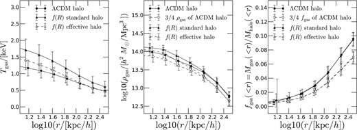
$Left-hand panel: the halo gas temperature profiles from the non-radiative hydrodynamical simulations of He & Li (2015) for the standard ΛCDM model (solid line with filled circles) and HS n = 1 f(R) gravity with $|\bar{f}_{R0}|=10^{-5}$ (solid line with filled triangles for standard haloes and dashed line with empty triangles for effective haloes. The error bars are standard deviations and the same line and symbol styles are used for the other two panels). Middle panel: the same as the left-hand panel, but for the gas density profiles. The dashed line with empty circles a rescaling of the ΛCDM curve by 3/4 to take into account the fact that for a ΛCDM halo and a f(R) effective halo of the same mass, their true masses differ by 1/3. Right-hand panel: The halo gas fraction profiles from the same simulations; the dashed line with empty circles is the ΛCDM result scaled by 3/4, which is almost identical to the result of f(R) effective haloes, cf. equation (21). The profiles shown here are stacked results of the haloes in the mass range 1013 ∼ 1013.4 h−1 M⊙, for illustration purpose. The mass range is chosen so that the haloes are unscreened for the f(R) model simulated, and we checked that results from other halo mass bins follow the same trends. For other f(R) parameters, such as the ones used in Section 4, unscreened haloes can be more massive and they are expected to show the same behaviour of fgas as seen here.$

Figure 1.

Left-hand panel: the halo gas temperature profiles from the non-radiative hydrodynamical simulations of He & Li (2015) for the standard ΛCDM model (solid line with filled circles) and HS n = 1 f(R) gravity with |$|\bar{f}_{R0}|=10^{-5}$| (solid line with filled triangles for standard haloes and dashed line with empty triangles for effective haloes. The error bars are standard deviations and the same line and symbol styles are used for the other two panels). Middle panel: the same as the left-hand panel, but for the gas density profiles. The dashed line with empty circles a rescaling of the ΛCDM curve by 3/4 to take into account the fact that for a ΛCDM halo and a f(R) effective halo of the same mass, their true masses differ by 1/3. Right-hand panel: The halo gas fraction profiles from the same simulations; the dashed line with empty circles is the ΛCDM result scaled by 3/4, which is almost identical to the result of f(R) effective haloes, cf. equation (21). The profiles shown here are stacked results of the haloes in the mass range 10¹³ ∼ 10^13.4 h⁻¹ M_⊙, for illustration purpose. The mass range is chosen so that the haloes are unscreened for the f(R) model simulated, and we checked that results from other halo mass bins follow the same trends. For other f(R) parameters, such as the ones used in Section 4, unscreened haloes can be more massive and they are expected to show the same behaviour of f_gas as seen here.

Open in new tab Download slide

The fact that the cluster gas temperatures depend on the mass of the effective haloes is as expected, since for relaxed systems the virial temperature depends on the Newtonian potential, which does not distinguish between standard (GR) and effective (f(R) gravity) density fields. For a polytropic gas with an equation of state |$P_{\rm gas}\propto \rho _{\rm gas}^\Gamma$| in which the constant Γ ≥ 1, the hydrostatic equation implies that (see e.g. Mo, van den Bosch & White 2011) the temperature can be analytically expressed as a function of the potential Φ.

Let us now consider two haloes, one identified in the standard dark matter field in a model with GR as the gravity theory, another from the effective density field in f(R) gravity. The profiles of the two haloes are the same so that equation (20) sees no difference in them. Since gravity only enters the picture through equation (10), we make the following two observations/predictions:

the gas temperature profiles are the same in these two haloes;
the two sides of the spherical hydrostatic equation, equation (10), are the same for the two haloes.

Since T_gas(r) and d ln T_gas(r)/d ln r in equation (10) are the same, we conclude that d ln ρ_gas(r)/d ln r is also the same in the haloes. This, however, does not necessarily mean that the haloes have identical gas density profiles, because we can rescale ρ_gas by a constant factor without changing d ln ρ_gas(r)/d ln r. To confirm this, in the middle panel of Fig. 1 we compare the gas density profile of f(R) effective haloes with that of ΛCDM haloes of the same mass, and find that the two show a constant shift by 1/4 beyond r ∼ 100 h⁻¹ kpc. Note that the simulated haloes in the plot do not have perfectly identical total – standard or effective – mass profiles, which is why in the middle panel of Fig. 1 the two dashed lines with open circles and open triangles do not agree on scales below ∼100 h⁻¹kpc. However, as mentioned above equation (22), in real observations, such innermost regions are not used in the determination of f_gas anyway.

As a result, to obtain the gas density profile, we need further, independent, information to fix its normalization – as opposed to its shape – which brings us back to the measurements of cluster X-ray surface brightness. Inspecting the equation for the cluster X-ray luminosity, equation (14), we notice that the luminosity density (i.e. the integrand) depends on (i) the physical gas density ρ_gas, and (ii) the gas temperature T_gas which, as we have seen above, depends on the total mass of the effective halo. Consequently, should the physical gas densities be the same for f(R) effective and ΛCDM haloes of the same mass, there would be no difference in their X-ray surface brightness profiles.

However, despite the standard (GR) and effective (f(R) gravity) haloes above having identical gas temperature and halo mass, their actual (physical, or lensing) masses are different, and it is important to remember that Ω_m characterises the amount of the actual mass in the Universe. If, as we have assumed so far, the gas fraction in clusters is a fair sample of the cosmological value, it would be the ratio of the gas mass and actual halo's mass that satisfies equation (19). Gas fractions inferred observationally, in the way described in the previous subsection, are in fact the ratio of the gas mass and that of the effective halo. If we denote the ratio of the effective and actual masses of a halo by η, then 1 ≤ η ≤ 4/3, depending on the actual mass and environment of the halo, its redshift, as well as the f(R) model parameters.² Here, as we are interested in the most massive clusters, with M_halo ∼ 10¹⁴–10¹⁵ h⁻¹ M_⊙, we can for simplicity neglect the impacts of the halo's environment, so that η mainly depends on z, i.e. η = η(z), for a given halo mass.

Consider the extreme case in which η = 4/3 as example. The apparent f_gas inferred from X-ray cluster observations would be

\begin{eqnarray} f^{\rm obs}_{\rm gas} = \frac{M_{\rm gas}}{M_{\rm halo, eff}} = \frac{3}{4}\frac{M_{\rm gas}}{M_{\rm halo,actual}} = \frac{3}{4}f^\ast _{\rm gas}. \end{eqnarray}

(21)

This is also confirmed by hydro simulations, as shown in the right-hand panel of Fig. 1. In that plot, we see that if haloes are defined using their actual masses in f(R) gravity, then they share the same f_gas as ΛCDM haloes of the same mass (the two solid lines). For effective f(R) haloes, on the other hand, their f_gas profiles are a constant downward shift by 1/4 from the results of ΛCDM haloes of the same masses (the two dashed lines), which is exactly what equation (21) predicts. Note that in our non-radiative simulations we have not included more complicated baryonic effects, such as AGN feedback, which is known to have a non-negligible impact on the cluster properties. Martizzi et al. (2014) notice that including this actually can improve the agreement of simulation prediction of f_gas with observations. Here, we assume that the AGN feedback in f(R) gravity is not drastically different from that in ΛCDM simulations, so that its inclusion does not change equation (21). It would be interesting to have more complete hydro simulations to study such effects in modified gravity in the future.

It is worthwhile to pause for a moment and try to understand the physics behind the behaviour of Fig. 1. It may seem surprising that, although the gas density profiles in ΛCDM and f(R) standard haloes are significantly different within r ∼ 100 h⁻¹ kpc, their gas fraction profiles are very close to each other. This suggests that the two also have different dark matter (or total) mass profiles to cancel the differences in ρ_gas(r). In other words, ρ_gas(r) follows ρ_DM(r), which is the physical dark matter mass density, in the same way in ΛCDM and f(R) standard haloes, even though they have different mass and even more different potential profiles. To understand this, we note that in equation (10) the G on the left-hand side and T_gas on the rhs are both modified in f(R) standard haloes. Indeed, if one assumes hydrostatic equilibrium and |$P_{\rm gas}\propto \rho ^\Gamma _{\rm gas}$|⁠, then the gas density profile can be written as (Komatsu & Seljak 2001)

\begin{eqnarray} \frac{\rho ^{\Gamma -1}_{\rm gas}(r)}{\rho ^{\Gamma -1}_{\rm gas}(0)} = 1- \frac{\Gamma -1}{\Gamma }\frac{G\mu m_{\rm p}M_{\rm halo}}{R_{\rm vir}kT_{\rm gas}(0)}\frac{c}{m(c)}\int ^{\frac{r}{r_{\rm s}}}_0\frac{m(x)}{x^2}{\rm d}x, \end{eqnarray}

(22)

in which |$m(r/r_{\rm s})\equiv M(<r)/4\pi \rho _{\rm s}r^3_{\rm s}$|⁠. Equation (22) is derived under the assumption of self-similarity of gas density profiles, but the key point therein, that the modified gravity effects on G and T_gas can be cancelled out, is not affected by this assumption. If this cancellation happens, then the gas density profile is determined by the total mass profile under the assumption of hydrostatic equilibrium, regardless of the theory of gravity.³

In clusters, gas is heated by accretion shocks during the assembly of the halo, a process which involves the conversions of energy from gravitational to kinetic (that of the cold accreted gas) and then to thermal (via shocks). Assuming a complete thermalization, the post-shock gas temperature is proportional to |$v_{\rm infall}^2$|⁠, with v_infall the infall speed of the accreted gas (e.g. Mo et al. 2011). Consequently, energy conservation implies that the final gas temperatures in the central regions will be affected in the same way as |$v_{\rm infall}^2$| of the cold gas and hence G in modified gravity. Of course, this is only an approximation, and the cancellation of the effects of modified gravity on G and T_gas depend on various factors including the screening and formation history of a cluster, which is not expected to be complete. However, Fig. 1 suggests that it works pretty well for the haloes we use here. We checked explicitly that it works slightly less well for more massive haloes, for which the agreement between the f_gas(r) in ΛCDM and f(R) standard haloes is slightly less perfect – this may be because those haloes became unscreened only very recently.

The argument above in theory also applies to effective haloes, for which G is the same as in GR, but the effects of modified gravity are incorporated in M_halo. However, in the effective halo case the normalization is different because of the different total gas fraction (see footnote 2) – although the shape is the same – hence the nearly constant rescaling of the dashed line with open triangles compared with the solid line with filled circles in Fig. 1.

Coming back to the discussion prior to the previous three paragraphs, our result suggests two possible tests of f(R) gravity:

If an observer actually lives in a universe shaped by f(R) gravity, then the true cluster gas fraction is given by |$f^{\ast }_{\rm gas}=\eta f^{\rm obs}_{\rm gas}$|⁠. Assuming that equation (19) still holds for |$f^\ast _{\rm gas}$|⁠, the observer will need to do the following transformation to get the true Ω_b/Ω_m:
\begin{eqnarray} f^{\rm obs}_{\rm gas} = \frac{1}{\eta }\frac{K\gamma b(z)}{1+s(z)}\left[\frac{\Omega _{\rm b}}{\Omega _{\rm m}}\right]_{\rm true} \Rightarrow \left[\frac{\Omega _{\rm b}}{\Omega _{\rm m}}\right]_{\rm true} = \eta \left[\frac{\Omega _{\rm b}}{\Omega _{\rm m}}\right]_{\rm obs}. \end{eqnarray}
(23)
As (Ω_b/Ω_m)_obs depends only on the actual observational data, the observer will obtain the same value as an observer in a standard GR universe would do. The resulting (Ω_b/Ω_m)_true might then be too large to be compatible with other constraints, such as the one from the CMB.
Alternatively, if one takes the Ω_b/Ω_m measured by other probes as the true value and starts from there, then equation (21) implies that the observed cluster gas fraction |$f^{\rm obs}_{\rm gas}$| will be smaller than what the ΛCDM model and simulations predict. Because of the time dependence of η(z) (see above), if the f(R) model parameters happen to take the values for η to evolve from 1 to 4/3 between z = 1 and the present for the clusters of interest, there may also be an apparent decrease of |$f^{\rm obs}_{\rm gas}(z)$| as z decreases, by a maximum of 25 per cent.

4 NUMERICAL EXAMPLES

In this section, we use a simplified example to illustrate the power of the cluster gas fraction test proposed above. For this, we will use the gas fraction data of the 42 clusters studied by Allen et al. (2008, table 3). As described above, these f_gas data are obtained by fitting the gas temperature and X-ray surface brightness profiles of these clusters simultaneously, assuming NFW profiles for the total mass in clusters. We have also found that, in the context of f(R) gravity, as long as we use effective haloes, the dynamics of gas particles can be calculated using standard gravity theory. Therefore, in this work we can directly take the data of Allen et al. (2008) as |$f^{\rm obs}_{\rm gas}$|, bearing in mind that the cluster mass inferred therein would be the effective mass and therefore |$f^{\rm obs}_{\rm gas}$| can be different from |$f^{\ast }_{\rm gas}$| for unscreened clusters, cf. equation (21).

To obtain an estimation of the mean and standard deviation of |$\left(\Omega _{\rm b}/\Omega _{\rm m}\right)_{\rm obs} = \frac{1+s(z)}{K\gamma b(z)}f^{\rm obs}_{\rm gas}$| from each cluster, random samples of size 10⁵ are drawn for each parameter or data: K, γ, b₀, α_b, s₀, α_s and |$f^{\rm obs}_{\rm gas}$|⁠. Of these, |$f^{\rm obs}_{\rm gas}$| is taken, for a given cluster, from table 3 of Allen et al. (2008), and is assumed to satisfy a Gaussian distribution with mean and standard deviation given by Allen et al. (2008). The other parameters and their distributions are shown in Table 1. We therefore obtain 10⁵ realizations of (Ω_b/Ω_m)_obs, from which its mean and standard deviation can be calculated. This procedure is repeated for all 42 clusters.

Table 1.

Open in new tab

The assumed ranges and distributions of the model parameters in equation (19). For more details the readers are referred to Section 3.1 or Allen et al. (2008).

Param	Physical effect described	Mean ± stddev	Prior
K	Overall calibration	1.000 ± 0.100	Gaussian
γ	Non-thermal pressure	1.050 ± 0.050	Uniform
b₀	Gas bias: normalization	0.825 ± 0.175	Uniform
α_b	Gas bias: evolution	0.000 ± 0.100	Uniform
s₀	Stellar fraction: normalization	0.160 ± 0.048	Gaussian
α_s	Stellar fraction: evolution	0.000 ± 0.200	Uniform

Param	Physical effect described	Mean ± stddev	Prior
K	Overall calibration	1.000 ± 0.100	Gaussian
γ	Non-thermal pressure	1.050 ± 0.050	Uniform
b₀	Gas bias: normalization	0.825 ± 0.175	Uniform
α_b	Gas bias: evolution	0.000 ± 0.100	Uniform
s₀	Stellar fraction: normalization	0.160 ± 0.048	Gaussian
α_s	Stellar fraction: evolution	0.000 ± 0.200	Uniform

Table 1.

Open in new tab

The assumed ranges and distributions of the model parameters in equation (19). For more details the readers are referred to Section 3.1 or Allen et al. (2008).

Param	Physical effect described	Mean ± stddev	Prior
K	Overall calibration	1.000 ± 0.100	Gaussian
γ	Non-thermal pressure	1.050 ± 0.050	Uniform
b₀	Gas bias: normalization	0.825 ± 0.175	Uniform
α_b	Gas bias: evolution	0.000 ± 0.100	Uniform
s₀	Stellar fraction: normalization	0.160 ± 0.048	Gaussian
α_s	Stellar fraction: evolution	0.000 ± 0.200	Uniform

Param	Physical effect described	Mean ± stddev	Prior
K	Overall calibration	1.000 ± 0.100	Gaussian
γ	Non-thermal pressure	1.050 ± 0.050	Uniform
b₀	Gas bias: normalization	0.825 ± 0.175	Uniform
α_b	Gas bias: evolution	0.000 ± 0.100	Uniform
s₀	Stellar fraction: normalization	0.160 ± 0.048	Gaussian
α_s	Stellar fraction: evolution	0.000 ± 0.200	Uniform

The estimation of the effects of modified gravity, i.e. the factor η(z), is more complicated, since it depends on the cluster mass, density profile, environment, redshift, as well as the f(R) parameters. Because the main purpose of this paper is to illustrate the basic idea, we shall leave a full analysis using real cluster data for future work, and instead adopt a simplified modelling. The cluster masses are assumed to be the same, with M_halo = 7.5 × 10¹⁴ h⁻¹ M_⊙, for all 42 clusters, as this is a typical value for massive X-ray clusters. The cluster's radius (R₂₀₀) is ∼1.5 h⁻¹ Mpc and its concentration parameter, c ≡ R₂₀₀/r_s is 3.3. The cluster is assumed to live on the cosmological background, so that the ratio of its effective and actual masses can be approximated as (see e.g. Li, Zhao & Koyama 2012)

\begin{eqnarray} \eta (z)=\frac{M_{\rm halo,eff}}{M_{\rm halo,actual}} = \min \left\lbrace 1+\frac{\bar{f}_R(z)}{2\Phi _{\rm N}},\frac{4}{3}\right\rbrace , \end{eqnarray}

(24)

where |$\bar{f}_R(z)$| is the background value of f_R at redshift z. However, as the observational data of f_gas are generally at R₂₅₀₀ rather than R₂₀₀, for a more realistic estimate of the screening effect we should replace M_halo in the above equation with M₂₅₀₀, and correspondingly evaluate Φ_N also at R₂₅₀₀:

\begin{eqnarray} {\Phi _{\rm N} = -\frac{GM_{2500}}{R_{2500}}\frac{\ln (1+c^{\prime })}{\ln (1+c^{\prime })-c^{\prime }/(1+c^{\prime })} \approx -8.1\times 10^{-5}}, \end{eqnarray}

(25)

where c′ ≡ R₂₅₀₀/r_s ≈ 0.88 with R₂₅₀₀ ≈ 0.4 h⁻¹Mpc.

We adopt the f(R) model by Hu & Sawicki (2007) with n = 1, for which

\begin{eqnarray} \bar{f}_R(z) = \left[\frac{\Omega _{\rm m}+4\Omega _\Lambda }{\Omega _{\rm m}(1+z)^3+4\Omega _\Lambda }\right]^2\bar{f}_{R0}. \end{eqnarray}

(26)

The values Ω_m = 0.316 and |$\Omega _\Lambda =0.684$| are taken from the latest results of Planck Collaboration XIII (2015). As a result, the physics of modified gravity is completely governed by |$\bar{f}_{R0}$|⁠, which is the present-day value of |$\bar{f}_R$|⁠. Once this is specified, we can obtain η(z), and therefore infer (Ω_b/Ω_m)_true given (Ω_b/Ω_m)_obs and z of a cluster.

In Fig. 2, we show the (Ω_b/Ω_m)_true result obtained from |$f^{\rm obs}_{\rm gas}$| for four different cases: standard ΛCDM (upper left), and f(R) gravity models with |$|\bar{f}_{R0}|=3\times 10^{-5}$| (upper right), 5 × 10⁻⁵ (lower left) and 10⁻⁴ (lower right). For comparison, we have also, in each panel, plotted the mean value (solid line) and 1σ confidence level (dotted) of Ω_b/Ω_m from Planck Collaboration XIII (2015).⁴ The results from the 42 clusters, with 1σ errors, are shown as symbols (here the variations across this sample of 42 clusters resemble the standard deviations displayed in the right-hand panel of Fig. 1).

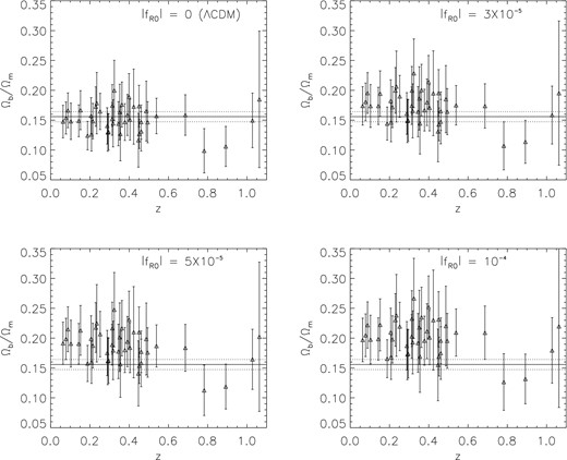
$The inferred Ωb/Ωm (triangles with 1σ error bars) using the $f^{\rm obs}_{\rm gas}$ for the 42 clusters from Allen et al. (2008), as a function of the cluster redshift. Four cases are shown, with different underlying models of gravity: GR (upper left), and Hu–Sawicki n = 1 f(R) model with $|\bar{f}_{R0}|=3\times 10^{-5}$ (upper right), 5 × 10−5 (lower left), 10−4 (lower right). The horizontal solid and dotted lines are, respectively, the mean and 1σ range of Ωb/Ωm from Planck CMB data. A good match between fgas and CMB for the GR case, and progressively worse matches for the f(R) models, can be seen by a quick inspection by eye. For simplicity, all haloes are assumed to have a mass of 7.5 × 1014 h−1 M⊙ and a concentration of 3.3 when determining the effect of the chameleon screening.$

Figure 2.

The inferred Ω_b/Ω_m (triangles with 1σ error bars) using the |$f^{\rm obs}_{\rm gas}$| for the 42 clusters from Allen et al. (2008), as a function of the cluster redshift. Four cases are shown, with different underlying models of gravity: GR (upper left), and Hu–Sawicki n = 1 f(R) model with |$|\bar{f}_{R0}|=3\times 10^{-5}$| (upper right), 5 × 10⁻⁵ (lower left), 10⁻⁴ (lower right). The horizontal solid and dotted lines are, respectively, the mean and 1σ range of Ω_b/Ω_m from Planck CMB data. A good match between f_gas and CMB for the GR case, and progressively worse matches for the f(R) models, can be seen by a quick inspection by eye. For simplicity, all haloes are assumed to have a mass of 7.5 × 10¹⁴ h⁻¹ M_⊙ and a concentration of 3.3 when determining the effect of the chameleon screening.

Open in new tab Download slide

A quick naked-eye inspection shows that the f_gas method and the CMB observation give compatible Ω_b/Ω_m if one assumes the ΛCDM paradigm (upper left). The f(R) model with |$|\bar{f}_{R0}|=10^{-4}$| (lower right), on the other hand, leads to a significantly higher value of Ω_b/Ω_m than what CMB says, and is therefore inconsistent. The other two cases are more interesting: for |$|\bar{f}_{R0}|=5\times 10^{-5}$| (lower left), η(z) increases to ∼1.3 at z = 0.05, while for |$|\bar{f}_{R0}|=3\times 10^{-5}$| (upper right) η(z) only increases to ∼1.18 at z = 0. In both cases, however, the inferred values of Ω_b/Ω_m are still substantially larger than the Planck result, especially for the low-z clusters. This shows that cluster gas fraction can be a potentially powerful test of gravity, using X-ray observations only. In such tests, lensing data can be a useful addition, but is not necessary.

The test can be done in an alternative way. For this, we assume the value of Ω_b/Ω_m obtained from CMB observations, and check what value of |$f^{\rm obs}_{\rm gas}$| an observer would have found if living in a f(R) universe. The idea is that, if this value differs too much from what our observers have told us (e.g. in Allen et al. 2008), then it would place a constraint on the extent to which the assumed f(R) model can deviate from standard ΛCDM. As in the previous case, we draw random samples of size 10⁵ for the parameters K, γ, b₀, α_b, s₀, α_s from which we find 10⁵ realizations of Kγb(z)/(1 + s(z)). Then, by modelling modified gravity effects using equation (24), we compute the mean f_gas for the four models shown in Fig. 2, and these are shown as curves in Fig. 3 together with the observed values of f_gas from Allen et al. (2008). Again, we note that current data favour ΛCDM over all three variants of f(R) gravity. As clusters are less screened at late times, we find that low-z data is more useful in constraining the model than high-z data.

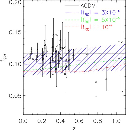
$The evolution of fgas in four models with the same cosmic value of Ωb/Ωm from Planck Collaboration XIII (2015). The models are, respectively, ΛCDM (black solid line), and Hu–Sawicki n = 1 f(R) model with $|\bar{f}_{R0}|=3\times 10^{-5}$ (blue dotted line), 5 × 10−5 (green dashed line) and 10−4 (red dot–dashed line). Black triangles with error bars are the fgas values of the 42 clusters used in Allen et al. (2008, table 3). The blue shaded region denotes the standard deviation around the mean fgas for the model with $|\bar{f}_{R0}|=3\times 10^{-5}$, for illustration, which shows that the theoretical uncertainty is roughly of the same order as current observational errors in fgas; therefore, the constraining power can be further improved if either of these uncertainties is reduced in the future.$

Figure 3.

The evolution of f_gas in four models with the same cosmic value of Ω_b/Ω_m from Planck Collaboration XIII (2015). The models are, respectively, ΛCDM (black solid line), and Hu–Sawicki n = 1 f(R) model with |$|\bar{f}_{R0}|=3\times 10^{-5}$| (blue dotted line), 5 × 10⁻⁵ (green dashed line) and 10⁻⁴ (red dot–dashed line). Black triangles with error bars are the f_gas values of the 42 clusters used in Allen et al. (2008, table 3). The blue shaded region denotes the standard deviation around the mean f_gas for the model with |$|\bar{f}_{R0}|=3\times 10^{-5}$|⁠, for illustration, which shows that the theoretical uncertainty is roughly of the same order as current observational errors in f_gas; therefore, the constraining power can be further improved if either of these uncertainties is reduced in the future.

Open in new tab Download slide

5 DISCUSSION AND CONCLUSIONS

In this paper, we proposed a new cosmological test of gravity, by inferring the cosmic baryon fraction from the apparent gas fractions of massive clusters, and comparing with the results from other, less model-dependent, measurements such as the CMB. In theories with a stronger gravity, the apparent gas fraction is smaller than that in ΛCDM for a fixed Ω_b/Ω_m. Reversely, if the observed value |$f^{\rm obs}_{\rm gas}$| is fixed, we would find a higher value of Ω_b/Ω_m than in GR, that can be inconsistent with the model-independent measurements. Taking the Hu–Sawicki f(R) model as an example: our quick calculation shows that model parameters |$|\bar{f}_{R0}|\sim 5\times 10^{-5}$| are in tension with the gas fraction data of the 42 clusters from Allen et al. (2008), though a more rigorous constraint will be left for future work.

f_gas has been a rather widely used observable (e.g. White et al. 1993), and its power in constraining cosmology – in particular dark energy models – is convincingly demonstrated in various previous works (e.g. Sasaki 1996; Allen et al. 2004, 2008). The inclusion of baryons opens a new dimension for tests of gravity, since ultimately most cosmological observables can be tracked back to lights emitted by interactions involving baryons. In the mean time, the physics of the X-ray-emitting hot gas in massive clusters is relatively clean, making it easier both for the modelling and to use the observational data. As an example, the assumption that gas temperature depends on the gravitational potential and our main conclusions that (i) |$f^\ast _{\rm gas}$| – the true gas fraction – is unchanged with modified gravity while (ii) |$f^{\rm obs}_{\rm gas}$| is changed are supported by hydrodynamical simulations in f(R) gravity (e.g. He & Li 2015). Some uncertainties remain in relating f_gas to Ω_b/Ω_m, but these have been included in the error budget estimate above. Furthermore, within our current state of understanding, slightly changing its modelling (e.g. from Allen et al. 2004 to Allen et al. 2008) does not change results drastically.

Here, we would like to emphasize the use of effective haloes (He et al. 2015) in our analysis. Though the idea has a similar origin as that of the dynamical mass of halo (e.g. Schmidt 2010), there are fundamental differences. Dynamical mass is a certain attribute of a given halo which is defined in the standard way, while effective halo is a completely new way to define and identify haloes. Given an effective halo, all gravitational effect can be calculated from GR, and in particular this means that the way in which f_gas is currently extracted from observational data – and the resulting f_gas results – can be directly used for our purpose. Thus, with a little extra effort from the people who generate a halo catalogue, the analyses of end users can be made much more straightforward, and this provides an efficient bridge between simulators, theorists and observers.

One may naturally wonder about the generality of this method. As a cosmological test, it relies on galaxy clusters being totally or partially unscreened. Because we are talking about massive clusters which tend to be better screened, this test, like most other cosmological ones, will probably not be able to constrain |$\bar{f}_{R0}$| to substantially smaller than the quoted values here. However, it does provide a fairly clean test – with good observational data available – that has the potential to place one of the strongest constraints from cosmology on f(R) gravity. Furthermore, one can always combine f_gas and other observables, such as lensing (Terukina et al. 2014; see Mantz et al. 2014, for an application of combining f_gas and lensing data, amongst others, to constrain cosmology), cluster scaling relations (e.g. Arnold, Puchwein & Springel 2014) and cluster gas pressure profiles (De Martino et al. 2014), to place joint, and likely stronger, constraints. In principle, the test would be more powerful if observational data for smaller galaxy clusters (e.g. those in the mass range 10¹³–10¹⁴ h⁻¹ M_⊙) and galaxy groups are included, because these objects are less screened and so gravity deviates more from GR in general. This, however, requires a better understanding of the feedbacks in different models, which are not well studied so far.

The test can be applied not only to f(R) gravity and the more general chameleon theory, but also to similar models such as dilatons (Brax et al. 2010) and symmetrons (Hinterbichler & Khoury 2010). These models are all featured by a universal coupling of all matter species to a scalar field that effectively enhances the gravity for all particles (at least in unscreened regimes). There are models in which only certain matter species, e.g. dark matter, experiences the scalar coupling: therein, baryons can still feel a different gravity depending on how the dark matter particle mass evolves with time, in which case the proposed test does apply. In addition to these theories, we have mentioned above the DGP, Galileon and K-mouflage models. In the first two classes, the deviations from GR are strongly suppressed inside dark matter haloes (Barreira et al. 2013, 2014a), and so we do not expect the new test to work. For K-mouflage, as is for the so-called non-local gravity (Maggiore & Mancarella 2014; Dirian et al. 2014; Barreira et al. 2014b), there can be a time evolution of Newton's constant inside clusters, making it possible to use this test. However, one needs to bear in mind that in many of these theories the background evolution history is also modified, and that can affect the f_gas test (whether it leads to degeneracies or stronger constraints can only be told by a case-by-case study in the future).

As mentioned earlier, the aim of this paper is to illustrate the main idea of using f_gas as a test of gravity theories, and therefore we have made a simplified estimate and have not quoted any numerical results on the confidence levels of the constrained f_R0. A more complete and rigorous analysis will require one to relax the simplification that all observed clusters share the same mass, radius and concentration, and use the real observational results of these for all clusters. If the cluster mass is obtained from its dynamical effects, we also need to account for the fact that different clusters may have experienced different degrees of screening, and so a more accurate modelling of the screening is needed to compute the cluster mass profile. These will be left for future work. We note that hydrodynamical simulations for modified gravity theories started to appear recently (e.g. Arnold et al. 2014; Hammami et al. 2015, He & Li 2015), and such works will be useful for improving the constraining power of this test in the future.

We thank Sownak Bose, Vince Eke, Claudio Llinares and Gongbo Zhao for discussions and comments. The work has used the DiRAC Data Centric system at Durham University, operated by the Institute for Computational Cosmology on behalf of the STFC DiRAC HPC Facility (www.dirac.ac.uk). This equipment was funded by BIS National E-infrastructure capital grant ST/K00042X/1, STFC capital grant ST/H008519/1, and STFC DiRAC Operations grant ST/K003267/1 and Durham University. DiRAC is part of the National E-Infrastructure. BL acknowledges support by the UK STFC Consolidated Grant No. ST/L00075X/1 and No. RF040335. JHH is supported by the Italian Space Agency (ASI) via contract agreement I/023/12/0. LG acknowledges support from NSFC grants Nos. 11133003 and 11425312, the Strategic Priority Research Program The Emergence of Cosmological Structure of the Chinese Academy of Sciences (No. XDB09000000), MPG partner Group family, and an STFC and Newton Advanced Fellowship.

1

We note here that other observations of Ω_b/Ω_m may depend on the underlying theory of gravity as well, and hence may differ from the constraints in the ΛCDM framework. This must be taken into account when making the above comparisons. For the gravity theory and parameter space that we focus on in this work, the effect on CMB is very weak, and thus we consider that the values of Ω_b/Ω_m inferred from CMB data are the same for the two models.

2

More accurately speaking, effective haloes are identified from the effective density field, ρ_m,eff in equation (20), and standard haloes are identified from the physical density field ρ_m. They do not necessarily share the same physical particles. Here, for simplicity, when talking about the effective and actual masses of some halo, we mean the masses of the effective and standard haloes that would be considered as matched haloes in the two catalogues.

3

Note in equation (22) it is ρ_gas(r)/ρ_gas(0) that is determined by m(r/r_s). The normalization of ρ_gas will then be fixed by the total gas fraction inside the halo.

4

Note that the f(R) models studied here have practically identical CMB power spectra as the ΛCDM model with the same Ω_m and |$\Omega _\Lambda$|⁠. As a result, using CMB data only, the constraints on cosmological parameters such as Ω_m would be the same in all these models. Because of this, the CMB constraints are less model dependent.

REFERENCES

Allen

S. W.

Schmidt

R. W.

Ebeling

H.

Fabian

A. C.

van Speybroeck

L.

2004

MNRAS

353

457

Month:	Total Views:
January 2017	3
February 2017	1
March 2017	1
April 2017	2
May 2017	1
June 2017	4
July 2017	4
August 2017	3
September 2017	2
October 2017	10
November 2017	5
December 2017	2
January 2018	5
March 2018	1
April 2018	2
May 2018	1
July 2018	1
September 2018	1
December 2018	5
February 2019	2
March 2019	2
April 2019	9
May 2019	13
June 2019	18
July 2019	20
August 2019	14
September 2019	10
October 2019	15
November 2019	20
December 2019	21
January 2020	5
February 2020	12
March 2020	6
April 2020	9
May 2020	5
June 2020	2
July 2020	8
August 2020	8
September 2020	5
October 2020	4

Article Contents

Cluster gas fraction as a test of gravity

Abstract

1 INTRODUCTION

2 The f(R) gravity theory

3 CLUSTER GAS FRACTION

3.1 The standard ΛCDM model

3.2 Modified gravity scenarios

4 NUMERICAL EXAMPLES

5 DISCUSSION AND CONCLUSIONS

REFERENCES

Citations

Views

Altmetric

Email alerts

Astrophysics Data System

Citing articles via

Latest

Most Read

Most Cited

This Feature Is Available To Subscribers Only