


Abstract
In anticipation of the Gaia astrometric mission, a sample of spectroscopic binaries is being observed since 2010 with the Spectrograph pour l'Observation des PHénomènes des Intérieurs stellaires et des Exoplanètes (SOPHIE) spectrograph at the Haute-Provence Observatory. Our aim is to derive the orbital elements of double-lined spectroscopic binaries (SB2s) with an accuracy sufficient to finally obtain the masses of the components with relative errors as small as 1 per cent when combined with Gaia astrometric measurements. In order to validate the masses derived from Gaia, interferometric observations are obtained for three SB2s in our sample with F-K components: HIP 14157, HIP 20601 and HIP 117186. The masses of the six stellar components are derived. Due to its edge-on orientation, HIP 14157 is probably an eclipsing binary. We note that almost all the derived masses are a few per cent larger than the expectations from the standard spectral type–mass calibration and mass–luminosity relation. Our calculation also leads to accurate parallaxes for the three binaries, and the Hipparcos parallaxes are confirmed.
1 INTRODUCTION
In a previous paper (Halbwachs et al. 2014), we presented the selection of a sample of double-lined spectroscopic binaries (SB2s) for which it will be possible to derive accurately the masses of the components when the astrometric measurements of the Gaia satellite will be delivered. Our aim is to obtain high-precision radial velocity (RV) measurements in order to derive the minimum masses of the components, |${\cal M}_1 \sin ^3 i$| and |${\cal M}_2 \sin ^3 i$|, where |${\cal M}_1$| and |${\cal M}_2$| are the masses and i is the inclination of the orbital plane on the plane of the sky. The Gaia astrometric measurements of the photocentre of these systems will lead to the derivation of astrometric orbits, including i, and therefore to |${\cal M}_1$| and |${\cal M}_2$|. The RV measurements are obtained through two different programmes: a programme of about 70 SB2s is carried on with the T193 telescope of the Haute-Provence Observatory (OHP) with the SOPHIE spectrograph, and a separate programme of seven SB2s is using the Mercator 1.2 m telescope at the Roque de los Muchachos Observatory (RMO), with the High Efficiency and Resolution Mercator Echelle Spectrograph (HERMES) spectrograph (Raskin et al. 2011).
Despite the high quality that is expected for the Gaia measurements, we know from the reduction of the Hipparcos satellite (ESA 1997; van Leeuwen 2007) that large space astrometric surveys may be prone to systematic errors. The discussion about the reliability of the Hipparcos results is still not closed: recently, Fekel (2015) found an important discrepancy between the parallax he obtained for the system HD 207651 and the parallax given in the Hipparcos 2 catalogue (van Leeuwen 2007), even when the orbital motion is taken into account.
The large variations affecting the basic angle of Gaia will make the verification of the Gaia measurements even more necessary (Mora et al. 2015). Regarding double stars, a good orbit determination with Gaia depends on the measurements at various epochs, and ultimately relies on the application of the point spread function (PSF) calibration, considering the object as a single star. Binaries may then be sensitive to small differences between the position given by the PSF and the position of the actual photocentre. Therefore, an independent derivation of the masses of some stars of our sample is welcome in order to validate our future results.
For these reasons, we obtained interferometric measurements with the Precision Integrated-Optics Near-infrared Imaging ExpeRiment (PIONIER) instrument at the Very Large Telescope Interferometer (VLTI). After one semester, three SB2s were observed over nearly half of their period. Two of these systems are from the OHP programme, and the other is from the RMO programme. HIP 14157 is a couple of chromospherically active K-dwarf stars which was noticed by Fekel, Henry & Alston (2004) for their large minimum masses. HIP 20601 is a Hyades binary star observed by Griffin et al. (1985), and that seems also to have components with masses above expectations. HIP 117186 is an early F-type dwarf from the sample of Nordström et al. (1997).
The obtention of the interferometric observations is described in Section 2. The RV data and the calculation of the SB2 orbital elements are in Section 3. The masses of the six components are derived in Section 4. Our results are used to derive the mass–luminosity relation in the infrared H band, in Section 5, and also to verify the Hipparcos parallaxes, in Section 6. We conclude in Section 7.
2 THE INTERFEROMETRIC OBSERVATIONS
2.1 The observations
We observed our three systems with the four 1.8 m Auxiliary Telescopes of ESO VLTI, using the PIONIER instrument (Berger et al. 2010; Le Bouquin et al. 2011) in the H band on several nights: 2014 October 6–8, 2014 October 17–20, 2014 October 31–November 1, 2014 November 15–17, 2014 December 4–5, 2015 January 27–28 and 2015 February 5–6. For all targets observed in 2014, we used the prism in low resolution (SMALL) which provides a spectral resolving power R ∼ 15, the fringes being sampled over three spectral channels. Mid-December 2014, the detector of PIONIER was changed to the new Revolutionary Avalanche Photodiode Infrared Detector (RAPID) detector, and therefore observations obtained in 2015 were obtained with the new observing mode, sampling the fringes over six spectral channels. The large VLTI configuration A1-G1-K0-J3 was used – except on the nights of 2014 November 15–17 when A1-G1-I1-K0 was used and on 2015 February 5–6 when H0-I1-D0-G1 was used – leading to baselines of 41 (H0-I1), 47 (G1-I1, H1-I1 and K0-I1), 56.8 (K0-J3), 64 (D0-H0), 71.7 (D0-G1 and H0-G1), 80 (A1-G1), 82.5 (D0-I1), 91 (G1-K0), 107 (A1-I1), 129 (A1-K0), 132.4 (G1-J3) and 140 m (A1-J3).
Data reduction and calibration were done in the usual way with the pndrs package presented by Le Bouquin et al. (2011). Each pointing provides six visibilities and four closure phases dispersed over the few spectral channels across the H band.
These interferometric observations were adjusted by a simple binary model. The diameters of the individual components, all smaller than 0.21 mas, are unresolved by our instrumental set-up. The free parameters are thus the separation, the position angle of the secondary with respect to the primary and the flux ratio. The different epochs were mostly adjusted independently. For few epochs, corresponding to small separations or incomplete data set, the flux ratio was imposed following the results obtained at other epochs.
Fitting a binary model to interferometric observations is non-linear and non-convex.1 We used a classical gridding approach to overcome these issues and to find the deepest minimum. We then used a Levenberg–Marquardt algorithm to determine the best-fitting parameters and their covariance matrix. The astrometric error ellipsoid is the on-sky representation of this covariance matrix.
Our results are summarized in Table 1. The positions of the secondary component with respect to the primary are plotted in Fig. 1.
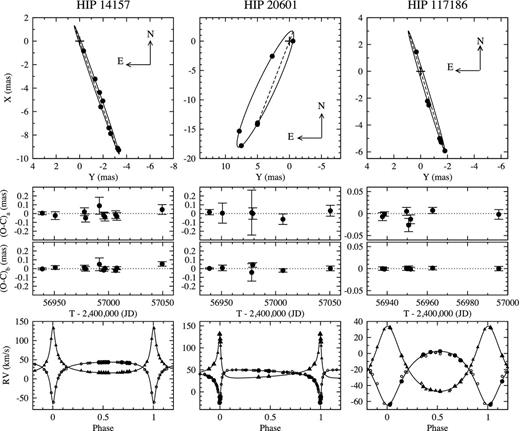
The combined orbits of the three SB2s observed with PIONIER. Upper row: the visual orbits; the node line is in dashes, while the position of the primary is indicated by the cross. Second row: the residuals along the semi-major axis of the error ellipsoid. Third row: the residuals along the semi-minor axis of the error ellipsoid. Last row: the spectroscopic orbits; the circles refer to the primary component, and the triangle to the secondary; the large filled symbols refer to the new RV measurements obtained with HERMES or SOPHIE. For each SB2, the RVs are shifted to the same zero-point.
The interferometric measurements. The column f2/f1 gives the flux ratio between the two components in the infrared H band. ρ is the separation between the components, and θ is the position angle of the secondary with respect to the primary component. σmax and σmin are the semi-major axis and the semi-minor axis of the error ellipsoid, respectively, corrected as indicated in Section 2.2. The last column is the position angle of the semi-major axis of the error ellipsoid. The flux ratios flagged with asterisks were fixed in the fitting procedure.
| MJD | f2/f1 | ρ | θ | σmax | σmin | PA |
|---|---|---|---|---|---|---|
| (mas) | (deg) | (mas) | (mas) | (deg) | ||
| HIP 14157 | ||||||
| 56938.290 | 0.663 | 5.88 | −162.05 | 0.017 | 0.010 | 132 |
| 56950.291 | 0.683 | 3.48 | −157.77 | 0.044 | 0.022 | 118 |
| 56977.272 | 0.676 | 8.31 | −161.43 | 0.044 | 0.026 | 155 |
| 56978.285 | 0.691 | 7.79 | −161.28 | 0.046 | 0.026 | 159 |
| 56991.054 | 0.670* | 0.89 | −158.44 | 0.096 | 0.072 | 110 |
| 56995.109 | 0.688 | 4.69 | −158.73 | 0.039 | 0.015 | 150 |
| 56996.165 | 0.676 | 5.47 | −158.75 | 0.046 | 0.017 | 149 |
| 57006.115 | 0.662 | 9.68 | −160.33 | 0.043 | 0.019 | 153 |
| 57007.140 | 0.664 | 9.87 | −160.19 | 0.043 | 0.017 | 143 |
| 57049.045 | 0.666 | 9.69 | −160.41 | 0.056 | 0.026 | 129 |
| HIP 20601 | ||||||
| 56938.367 | 0.402 | 3.72 | +133.73 | 0.030 | 0.0067 | 139 |
| 56950.348 | 0.400* | 0.55 | −89.55 | 0.11 | 0.032 | 150 |
| 56977.353 | 0.400* | 14.79 | +160.44 | 0.25 | 0.099 | 148 |
| 56978.321 | 0.400* | 15.06 | +160.61 | 0.065 | 0.027 | 149 |
| 57006.187 | 0.402 | 19.32 | +157.20 | 0.060 | 0.020 | 157 |
| 57050.051 | 0.387 | 17.24 | +153.02 | 0.062 | 0.027 | 162 |
| HIP 117186 | ||||||
| 56937.179 | 0.440 | 2.28 | −166.93 | 0.0090 | 0.0036 | 8 |
| 56938.210 | 0.440 | 2.59 | −166.40 | 0.0045 | 0.0027 | 163 |
| 56949.162 | 0.434 | 5.20 | −164.20 | 0.0086 | 0.0036 | 139 |
| 56950.187 | 0.437 | 5.35 | −163.79 | 0.015 | 0.0050 | 134 |
| 56951.189 | 0.454 | 5.50 | −163.84 | 0.0099 | 0.0036 | 141 |
| 56962.137 | 0.430 | 6.20 | −163.09 | 0.0072 | 0.0036 | 141 |
| 56995.017 | 0.446 | 1.48 | +12.55 | 0.011 | 0.0045 | 168 |
2.2 Verification and correction of the uncertainties
Reliable uncertainties are needed to derive masses from apparent positions and from RV measurements. This point is especially important hereafter, since several parameters in the common solution leading to the masses are coming as well from the interferometric observations as from the spectroscopic ones. This applies to the period P, the eccentricity e, the epoch of the periastron T0 and the periastron longitude ω. Overestimating the uncertainties of the interferometric observations would lead to underestimating the weights of these observations and to exaggerate the contribution of the RV in the derivation of these terms, and vice versa.
To verify the uncertainties, the ‘visual’ binary (VB) orbit of the star is derived. Computing a visual orbit consists in searching seven unknowns: the period, P, the eccentricity, e, the epoch of the periastron, T0, and the Thiele–Innes elements A, B, F, G. Therefore, a minimum of eight observations is needed to derive these terms and to estimate their errors. Since a relative position is a two-dimensional observation, this corresponds to four interferometric observations. For the least observed star, which is HIP 20601, we have six interferometric observations, resulting in 5 degrees of freedom in the derivation of the orbit. This is sufficient to allow the verification of the error estimations.
It appears that, when the uncertainties provided by the PIONIER reduction are taken into account, F2 is systematically negative. This indicates that these uncertainties are overestimated. In order to keep the relative weights of the observations, the uncertainties of the positions of any star are divided by the same coefficient, in order to have F2 = 0. The uncertainties σmin and σmax in Table 1 are thus obtained. It is worth noticing that they are similar to the errors expected for Gaia (Perryman 2005; Eyer et al. 2015).
3 THE RVS AND THE SB2 ORBITS
3.1 Existing RV measurements
RV measurements are obtained from the SB9 catalogue (Pourbaix et al. 2004), which is regularly updated and accessible online.2 Primarily, the spectroscopic orbits of these stars were derived assigning weights to the measurements of the primary and of the secondary component. Since our purpose is to derive masses not only from these measurements, but also from new RV measurements and from interferometric observations, it is necessary to convert these weights to reliable uncertainties.
To evaluate the uncertainty of the RV of any component, the single-lined orbit of the star is derived. The weights of the RV measurements are transformed to uncertainties in order to get an SB1 orbit with F2 = 0. It is worth noticing that this method is similar in its principle to the usual approach consisting in taking for the uncertainty the standard deviation of the residuals of the RV. However, it is much more reliable and it leads to uncertainties significantly larger.
When the RV uncertainties are obtained for both components, the SB2 orbit is derived, and F2 is calculated again. A correction coefficient is applied to have at the end an SB2 orbit again with F2 = 0. This method leads to the following results.
For HIP 14157, the uncertainty of the RV measured by Fekel et al. (2004) is 0.582 and 0.677 km s−1 for the primary and for the secondary component, respectively.
The standard procedure requires an adaptation for the treatment of the RV measurements provided by Griffin et al. (1985) for HIP 20601. No weights are indicated by the authors, but 7 of the 63 measurements of the primary component are flagged as uncertain, and the secondary component received only 4 RV measurements. We assign 0.843 km s−1 to the uncertainty of the 56 ‘not uncertain’ RV measurements, in order to get an SB1 orbit with F2 = 0. The uncertainty of the ‘uncertain’ primary RV is then 1.504 km s−1, in order to still have F2 = 0 for the SB1 orbit of the primary component. The uncertainty of the RV of the secondary component is then 3.000 km s−1, in order to have F2 = 0 for the SB2 orbit of the binary.
For HIP 117186, the uncertainty of the RV measured by Nordström et al. (1997) is 1.837 and 1.487 km s−1 for the primary and for the secondary component, respectively.
The sets of RV of the three stars are further completed with high-accuracy measurements recently obtained.
3.2 New RV measurements
3.2.1 RVs from the HERMES spectrograph
HIP 14157 received eight RV measurements between 2015 January and August. The fibre-fed HERMES spectrograph covers the whole wavelength range from 380 to 900 nm at a resolving power of ∼86 000. A python-based pipeline extracts a wavelength-calibrated and a cosmic ray-cleaned spectrum. A restricted region, covering the range 478.11–653.56 nm (orders 55–74), was used to derive a cross-correlation function (CCF) with a spectral mask constructed from an Arcturus spectrum and containing 2103 useful spectral lines. A spectrum with a signal-to-noise ratio of 15 is usually sufficient to obtain a CCF with a well-pronounced maximum.
RVs are determined from a Gaussian fit to the core of the CCF with an internal precision of a few m s−1. The most important external source of error is the varying atmospheric pressure in the spectrograph room (see fig. 9 of Raskin et al. 2011), which is largely eliminated by the arc spectra taken for wavelength calibration. The long-term stability (years) of the resulting RVs is checked with RV standard stars from Udry, Mayor & Queloz (1999). Their standard-deviation distribution peaks at σRV = 55 m s−1, which we adopt as the typical RV uncertainty for such relatively bright single stars. The RV standard stars have also been used to tie the HERMES RVs to the IAU standard system.
For an SB2 system, the reduction process leads to estimations of the uncertainties of the RV which are obviously underestimated, due to the pollution of the spectrum of each component by that of the other one. This appears clearly when the orbital elements are derived from the eight HERMES observations of HIP 14157: the goodness of fit of the SB2 solution is as large as F2 = 17.3, and the standard deviations of the residuals are 0.138 and 0.219 km s−1, respectively. We assume then that the ratio of the true uncertainties is σRV2/σRV1 = 1.59. The uncertainties are then increased, by adding quadratically a noise depending on the component, until we have F2 = 0. This condition is fulfilled with the noises 0.187 and 0.298 km s−1, respectively. This method is a bit different from the one applied above to derive the uncertainties of the previously published measurements, since the correction of the uncertainties is not done separately for each component. However, it is more suitable for an SB2 with few observations. The RVs of the components of HIP 14157 and the uncertainties thus obtained are listed in Table 3.
3.2.2 Derivation of RV from SOPHIE spectra with todmor
HIP 20601 and HIP 117186 received 12 and 7 SOPHIE spectra, respectively, between 2010 December and 2014 December. The RVs of the components are derived using the two-dimensional correlation algorithm todcor (Zucker & Mazeh 1994; Zucker et al. 2004), as explained hereafter.
The todcor algorithm calculates the cross-correlation of an SB2 spectrum and two best-matching stellar atmosphere models, one for each component of the observed binary system. This two-dimensional cross-correlation function (2D-CCF) is maximized at the RVs of both components. The multi-order version of TwO-Dimensional CORrelation (todcor), named todmor (Zucker et al. 2004), determines the RVs of both components from the gathering of the 2D-CCF obtained from each order of the spectrum.
All SOPHIE multi-order spectra are deblazed, then pseudo-continuum normalized using a p-percentile filter (Hodgson et al. 1985). The percentile p = 0.5 selects the median among all flux values contained within the filter's window; any p > 0.5 selects flux with value larger than the median. The percentile p and the width w of the filtering window are chosen so that the resulting normalized spectra are as flat as possible, while not altering the depth and shape of any lines. These constraints led us to choose for both targets w ∼ 1300 pixels (∼33 Å); the width of one SOPHIE order is about 4000 pixels (∼100 Å); 33 Å is about twice the full width at half-maximum for a Balmer line of early-type stars and for Ca ii lines of late-type stars. The value of p was determined independently for each order by maximizing the two-dimensional cross-correlation.
We determined for the two components of each binary best-matching atmospheric models from the PHOENIX library (Husser et al. 2013). For consistency, we also applied a p-percentile filter on the spectra of the models, with p = 0.99 and the same window's width as for HIP 117186 and HIP 20601 spectra, of ∼1300 pixels. On those spectra for which both peaks of the SB2 components are well separated, we optimized the 2D-CCF varying the effective temperature, the stellar rotation's v sin ir, the metallicity and the surface gravity's log g of both components.
The derived values of the stellar parameters are given for both components in Table 2. For HIP 117186, only one spectrum had large enough separation between the primary and secondary peaks, namely the spectrum observed at periastron passage. For HIP 20601, all spectra gave very consistent results, up to 5 and 100 K in effective temperature for the primary and secondary, respectively, 0.03 and 0.4 in log g, 0.2 and 0.6 km s−1 in v sin ir, 0.01 in metallicity and 0.01 in flux ratio. However, the individual uncertainties are much larger than these scatter values, so we give here the average individual uncertainties divided by the square root of the number of spectra used for deriving the parameters, namely |$\sqrt{N_{\rm spec}}$|.
The stellar parameters determined by optimization of the 2D-CCF obtained with todmor. At the bottom, Nspec is the number of spectra used to derive the parameter values.
| Parameters | HIP 20601 | HIP 117186 |
|---|---|---|
| Teff,1 (K) | 5600 ± 90 | 6580 ± 230 |
| log g1 (dex) | 4.43 ± 0.26 | 3.8 ± 0.6 |
| v1 sin ir 1(km s− 1) | 4.6 ± 1.0 | 43 ± 13 |
| Teff,2 (K) | 4550 ± 550 | 6550 ± 490 |
| log g2 (dex) | 4.76 ± 0.92 | 4.32 ± 0.82 |
| v2 sin ir 2(km s− 1) | <2 | 13 ± 11 |
| m/H (dex) | − 0.38 ± 0.10 | − 0.35 ± 0.24 |
| α (flux ratio) | 0.106 ± 0.006 | 0.374 ± 0.151 |
| Nspec | 4 | 1 |
Finally, we applied todcor to all multi-order spectra of each target and determined the RVs of both components. We discarded several orders of the spectra of HIP 20601 and HIP 117186, which were strongly affected by telluric lines (orders 31, 34, 36 and 39). At a given exposure, for each of the selected orders, we calculated a 2D-CCF, from which we derived the maximizing values of RVs for the primary and the secondary.
For each target, there are systematic order-to-order variations of the RV measurements, different for each SB2 component. These systematics come from signal-to-noise, number of atomic lines available and discrepancies of the models with the real spectrum; they are specific to each component and each order. To estimate them, we first calculated for each exposure the residuals of the velocities derived for all individual order around the median velocity; then we considered the residuals obtained for all exposures at an individual order, and calculated the systematic shift for this order as the median of the residuals. We estimated as well a measurement error for each order from the scatter of its residuals about the systematics.
Then, we determined at all epochs the RVs of the primary and the secondary and their uncertainties from the weighted average and the square root of the weighted variance of the corrected order-by-order velocities.
The uncertainties of the RV measurements thus obtained need to be verified, and possibly corrected, since the method of calculation leads to overestimating the errors. Again, the verification is based on F2, and when a correction is necessary, it is done in order to obtain F2 = 0. For HIP 20601, we have 12 RV measurements for each component. We derive the six parameters of each SB1 orbit, and F2 is obtained with 6 degrees of freedom. For the primary and for the secondary component, we obtain F2 = −1.63 and −2.43, respectively. These small values clearly confirm that the uncertainties are too large for both components. They are multiplied by 0.554 and 0.369, respectively, in order to have F2 = 0. When the SB2 orbit is derived with the corrected uncertainties, F2 = 0.32. Although this value seems quite acceptable, we apply an additional correction factor of 1.058, in order to have F2 = 0 for the SB2 orbit coming from our measurements, as we did for the SB2 orbit obtained from previously published measurements, in Section 3.1.
We have only seven RV measurements for each component of HIP 117186. This number is sufficient to derive the SB1 orbits, but, with only 1 degree of freedom, the method applied to HIP 20601 is not sufficiently robust to lead to reliable uncertainties. Therefore, we consider only the SB2 orbit, which is derived with 6 degrees of freedom. We have F2 = −0.81, and we correct the uncertainties by multiplying them by 0.766. After this correction, we verify that both SB1 orbits have acceptable values of F2: we find F2 = −0.13 and −0.77, respectively.
The RVs and the uncertainties finally derived are in Table 3.
The new RVs obtained from HERMES (HIP 14157) or from SOPHIE (HIP 20601 and HIP 117186). The uncertainties are revised as explained in the text.
| BJD | RV1 | σRV 1 | RV2 | σRV 2 |
|---|---|---|---|---|
| −2400000 | (km s−1) | (km s−1) | (km s−1) | (km s−1) |
| HIP 14157 | ||||
| 56672.3674 | 43.525 | 0.189 | 17.222 | 0.300 |
| 57052.4032 | 43.272 | 0.189 | 16.272 | 0.301 |
| 57053.3496 | 43.454 | 0.189 | 16.047 | 0.300 |
| 57054.3817 | 43.694 | 0.188 | 15.918 | 0.300 |
| 57055.3393 | 43.869 | 0.189 | 15.790 | 0.300 |
| 57056.3651 | 43.881 | 0.189 | 15.774 | 0.300 |
| 57237.7366 | 42.125 | 0.188 | 18.107 | 0.300 |
| 57238.7311 | 41.513 | 0.189 | 18.983 | 0.301 |
| HIP 20601 | ||||
| 55532.4785 | 25.8044 | 0.0423 | 62.9854 | 0.1795 |
| 56243.5140 | 46.9337 | 0.0176 | 34.5268 | 0.2933 |
| 56323.2404 | −24.2847 | 0.0196 | 130.7605 | 0.1366 |
| 56323.3136 | −24.7068 | 0.0185 | 131.1920 | 0.1084 |
| 56323.3628 | −24.9163 | 0.0198 | 131.5768 | 0.1179 |
| 56323.4538 | −25.1587 | 0.0193 | 131.8981 | 0.1920 |
| 56323.5102 | −25.2156 | 0.0224 | 132.0942 | 0.1792 |
| 56324.2438 | −16.4490 | 0.0251 | 119.8076 | 0.1136 |
| 56324.4318 | −12.0964 | 0.0125 | 114.1730 | 0.1463 |
| 56324.4718 | −11.1097 | 0.0199 | 112.7543 | 0.2391 |
| 56619.5265 | 33.7880 | 0.0315 | 52.4828 | 0.3178 |
| 57009.4242 | 48.1646 | 0.0224 | 33.0725 | 0.2846 |
| HIP 117186 | ||||
| 55864.3650 | −8.5826 | 0.8246 | −35.8419 | 0.2292 |
| 56147.5270 | −64.0310 | 0.8484 | 32.1576 | 0.1751 |
| 56243.3282 | −34.8861 | 1.4155 | −3.0639 | 0.2020 |
| 56525.5154 | 1.6961 | 0.4467 | −45.6927 | 0.1320 |
| 56619.4355 | 2.7450 | 0.7522 | −47.3041 | 0.1390 |
| 56889.5626 | −2.5384 | 0.7092 | −41.1859 | 0.1439 |
| 56948.4278 | −1.3476 | 0.7158 | −41.6893 | 0.1622 |
3.3 The SB2 orbits
We compute the SB2 orbits, taking into account simultaneously the existing and the new measurements. In addition to the usual parameters of an SB2 orbit, we introduce three offsets of the RV measurements: dn−p, the offset between the new measurements and the published ones, and |$d^p_{2-1}$| and |$d^n_{2-1}$|, the offsets between the RV of the secondary components and the RV of the primary components, for the published and for the new measurements. The systemic velocity, V0, is derived in the system of the new RV measurements of the primary component.
For HIP 14157 and HIP 20601, F2 = −0.041 and −0.16, respectively, indicating that both sets of measurements are quite compatible. For HIP 117186, F2 = 0.78, since some discrepancies appear between the SB2 orbit derived from the new measurements and the preceding one; the most important is the mass ratio, which is 0.771 ± 0.021 with the previously published measurements and 0.844 ± 0.012 with our observations. Nevertheless, the SB2 orbit obtained from both sets of RVs is basically indistinguishable from the one derived from our measurements alone, but the period is much more accurate, thanks to the extension of the timespan covered by the observations. The new SB2 orbits are presented in Table 4.
The orbital elements of the three stars, derived from both the previously existing RV measurements and from the new ones. The minimum masses and minimum semi-major axes are derived from the true period (Ptrue = P × (1 − V0/c)).
| HIP | P | T0(BJD) | e | V0 | ω1 | K1 | |${\cal M}_1 \sin ^3 i$| | a1sin i | N1 | dn−p | σ(O1 − C1)p, n |
|---|---|---|---|---|---|---|---|---|---|---|---|
| K2 | |${\cal M}_2 \sin ^3 i$| | a2sin i | N2 | |$d^p_{2\!-\!1},d^n_{2\!-\!1}$| | σ(O2 − C2)p, n | ||||||
| (d) | 2400000+ | (km s−1) | (o) | (km s−1) | (M⊙) | (106 km) | (km s−1) | (km s−1) | |||
| 14157 | 43.320 58 | 51487.495 | 0.7602 | 30.751 | 174.60 | 54.31 | 0.980 | 21.014 | 23+8 | 0.343 | 0.555, 0.142 |
| ±0.000 49 | ±0.012 | ±0.0015 | ±0.094 | ±0.22 | ±0.29 | ±0.010 | ±0.094 | ±0.176 | |||
| 60.45 | 0.8801 | 23.39 | 23+8 | 0.434, −0.167 | 0.636, 0.312 | ||||||
| ±0.34 | ±0.0089 | ±0.11 | ±0.201, ±0.170 | ||||||||
| 20601 | 156.380 19 | 56636.6716 | 0.851 47 | 41.623 | 202.042 | 37.342 | 0.9060 | 42.101 | 63+12 | −0.442 | 0.951, 0.015 |
| ±0.000 27 | ±0.0027 | ±0.000 25 | ±0.014 | ±0.089 | ±0.017 | ±0.0037 | ±0.025 | ±0.112 | |||
| 50.390 | 0.6714 | 56.81 | 4+12 | 0.416, 0.071 | 2.53, 0.143 | ||||||
| ±0.088 | ±0.0018 | ±0.10 | ±1.531, ±0.136 | ||||||||
| 117186 | 85.8266 | 56403.36 | 0.3362 | −19.59 | 178.75 | 33.40 | 1.627 | 37.12 | 19+7 | 1.121 | 2.14, 0.799 |
| ±0.0017 | ±0.27 | ±0.0035 | ±0.32 | ±0.86 | ±0.39 | ±0.028 | ±0.44 | ±0.527 | |||
| 40.31 | 1.348 | 44.81 | 19+7 | 0.519, −0.967 | 1.41, 0.107 | ||||||
| ±0.18 | ±0.033 | ±0.23 | ±0.558, ±0.411 |
4 THE MASSES
4.1 Derivation of the masses
The masses of the components are directly derived from the interferometric and from the RV measurements, taken into account simultaneously. However, we increase the RV uncertainties of HIP 117186 by 1.088, which would lead to an SB2 orbit with F2 = 0. This operation increases the relative weights of the interferometric measurements in the derivation of the combined orbit. The solution consists of up to 13 independent parameters, which are the orbital parameters P, T0, e, V0, ω1, i, Ω1, the masses |${\cal M}_1$|, |${\cal M}_2$|, the trigonometric parallax ϖ, and also the RV offsets dn − p, |$d^p_{2-1}$| and |$d^n_{2-1}$|. It is worth noticing that we prefer to directly obtain |${\cal M}_1$|, |${\cal M}_2$| and ϖ, rather than the observational parameters K1, K2 and a, the apparent semi-major axis of the interferometric orbit. The advantage of this method is that it leads directly to the uncertainties of the masses and of the parallax, in place of the uncertainties on K1, K2 and a when the latter parameters are obtained from the combined interferometric and spectroscopic observations. The parameters of the combined solutions are presented in Table 5. The uncertainties of masses range between 0.0019 and 0.034 M⊙, and the relative errors range between 0.26 and 2.4 per cent. This is similar to the accuracies expected using the Gaia astrometry.
The combined VB+SB2 solutions. For consistency with the SB orbits and with the forthcoming astrometric orbit, ω and Ω both refer to the motion of the primary component.
| HIP 14157 | HIP 20601 | HIP 117186 | |
|---|---|---|---|
| P (d) | 43.320 32 | 156.380 20 | 85.8238 |
| ±0.000 13 | ±0.000 26 | ±0.0012 | |
| T0 (BJD−2400000) | 51487.5005 | 56636.6713 | 56402.576 |
| ±0.0079 | ±0.0027 | ±0.072 | |
| e | 0.7594 | 0.851 48 | 0.327 02 |
| ±0.0010 | ±0.000 25 | ±0.000 68 | |
| V0 (km s−1) | 30.743 | 41.623 | −19.89 |
| ±0.091 | ±0.014 | ±0.33 | |
| ω1 (o) | 174.69 | 202.026 | 176.07 |
| ±0.17 | ±0.086 | ±0.32 | |
| Ω1(o; eq. 2000) | 19.141 | 340.526 | 16.928 |
| ±0.082 | ±0.058 | ±0.047 | |
| i (o) | 92.24 | 103.138 | 88.054 |
| ±0.18 | ±0.077 | ±0.043 | |
| aa (mas) | 5.810 | 11.339 | 4.677 |
| ±0.034 | ±0.068 | ±0.032 | |
| |${\cal M}_1$| (M⊙) | 0.982 | 0.9808 | 1.686 |
| ±0.010 | ±0.0040 | ±0.021 | |
| |${\cal M}_2$| (M⊙) | 0.8819 | 0.7269 | 1.390 |
| ±0.0089 | ±0.0019 | ±0.034 | |
| ϖ (mas) | 19.557 | 16.702 | 8.445 |
| ±0.078 | ±0.037 | ±0.075 | |
| nVLTI × 2 | 20 | 12 | 14 |
| σ(o−c) VLTI (mas) | 0.035 | 0.031 | 0.0084 |
| nRV1 | 23+8 | 63+12 | 19+7 |
| σ(o−c) RV1 (km s−1) | 0.562, 0.156 | 0.952, 0.015 | 2.40, 0.89 |
| nRV2 | 23+8 | 4+12 | 19+7 |
| σ(o−c) RV2 (km s−1) | 0.646, 0.282 | 2.54, 0.143 | 1.11, 0.23 |
| dn−p (km s−1) | 0.323 | −0.441 | 0.822 |
| ±0.172 | ±0.111 | ±0.563 | |
| |$d^p_{2-1}$| (km s−1) | 0.408 | 0.436 | 0.549 |
| ±0.198 | ±1.513 | ±0.606 | |
| |$d^n_{2-1}$| (km s−1) | −0.149 | 0.077 | −0.184 |
| ±0.161 | ±0.135 | ±0.335 |
aThe uncertainty refers to the VB solution.
4.2 Notes on individual objects
HIP 14157. This system is extensively discussed by Fekel et al. (2004), who pointed out that the primary is a BY Dra variable star with a variability amplitude around 0.02 mag. Due to an inclination almost edge-on, the masses of the components are close to the minimum masses that they found. We confirm then that the mass of the K2-K3 V secondary component is 0.882 M⊙. This is larger than the canonical value, which is between 0.67 M⊙ (for a K5 V star) and 0.79 M⊙ (for a K0 V star) according to Cox (2000). Such discrepancy is not surprising, but known since a while, since Griffin et al. (1985) and references therein already pointed out that the real masses of K-type stars are usually 15 per cent larger than the canonical values. In a similar way, we find that the primary component is too heavy for a K0 V star. The minimum projected separation between the components is only 0.090 mas, corresponding to 0.99 R⊙. Since Fekel et al. estimated the stellar radii R1 = 0.99 and R2 = 0.76 R⊙, the system is very likely an eclipsing one.
HIP 20601. The star is a candidate member of the Hyades cluster (Perryman et al. 1998; de Bruijne, Hoogerwerf & de Zeeuw 2001). Griffin et al. (1985) estimated that the spectral types of the components are probably G6 and K5, in good agreement with our estimates of the effective temperatures. As a consequence, the masses are around 7 per cent larger than the canonical values listed in Cox (2000).
HIP 117186. The effective temperatures of the components correspond to spectral types around F5, and the canonical masses are around 1.4. This corresponds well to the mass of the secondary component, but is around 20 per cent percent less than the mass of the primary component.
5 THE INFRARED MASS–LUMINOSITY RELATION
The data derived from PIONIER observations include the flux ratios f2/f1 which are listed in Table 1. The photometric band is similar to the infrared H band of 2MASS (Skrutskie et al. 2006), and, for each binary, we derive the mean value of the magnitude difference, ΔH, and its standard error. The total H magnitudes of the binaries are taken from Cutri et al. (2003), and the individual absolute H magnitudes of the components are then computed, using the parallaxes from Table 5. The results are given in Table 6.
| HIP 14157 | HIP 20601 | HIP 117186 | |
|---|---|---|---|
| Htot | 6.629 ± 0.029 | 7.209 ± 0.047 | 6.252 ± 0.031 |
| ΔH | 0.429 ± 0.017 | 0.999 ± 0.016 | 0.891 ± 0.020 |
| MH 1 | 3.645 ± 0.031 | 3.687 ± 0.047 | 1.281 ± 0.037 |
| MH 2 | 4.073 ± 0.032 | 4.686 ± 0.049 | 2.172 ± 0.039 |
| HIP 14157 | HIP 20601 | HIP 117186 | |
|---|---|---|---|
| Htot | 6.629 ± 0.029 | 7.209 ± 0.047 | 6.252 ± 0.031 |
| ΔH | 0.429 ± 0.017 | 0.999 ± 0.016 | 0.891 ± 0.020 |
| MH 1 | 3.645 ± 0.031 | 3.687 ± 0.047 | 1.281 ± 0.037 |
| MH 2 | 4.073 ± 0.032 | 4.686 ± 0.049 | 2.172 ± 0.039 |
| HIP 14157 | HIP 20601 | HIP 117186 | |
|---|---|---|---|
| Htot | 6.629 ± 0.029 | 7.209 ± 0.047 | 6.252 ± 0.031 |
| ΔH | 0.429 ± 0.017 | 0.999 ± 0.016 | 0.891 ± 0.020 |
| MH 1 | 3.645 ± 0.031 | 3.687 ± 0.047 | 1.281 ± 0.037 |
| MH 2 | 4.073 ± 0.032 | 4.686 ± 0.049 | 2.172 ± 0.039 |
| HIP 14157 | HIP 20601 | HIP 117186 | |
|---|---|---|---|
| Htot | 6.629 ± 0.029 | 7.209 ± 0.047 | 6.252 ± 0.031 |
| ΔH | 0.429 ± 0.017 | 0.999 ± 0.016 | 0.891 ± 0.020 |
| MH 1 | 3.645 ± 0.031 | 3.687 ± 0.047 | 1.281 ± 0.037 |
| MH 2 | 4.073 ± 0.032 | 4.686 ± 0.049 | 2.172 ± 0.039 |
The masses and the absolute H magnitudes of the six components are plotted on a mass–luminosity diagram in Fig. 2. The mass–luminosity relation of Henry & McCarthy (1993) is also shown for comparison. Although the masses of our stars are within the uncertainties of the canonical relation, they are in excess by around 8 per cent when Habs is between 3.6 and 4.7 mag.
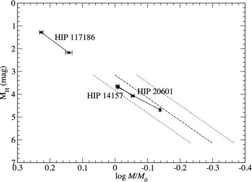
The mass–luminosity diagram in the infrared H band. The relation of Henry & McCarthy (1993) is in dashes, with limits in dotted lines.
6 VERIFICATION OF THE HIPPARCOS PARALLAXES
The elements of the combined solutions presented in Table 5 include parallaxes with errors between 0.037 and 0.078 mas. They are roughly 10 times better than the errors of the parallaxes coming from Hipparcos. However, in the Hipparcos 2 catalogue, the parallaxes of these stars were derived through the single-star (SS) model, ignoring that they are binaries. As a consequence, a discrepancy between our parallaxes and the Hipparcos ones could be due to a reduction based on the use of the SS model, and not to errors in the Hipparcos transits. In order to check the reliability of Hipparcos itself, we first computed the corrections of the Hipparcos 2 parallaxes. For that purpose, the residuals of any SS solution were input in the computation of an astrometric orbital (AO) solution. However, except for the astrometric semi-major axis, a0, all the orbital elements were fixed on the values already obtained. The new parallaxes, ϖAO, are listed in Table 7, with a0 and the goodness of fit of the new solution, F2 AO. The uncorrected parallax and the related goodness of fit, F2 SS, are indicated for comparison. F2 is always ameliorated when the orbital motion is taken into account, and a0 is always smaller than twice its uncertainty. Therefore, it would not have been possible to detect the orbital motion from Hipparcos alone.
The Hipparcos 2 parallaxes, before and after taking into account the orbital motion (ϖSS and ϖAO, respectively). a0 is the semi-major axis of the photocentric orbit derived from Hipparcos data.
| HIP 14157 | HIP 20601 | HIP 117186 | |
|---|---|---|---|
| ϖSS (mas) | 19.78 ± 1.10 | 15.20 ± 1.35 | 6.94 ± 0.57 |
| F2 SS | 0.69 | −0.21 | 2.24 |
| ϖAO (mas) | 19.10 ± 1.09 | 14.84 ± 1.41 | 7.93 ± 0.64 |
| a0 (mas) | 3.06 ± 1.54 | 2.45 ± 1.40 | 1.07 ± 0.48 |
| F2 AO | 0.399 | −0.42 | 2.03 |
| HIP 14157 | HIP 20601 | HIP 117186 | |
|---|---|---|---|
| ϖSS (mas) | 19.78 ± 1.10 | 15.20 ± 1.35 | 6.94 ± 0.57 |
| F2 SS | 0.69 | −0.21 | 2.24 |
| ϖAO (mas) | 19.10 ± 1.09 | 14.84 ± 1.41 | 7.93 ± 0.64 |
| a0 (mas) | 3.06 ± 1.54 | 2.45 ± 1.40 | 1.07 ± 0.48 |
| F2 AO | 0.399 | −0.42 | 2.03 |
The corrected Hipparcos parallaxes are compared to our parallaxes in Fig. 3. For HIP 14157 and HIP 117186, the agreement is less than the standard error. For HIP 20601, the difference is (1.86 ± 1.41) mas, i.e. 1.3 times the standard error. This is still rather good agreement, and it seems that the discrepancy found by Fekel (2015) for HD 207651 is due to peculiarities, such as the presence of a third star.
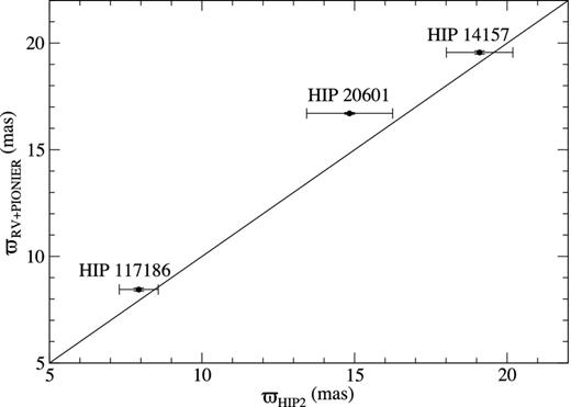
Comparison of the parallaxes derived in the combined solution with the Hipparcos2 parallaxes corrected for the orbital motion.
7 CONCLUSION
We have combined interferometric observations performed with the VLTI with RVs in order to derive the masses of the components of three binary stars. Thanks to the exquisite accuracy of the PIONIER observations, but also to the fact that the orbits are all close to edge-on, the accuracy of the masses thus obtained is between 0.26 and 2.4 per cent. This is less than the 3 per cent limit applied by Torres, Andersen & Giménez (2010) when they set up their list of accurate masses. This is also close to the uncertainties that we expect to obtain combining the RV measurements with Gaia astrometry.
Five of the six masses are a few per cent larger than the expectations coming from the standard spectral type–mass calibration, confirming Griffin et al. (1985). The masses below 1 M⊙ are also around 8 per cent larger than the masses derived from the mass–luminosity relation of Henry & McCarthy (1993), although they are within their error interval. One of our star (HIP 14157) should be observed as an eclipsing binary; this would confirm the small inclination that we have found, and therefore improve the accuracy of the masses, but it would also make possible the estimation of the radii of the components.
The parallaxes are derived at the same time as the orbital elements of the binaries, with an accuracy much better than that of the Hipparcos 2 catalogue. The reliability of the Hipparcos parallaxes is confirmed.
This project was supported by the French INSU-CNRS ‘Programme National de Physique Stellaire’ and ‘Action Spécifique Gaia’. PIONIER is funded by the Université Joseph Fourier (UJF), the Institut de Planétologie et d'Astrophysique de Grenoble (IPAG) and the Agence Nationale pour la Recherche (ANR-06-BLAN-0421, ANR-10-BLAN-0505, ANR-10-LABX56). The integrated optics beam combiner is the result of a collaboration between IPAG and CEA-LETI based on CNES R&T funding. The HERMES spectrograph is supported by the Fund for Scientific Research of Flanders (FWO), the Research Council of KU Leuven, the Fonds National de la Recherche Scientifique (F.R.S.-FNRS), Belgium, the Royal Observatory of Belgium, the Observatoire de Genève, Switzerland and the Thüringer Landessternwarte Tautenburg, Germany. We are grateful to the staff of the Haute-Provence Observatory, and especially to Dr F. Bouchy, Dr H. Le Coroller, Dr M. Véron and the night assistants, for their kind assistance. We warmly thank Dr C. Soubiran for her helpful advices. This research has received funding from the European Community's Seventh Framework Programme (FP7/2007-2013) under grant agreement numbers 291352 (ERC). This work made use of the Smithsonian/NASA Astrophysics Data System (ADS) and of the Centre de Donnees astronomiques de Strasbourg (CDS).
Based on observations performed at the Observatoire de Haute-Provence (CNRS), France.
Based on observations performed with the HERMES spectrograph at the Roque de los Muchachos Observatory.
Based on data obtained with the ESO Very Large Telescope under programme 094.D-0624, 094.C-0884, 094.C-0175 and 094.C-0397.
Broadly speaking, a convex optimization means that there is only one optimal solution, which is therefore globally optimal, i.e. a local minimum is a global one. This is not the case when adjusting a binary model to interferometric observations, as we need to cover the full range of parameters to determine the position of the global minimum.
REFERENCES
ESA
