Non-linearity and environmental dependence of the star-forming galaxies main sequence Free

Abstract

1 INTRODUCTION

The so-called main sequence (MS) of star-forming galaxies is a tight correlation between the star formation rates (SFRs) and the stellar masses of the bulk of the star-forming galaxy population. The MS appears to hold at least over the past 10 Gyr (Daddi et al. 2007; Elbaz et al. 2007; Noeske et al. 2007; Peng et al. 2010; Whitaker et al. 2012, 2014). The zero-point of this relation evolves with cosmic time such that the level of star formation (SF) activity was much higher in the past. Indeed, there is an uncontroversial steep decline in the cosmic star formation history by a factor of 10 since z ∼ 1, after a peak of activity around z ∼ 1–2 (Lilly et al. 1996; Madau, Pozzetti & Dickinson 1998; Le Floc'h et al. 2005; Hopkins et al. 2006). Aside from the normalization, the slope and the dispersion of the relation are still quite uncertain. The measurement of the slope and dispersion vary widely in the literature, ranging between 0.2–1.2 for the slope and 0.3–0.6 for the dispersion (see Speagle et al. 2014 and references therein). Most of the uncertainty is due either to biases introduced by the selection criteria used to identify the star-forming galaxy population, SFR indicators, method of fitting (mean, median, mode) or because the relation is not linear but its slope varies at different mass scales. Indeed, Whitaker et al. (2014) show that at 0.5 < z < 2, the MS exhibits a steeper slope in the low stellar mass regime (stellar masses lower than 10¹⁰ M_⊙) than at higher masses.

A detailed understanding of the evolution of the MS is essential to encode fundamental information of the galaxy growth. Indeed, while the slope indicates how the SF activity varies at different stellar mass scales, the dispersion of this relation reveals the level of stochasticity in the gas accretion history and the SF efficiency (Leitner 2012; Behroozi, Wechsler & Conroy 2013). Thus, understanding how galaxies move as a function of time in the SFR–stellar mass plane with respect to the MS is a very powerful tool to identify the processes that lead to the progressive suppression of the SF activity as a function of time.

In a schematic view, such processes can be divided into two big categories: ‘internal’ versus ‘external’ processes. Currently, it is still heavily debated to what extent the properties of galaxies are determined by each of these two scenarios. In the current paradigm of galaxy formation, the ‘internal’ processes are mainly linked to the co-evolution of the host galaxy and its central black hole (BH; Croton et al. 2006; De Lucia et al. 2006). Most of the galaxy formation models recognize active galactic nucleus (AGN) feedback as the main mechanism to drive the gas away and stop the growth of the galaxy and its central BH. Two main mechanisms are proposed: ‘quasar-mode’ AGN feedback and ‘radio-mode’ AGN feedback (e.g. Croton et al. 2006). While these two mechanisms could be effective for very massive galaxies (at stellar masses above 10¹¹ M_⊙; Genzel et al. 2014), such feedbacks are not observed for the bulk of the star-forming galaxy population (Bongiorno et al. 2012; Harrison et al. 2012; Mullaney et al. 2012; Rosario et al. 2012; Rovilos et al. 2012). Alternatively, Martig et al. (2009) propose that ‘morphological quenching’ may ‘internally’ switch off or reduce the efficiency of SF in galaxies through the formation of a dominant bulge that stabilizes the gas disc against gravitational instabilities (see Saintonge et al. 2012 and Crocker et al. 2012 for observational hints in the local Universe, and Genzel et al. 2014 for galaxies at high redshift).

The ‘external’ processes are, instead, linked to either the interaction with other galaxies or with the local environment. While mergers (Park & Hwang 2009), tidal gas stripping (Dekel & Woo 2003; Diemand, Kuhlen & Madau 2007) and harassment (Farouki & Shapiro 1981; Moore et al. 1998) are included in the former class of external processes, a plethora of different mechanisms are counted in the latter group, such as strangulation/starvation (Larson, Tinsley & Caldwell 1980), ram pressure stripping (Gunn & Gott 1972; Abadi, Moore & Bower 1999), turbulence and viscosity (e.g. Quilis, Bower & Balogh 2001). In addition, according to the accretion theory (e.g. Birnboim & Dekel 2003; Kereš et al. 2005), dark matter haloes exceeding a critical mass of M_halo ∼ 10¹² M_⊙ should be able to stop the flow of infalling cold gas on to their central galaxies via virial shock heating. This mechanism, which is called more generally ‘halo quenching’, would lead to a decrease or suppression of SF over longer time-scales. However, this process should be effective z < 1, because at higher redshift the gas is predicted to penetrate to the central galaxy through cold streams even in massive haloes (e.g. Dekel et al. 2009).

Both types of processes, internal and external, have been largely studied in the literature to identify the mechanism or the combination of them responsible for the suppression of the SF activity in galaxies and, thus, for their evolution on the SFR–stellar mass plane. Noeske et al. (2007) and Wuyts et al. (2011) find evidence for a remarkable correlation between galaxy structure or morphology and the location of galaxies in the SFR–stellar mass plane. The MS would coincide with a morphological sequence of late-type galaxies. This correlation is found to be in place already three billion years after the big bang. In addition, recently, Lang et al. (2014), using deep high-resolution imaging of all five CANDELS fields, show that there is an increase in typical Sérsic index and bulge to total ratio among star-forming galaxies above 10¹¹ M_⊙ over the 0.5 < z < 2.5 redshift range. They suggest that SF quenching process must be internal and strongly linked with the bulge growth. However, on the other side, the existence of the so-called morphology–density relation could set in turn a link between the location of a galaxy in the SFR–stellar mass plane and the environment where the galaxy lives. Indeed, since early-type galaxies mainly populate high-density regions (groups and clusters) and late-type galaxies are generally more isolated, the relation between the morphology and the galaxy location with respect to the MS may translate into a relation with the environment. Thus, to build a global picture of galaxy evolution, it is mandatory to understand how the evolution of galaxies and their environment is intertwined. In this respect, there is still a lack of comprehensive study of the position of galaxies relative to the MS in different environments.

In this paper, we intend, first, to examine whether the position the MS depends on the environment without applying pre-selection in defining the star-forming galaxy population. Secondly, we analyse the evolution of the galaxies in different environments with respect to the MS to understand if ‘external processes’ can play a role in the evolution of the galaxy SF activity. We define the MS simply by looking at the distribution of galaxies in the SFR–stellar mass plane in several stellar mass bins and as a function of the environment. This allows us to analyse the linearity of the MS as a function of the stellar mass and to study the MS dispersion in relation to the environment. For this purpose, we use the largest available X-ray-selected galaxy group sample created in Erfanianfar et al. (2014, hereafter E14). This sample, which comprises 88 galaxy groups at 0.1 < z < 1.1 and down to a total mass of 10^12.5 M_⊙, is defined on the basis of the X-ray observations with Chandra and XMM of the major blank fields, such as COSMOS, AEGIS, ECDFS and CDFN. Isolated galaxies are instead defined on the basis of their local galaxy overdensity. These fields combine deep photometric (from the X-rays to the far-infrared wavelengths) and spectroscopic (down to i_AB ∼ 24 mag and b ∼ 25 mag) observations over relatively large areas to lead, for the first time, to the construction of statistically significant samples of groups up to high redshift with a secure spectroscopic galaxy membership (see sections 2.2.2 and 3.1 in E14). In addition, we use the latest and deepest available Spitzer-MIPS and Herschel-PACS (Photoconducting Array Camera and Spectrometer; Poglitsch et al. 2010) mid- and far-infrared (IR) surveys, respectively, conducted on the same blank fields to retrieve an accurate measure of the SFR of individual group galaxies.

The paper is organized as follows. In Section 2, we describe our data set and how all relevant quantities are estimated. In Section 3, we describe our results and in Section 4 we discuss them and draw our conclusions. We adopt a Chabrier (2003) initial mass function (IMF), H₀ = 71 km s⁻¹ Mpc⁻¹, Ω_m = 0.3 and Ω_Λ = 0.7 throughout this paper.

2 DATA

The aim of this work is to study the evolution of the location of galaxies in the SFR–stellar mass plane as a function of the environment. Three main ingredients are necessary for such analysis: an accurate estimate of the galaxy SFR and stellar mass and a proper definition of the environment. For this purpose, we use the best-studied blank fields as the AEGIS field, COSMOS, the ECDFS and the CDFN, to build a multiwavelength data set which combines deep photometry from the UV to far-IR wavelength to estimate accurately the galaxy SFR and stellar mass, and deep X-rays observations and high spectroscopic coverage to study the galaxy environment. A full description of the data available in each field is provided in section 2.1 of E14. In this work, we summarize how the galaxy SFR and stellar mass is estimated and how the environment is defined.

2.1 SFR and stellar masses

To accurately estimate the galaxy SFR, we use the deepest available Spitzer-MIPS 24 μm and PACS 100 and 160 μm data sets for all considered fields (see section 2.3 of E14 for details). We fit the available IR data with the SED templates from Elbaz et al. (2011). The total galaxy IR luminosity is estimated by integrating the best-fitting SED from 8–1000 μm. The SFR is, then, derived from the IR luminosity by using the Kennicutt (1998) relation converted for a Chabrier IMF. However, due to the flux limits of the MIPS and PACS catalogues, the IR catalogues are sampling only the MS region and cannot provide an SFR estimate for galaxies below the MS or in the region of quiescence. For a complete census of the SF activity, we need an estimate of the SFR for all galaxies. For this reason, we complement the SFR estimates derived from IR data (SFR_IR), with an SFR based on the SED-fitting technique (SFR_SED, Wuyts et al. 2011 for AEGIS field and for CDFN, Ilbert et al. 2010 for the COSMOS field and Ziparo et al. 2013 for ECDFS). After converting the SFR_SED and the stellar masses of each catalogue to the same Chabrier IMF, we calibrate the SFR_SED using the available SFR_IR and stellar masses in each field (see section 2.3.1 of E14 for details). We apply this calibration only to galaxies with SFR_SED > −0.5, which is the limits of the available mid- and far-IR derived SFR. This calibration leads to an SFR_SED estimate that is consistent with the SFR_IR with a scatter of 0.3 dex over the stellar mass range 10⁹–10¹² M_⊙. The reader is referred to section 2.3.1 of E14 for the details about the redshift dependence of such calibration and the analysis of the scatter of the SFR_SED–SFR_IR relation as a function of stellar mass. As reported in E14, the stellar masses estimated in the different catalogues are instead consistent with a scatter of ∼0.2 dex after the correction to the same IMF. We, thus, use the stellar masses provided by the mentioned catalogues, converted to the Chabrier IMF. We note that Ziparo et al. (2013), using similar data sets, have already established the consistency of the SFRs and stellar masses derived from different methods (see section 3.3 of Ziparo et al. 2013 for details).

2.2 The environment

Most of the literature on the role of environment in galaxy evolution defines the environment through the local galaxy density field (e.g. Peng et al. 2010, 2012). According to simulations, the galaxy density distribution should trace the mass density field with a bias that depends on the galaxy stellar mass, since massive systems tend to be more clustered while low-mass objects are more uniformly distributed. Nevertheless, the accuracy with which the local galaxy density field can be reconstructed has to cope with observational limitations. We adopt the following approach to define the environment: we use the X-ray observations available in each field to identify massive haloes through the X-ray emission of their intragroup or intracluster medium down to the group regime. The spectroscopic information is, then, used to define the group and cluster membership of all secure X-ray-detected structures through dynamical analysis. With this method we create our group galaxy sample. By using the same spectroscopic redshift information, we define also the galaxy density field and we use it to identify isolated galaxies, that, according to the simulation are embedded in low-mass haloes. In addition, we use the density indicator to identify galaxies at the same density of the group galaxies but not associated with any secure X-ray emission. Those galaxies should lie, thus, in filaments or in lower mass haloes, where the local galaxy density can be the same as in massive groups due to projection effects. We will define this sample as ‘filament-like’ galaxies. The comparison of the location of filament-like and group galaxies, in particular, in the SFR–stellar mass plane, will reveal whether relative vicinity of galaxies (expressed through the density) or rather the haloes in which galaxies are embedded (expressed through the group total mass) is most strongly impacting the evolution of the galaxy SF activity.

In the following subsections we provide a more detailed description of the group, filament-like and isolated galaxy samples, respectively.

2.2.1 Group galaxies

For the purpose of this work, we use the group galaxy sample defined in E14. Briefly, we use a sample of member galaxies of X-ray-selected groups drawn from the ECDFS, CDFN, AEGIS and COSMOS X-ray surveys (see Finoguenov et al. 2015 for the detailed discussion of the X-ray detection limits). The group sample comprises 83 groups with halo masses (M₂₀₀) ranging from 10^12.5 to 10^14.3 M_⊙ in the redshift range [0.15–1.1]. All groups are spectroscopically confirmed and clearly identified as X-ray extension and galaxy overdensity along the line of sight (see section 2.2 of E14 for more details about the optical identification of the X-ray-extended sources). The group membership is obtained via dynamical analysis. As explained in section 2.2.2 of E14, first we determine the group velocity dispersion (σ). This is used, then, to define the group membership within 2 × r₂₀₀ (the radius enclosing the group mass M₂₀₀) and with recessional velocity within three times the estimate of the group velocity dispersion. In order to follow the evolution of the position of group galaxies with respect to the MS, we divide the sample of group galaxy members in two redshift bins: one at low redshift (0.15 < z < 0.5) and one at high redshift (0.5 < z < 1.1) bin. In total, we have 424 member galaxies in the low redshift bin and 511 member galaxies in the high redshift bin.

2.2.2 Field and filament-like galaxies: the local galaxy density

Galaxies in dark matter haloes with mass below 10¹² M_⊙ can be clearly identified at the lowest values of the density field estimator. We use the galaxy density estimator which is provided by the galaxy number density of systems with a stellar mass above 10¹⁰ M_⊙, measured within a cylinder with radius of 0.75 Mpc and a velocity range of 1000 km s^{− 1} around each galaxy. This type of density estimator takes advantage of the mass segregation observed in more massive haloes (Scodeggio et al. 2009) and it is defined to sample a volume (0.75 Mpc and ±1000 km s^{− 1}) quite similar to the one of a group-/cluster-sized halo. Indeed, the r₂₀₀ radius varies from 0.3–0.5 Mpc for a group to 1–1.5 Mpc for a massive cluster and 1000 km s^{− 1} is roughly twice the velocity dispersion of a group and quite similar to the velocity dispersion of a massive cluster. The galaxy density derived with this approach is further corrected for the spectroscopic incompleteness that would lead to an underestimation of the actual galaxy density. This correction is estimated with the same approach described in section 2.4 of E14. Briefly, we estimate the ratio between the number of all galaxies and those with known spectroscopic redshift with mass above 10¹⁰ M_⊙, in a cylinder along the line of sight of the considered galaxy with radius corresponding to 0.75 Mpc at the redshift of the considered source and with |z_source − z_phot| < 10000 km s^{− 1}, where z_source is the redshift of the central source and z_phot is the photometric redshift of the surrounding galaxies. The limit of 10000 km s^{− 1} is roughly three times the error of the photometric redshifts (Ilbert et al. 2010). Of course z_phot is replaced by the spectroscopic redshift whenever this is available.

Fig. 1 shows the histogram of the density distribution obtained with our method for the whole galaxy population considered in this work (black histogram) and for the galaxies identified as groups spectroscopic members (red histogram), as described in the previous section. As confirmed by the simulation described above, galaxies in massive haloes are not located on the bottom of the density distribution. Thus, the density indicator can be used to efficiently isolate galaxies that are hosted by low-mass haloes. We use this histogram to define the density cut for defining the ‘field’ galaxy sample, that is galaxies that should be hosted by DM haloes of masses below 10¹² M_⊙ according to our simulations. The green dashed line at ρ = 3 galaxies Mpc⁻² in Fig. 1 shows the threshold to separate group from field galaxies. Indeed, 90 per cent of all group member galaxies are above this limit. We do this exercise separately for the two redshift bins considered in our work. This leads to a sample of 4987 field galaxies in low redshift bin and 6063 field galaxies at high redshift bin.

Figure 1.

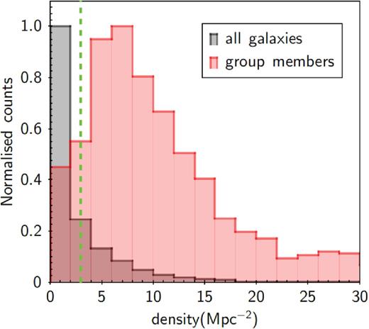
Density distribution around each galaxy with spectroscopic redshift in AEGIS, COSMOS, ECDFS and CDFN (in black) and group member galaxies in four mentioned fields (in red). The green dashed line at ρ = 3 galaxies Mpc⁻² shows the threshold to separate group from field galaxies. 73  per cent of all field galaxies are found at densities below this limit and 90 per cent of all group member galaxies are above that.

Open in new tabDownload slide

Similarly to Ziparo et al. (2014), we define a third environmental class of galaxies identified by density values similar to the ones of group galaxy members but not associated with any X-ray-extended emission observed in the X-ray surveys considered in this work. These galaxies have density above the ρ = 3 galaxies Mpc⁻² threshold and do not lie in the sky region defined by detected X-ray-extended emissions. They likely belong to filaments, sheet-like structures or to groups at lower mass with respect to the mass limit imposed by the CDFS, CDFN, AEGIS and COSMOS X-ray detection limits. We define this class of objects as ‘filament-like’ galaxies. With this approach, we define a sample of 1246 ‘filament-like’ galaxies in low redshift bin and 2320 in high redshift bin. This additional class of objects will be used also to check whether the relative vicinity of galaxies can affect galaxy properties as suggested by Peng et al. (2010, 2012) or, instead, the membership to a massive halo is a key ingredient in the galaxy evolution.

2.3 Morphology

We link the location of galaxies in the SFR–stellar mass plane also to the galaxy morphology. The galaxy morphological information are taken from the Advanced Camera for Surveys General Catalog (ACS-GC), which is a photometric and morphological data base based on publicly available data obtained with the Advanced Camera for Surveys (ACS) instrument on board of the Hubble Space Telescope (Griffith et al. 2012). This catalogue contains ∼370 000 galaxies observed in the AEGIS, COSMOS, GEMS and GOODS surveys. Briefly, Griffith et al. (2012) use galfit to measure the structural parameters of each galaxy by modelling each source with a single Sérsic profile (Sersic, Garcia Lambas & Mosconi 1986, see Graham & Driver 2005 for the mathematical relationship) together with a model for the sky. By cross-matching our galaxy catalogues of EGS, COSMOS and the GOODS fields with the ACS-GC, we find morphology information for 80 per cent of our galaxy sample. We use the structural measurements based on the ACS F850LP imaging in GOODS-South, based on the ACS F775W imaging in GOODS-North and on the ACS F814W imaging in COSMOS and AEGIS.

3 RESULTS

3.1 The non-linearity and dispersion of the SF galaxy MS

Before studying the location of galaxies in the SFR–stellar mass plane as a function of the environment, it is necessary to define the galaxy MS in our two redshift bins and estimate its dispersion. In doing this, we try to avoid any selection bias by applying the following procedure. First, we investigate if the MS is a linear relation (i.e. with a slope of unity) or if there is some level of non-linearity (deviation from a slope of 1, and possible curvature) at the high stellar masses as suggested by Whitaker et al. (2012, 2014). As a starting point, we look at the distribution of SFR of the IR-detected galaxies in the photometric redshift sample to avoid any selection bias which can be induced by spectroscopic selection function. Of course z_phot is replaced by the spectroscopic redshift whenever this is available. Figs 2 and 3 show SFR_IR distribution in different stellar mass bins for low- and high-redshift samples, respectively. The Gaussian curves are fitted to the right-hand side of the peaks of the distributions and their mirrors in the left-hand sides. The dispersions of the Gaussians are about 0.27–0.3 dex, consistent with the values reported by many previous studies (Daddi et al. 2007; Elbaz et al. 2007; Peng et al. 2010). However, these figures demonstrate that a Gaussian is not a good fit to the MS at least above 10^10.4 M_⊙ where we are absolute complete in IR data.

Figure 2.

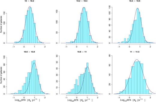
Distribution of SFR of all IR-detected galaxies at 0.15 < z < 0.5 in different stellar mass bins.

Open in new tabDownload slide

Figure 3.

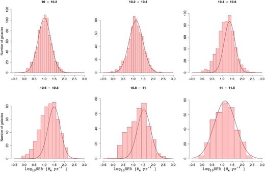
Distribution of SFR of all IR-detected galaxies at 0.5 < z < 1.1 in different stellar mass bins.

Open in new tabDownload slide

Figure 4.

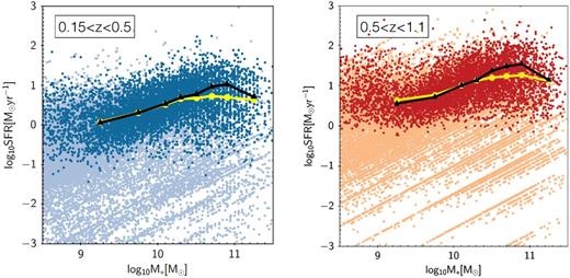
Left-hand panel: SFR versus M_* for galaxies in 0.15 < z < 0.5. The dark blue points show the IR-detected galaxies and the light blue points show galaxies with SFR_SED. The black connected triangles show the peak of distribution of SFR in different mass bins for IR-detected galaxies and the yellow connected circles show the mean of SFR for IR-detected galaxies. Right-hand panel: same as left-hand panel for galaxies in 0.5 < z < 1.1.

Open in new tabDownload slide

Figure 5.

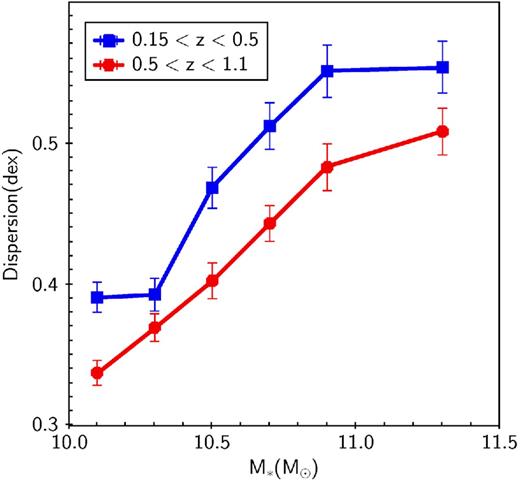
Dispersion around the MS location as a function of the galaxy stellar mass for high redshift bin (in red circles) and low redshift bin (in blue squares). Errors on the dispersion are calculated from bootstrapping.

Open in new tabDownload slide

Figure 6.

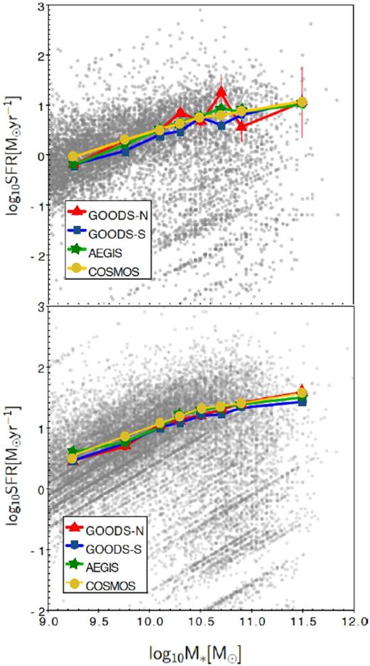
Upper panel: SFR versus M_* for galaxies in 0.15 < z < 0.5. The colourful connected circles show the mean of SFR for star-forming galaxies in different fields. Lower panel: same as left-hand panel for galaxies in 0.5 < z < 1.1.

Open in new tabDownload slide

In several works in the literature, the MS of star-forming galaxies is expressed through a linear relation with slope consistent to 1 (Elbaz et al. 2007 for 0.8 < z < 1.2, Noeske et al. 2007 for 0.2 < z < 0.7 and Peng et al. 2010 for 0.02 < z < 0.085). Peng et al. (2010), in particular, show that the MS of blue star-forming galaxies selected from the SDSS spectroscopic catalogue is linear up to very high masses and its slope and dispersion is independent from the environment. However, the selection of only blue galaxies as a way to isolate the bulk of the star-forming galaxies might affect their results. Indeed, Weinmann et al. (2006) show that 20 per cent of the galaxies hosted by massive haloes such as groups and clusters show red colours but a level of SF activity similar to the blue active galaxy population. In addition, Brinchmann et al. (2004) show that, when all galaxies are considered, the MS of the local Universe is well identified at stellar masses below 10^10–10.5 M_⊙ but it breaks down at higher masses. More recently, Whitaker et al. (2014) show that the deviation from a linear relation of the MS at high stellar masses is evident up to redshift ∼2. This would be consistent also with the relatively flat slope of the MS found by Rodighiero et al. (2010) up to z ∼ 2.5, obtained by stacking analysis in the Herschel PACS data.

3.2 The role of environment in shaping the MS

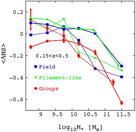
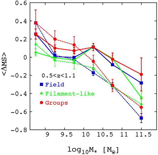
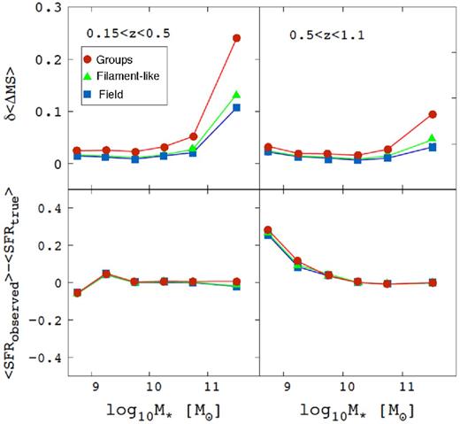
To investigate if the environment plays any role in shaping the MS, we analyse the deviation of the MS from the linear relation in the three environments defined in Section 2.2. This is done to check if the environment can be a cause either of the flattening of the MS or of the larger dispersion at high stellar masses. Fig. 7 shows the MS offset with respect to the reference linear relation (ΔMS) as a function of stellar masses for field galaxies (blue points), ‘filament-like’ galaxies (green points) and group galaxies (red points) in the low redshift bin (left-hand panel) and in the high redshift bin (right-hand panel). The analysis of these two plots leads to the following conclusions:

• the deviation of the MS from the linear relation at stellar masses above 10^10.4 M_⊙ exists in all environments;

• this deviation is in place already at z ∼ 1.1;

• at low redshift, group galaxies show a much more significant departure from the mean MS field at any stellar mass with respect to field and ‘filament-like’ galaxies;

• at higher redshifts, groups member galaxies do not deviate from the mean relation and their MS coincides with the MS of the other two environments;

• field (isolated) and ‘filament-like’ galaxies MS are perfectly consistent at any redshift.

Figure 7.

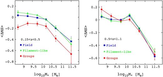
The MS offset for field, ‘filament-like and group star-forming galaxies as a function of stellar masses. <ΔMS> represents the mean of the residuals with respect to predicted MS in different stellar mass bins for low redshift bin (left-hand panel) and high redshift bin (right-hand panel). Errors are based on standard errors (see Appendix A).

Open in new tabDownload slide

The last evidence shows that the relative vicinity of galaxies as expressed by the density field is not playing an important role in affecting and/or regulating the galaxy SF activity. This, in addition to the blue galaxy selection, forms the likely explanation why Peng et al. (2010) did not observe any difference between the MS location of galaxies at different densities.

Fig. 7 indicates clearly that the evolution of the SF activity in galaxies does not depend only on the galaxy stellar mass through galaxy internal process (e.g. AGN feedback) but it must be regulated by also the environment in particular at the high stellar masses. Fig. 8 shows the SFR distributions of the IR-detected galaxies in group and field environments at low redshift. It illustrates that group galaxies are mostly populating the fading tail of the SFR distribution in Fig. 2. Our results confirm the first indication of Ziparo et al. (2013) that group galaxies evolve in a much faster way with respect to galaxies in lower mass haloes in terms of quenching of the SF activity. Thus, the membership to a massive haloes and the effect of all physical processes in place in such haloes are likely to be responsible for the decrease of the SF activity in groups since z ∼ 1. Fig. 7 also explains the increase of the dispersion of the MS in the low redshift bin, as a function of the stellar mass shown in Fig. 5. Indeed, the deviation of group galaxies towards a flatter and lower MS with respect to the mean relation has the effect of a broadening of the mean MS.

Figure 8.

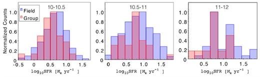
The distribution of SF of IR-detected star-forming galaxies for the field (in blue) and the group galaxies (in red) in different stellar mass bins at low redshift.

Open in new tabDownload slide

3.3 The role of morphology in the shape and dispersion of MS

To make a step further, we investigate also the relation of morphology, SFR and environment in the SFR–stellar mass plane. This is done to understand if the quenching of the SFR in group galaxies is also associated with a morphological transformation. For this purpose, we study the location of the MS in different environments as a function of the morphology. We identify three classes of galaxies on the basis of the Sérsic index value (see Section 2.3): galaxies with Sérsic index below 1.5 are classified as disc-dominated, galaxies with values between 1.5 and 2.5 are classified as intermediate-type galaxies, and galaxies with Sérsic index above 2.5 are classified as bulge-dominated systems. Consistently with Wuyts et al. (2011), above 10¹⁰ M_⊙ galaxies are located across the MS as a function of the morphology. Disc-dominated galaxies populate the upper envelope and intermediate-type galaxies are just above the bulge-dominated systems located on the lower envelope of the MS in any redshift bin, as shown in Fig. 9. We point out that the flattening of the MS above the stellar mass threshold of 10^10.4 M_⊙ seems to be more evident for the bulge-dominated galaxies, while disc-dominated galaxies tend to show a more linear relation. This result would indicate that the flattening of the MS is more related to the morphological evolution of galaxies rather than the effect of the environment. In addition, the displacement of bulge-dominated galaxies at lower SFR in the high stellar mass regime could contribute to the larger scatter of the relation in the high stellar mass regime.

Figure 9.

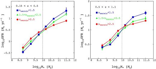
The mean of dependence of log SFR on stellar masses of MS galaxies in three different Sérsic index ranges for the low (left-hand panel) and high redshift bin (right-hand panel).

Open in new tabDownload slide

We further study the location of the MS as a function of morphology and environment in Figs 10 and 11. These figures show the mean ΔMS per stellar mass bin of each class of galaxies with respect to the reference MS linear relation in the low and high redshift bins. In order to have enough statistics, we divide galaxies only in two morphological classes: disc-dominated galaxies (Sérsic index < 2) and bulge-dominated ones (Sérsic index > 2). Fig. 11 shows that, at high redshifts, in all environments, disc-dominated and bulge-dominated galaxies are confirmed to occupy the upper and the lower envelope of the MS, respectively. At low redshift, in the group regime, instead, at high stellar masses also the disc-dominated systems are located on the lower envelope of the relation as the bulge-dominated counterpart (Fig. 10). This illustrates that the suppression of SF in disc-dominated galaxies causes the deviation of the group star-forming galaxies from other environments towards lower SFR. This also indicates that a quenching of the SFR is happening before any morphological transformation in the group regime. As a further step, we check the fraction of star-forming-bulge-dominated galaxies to the total star-forming galaxies as a function of environment. To investigate the differences among the different environmental classes, we calculate the fraction in several mass bins. This is done to take into account the stellar mass dependence of the flattening of the MS and the differential role of the environment at different mass scales. Fig. 12 shows that the Sérsic index distribution for MS galaxies is quite similar in all environmental classes both at low (left-hand panel) and high (right-hand panel) redshift. Fig. 12 in addition to Fig. 10 suggest that the SF quenching observed in group galaxies in Fig. 7 is not associated with systematic morphological transformation. We stress that this is not at odds with the well-known ‘morphology–density’ relation. Indeed, this more general relation reflects the differential morphological-type distribution of the entire galaxy population without distinction between galaxies on and off the MS. In this particular analysis, we consider only MS galaxies to show that the departure of group galaxies from the MS is not related to a morphological transformation. Instead, Fig. 12 shows clearly a much stronger dependence of the Sérsic index distribution on the stellar mass at low and high redshift. While below 10^10.4 M_⊙, MS galaxies tend to be late type, above this threshold the morphological-type distribution is clearly dominated by intermediate type (1.5 < Sérsic index < 2.5) and early-type (Sérsic index > 2.5) galaxies. This fact in addition to the shallower slope for bulge-dominated MS galaxies explain why we measure a shallower slope for MS galaxies.

Figure 10.

The MS offset for field, ‘filament-like’ and group star-forming galaxies as a function of stellar masses in the low redshift bin for disc-dominated (n_sersic < 2 with solid lines) and bulge-dominated galaxies (n_sersic > 2 with dashed lines).

Open in new tabDownload slide

Figure 11.

The MS offset for field, ‘filament-like’ and group star-forming galaxies as a function of stellar masses in the high redshift bin for disc-dominated (n_sersic < 2 with solid lines) and bulge-dominated galaxies (n_sersic > 2 with dashed lines).

Open in new tabDownload slide

Figure 12.

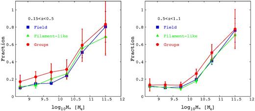
Left-hand panel: fraction of MS galaxies with Sérsic index n > 2 to total MS galaxies as a function of the stellar mass in the low redshift bin in three environmental classes: groups (red points and line), ‘filament-like’ galaxies (green points and line) and field galaxies (black points and line). Right-hand panel: same as the left-hand panel for the high redshift bin.

Open in new tabDownload slide

4 DISCUSSION

In this paper, we present the properties of the SF MS and its connection to morphology and host environment of galaxies since z ∼ 1.1. Both the dispersion and the slope of the MS unravel fundamental information about the efficiency and stochasticity of the processes which regulate the SF. We see that the distribution of SFR for IR-detected galaxies is not a Gaussian distribution till 10¹¹ M_⊙. The distribution of SFR at high stellar masses is skewed towards lower SFR at low and high redshift. However, the peak of distribution is consistent with a linear relation as found in previous studies. Above 10¹¹ M_⊙, either there is no MS at all or there is a shift of the peak towards low SFR. The existence of a long tail of the SFR distribution towards low SFR leads to an increase of the dispersion of the MS at higher masses. Below 10^10.4–10.6 M_⊙ the dispersion is 0.3–0.4 dex, consistent with the value reported by many of previous studies (Daddi et al. 2007; Elbaz et al. 2007; Peng et al. 2010). Above this mass limit it increases up to 0.5–0.6 dex.

In agreement with our results Lee et al. (2015), using far-IR photometry from Herschel-PACS, SPIRE and Spitzer-MIPS 24 μm, find that the relationship between median SFR and M_* follows a power law at low stellar masses, and flattens to nearly constant SFR at high stellar masses at z < 1.3. Whitaker et al. (2014) also find that the slope of the MS is dependent on stellar mass. They find that MS has roughly constant slope of unity for M_* < 10^10.2 M_⊙ and a shallower slope for the high-mass end spanning the redshift range 0.5 < z < 2.5. In addition, Huang et al. (2012) using a sample of galaxies in the local universe from SDSS suggest a transition mass of 10^9.5 M_⊙ below which SF scales differently with total stellar mass (also found by Salim et al. 2007) with a steeper slope. Rodighiero et al. (2010) also find a rather flat MS at any redshift on the basis of Herschel PACS data. Leja et al. (2015) find, by exploring the connection between the observed MS and stellar mass function, that the shallow slope for the MS cannot be hold for the low masses.

According to Figs 9 and 12, bulge-dominated galaxies are the main deriver of the flattening of the MS since galaxies with lower Sérsic index(disc-dominated galaxies with n_Sersic < 1.5) have a steeper MS. Furthermore, the presence of such bulge-dominated galaxies in the lower envelope of the MS explains the increase in the width of MS for the high-mass end. Wuyts et al. (2011) find that across cosmic time, the typical Sérsic index of galaxies is optimally described as a function of their position relative to the MS at the epoch of their observation. The correspondence between mass, SFR, and structure, as quantified by the Sérsic index, is equivalent to the Hubble sequence. Based on a quite similar galaxy sample (using SDSS for nearby universe and COSMOS, UDS and GOODS fields for high-redshift samples), Wuyts et al. (2011) see that such a sequence already existed at z ∼ 2; bulge-dominated morphologies go hand in hand with a more quiescent nature. In addition, they observe that late-type galaxies (Sérsic index < 1.5) follow a linear SFR–mass relation. Indeed, we also observe that late-type galaxies follow a linear relation (see Fig. 9). Nevertheless, they do not represent the bulk of the MS galaxy population above 10^10.4 M_⊙, but only the upper envelope. This means that, while a clear morphological sequence with a linear slope and, thus, a strong stellar mass dependence, is visible in the SFR–stellar mass plane at any mass as shown by Wuyts et al. (2011), the MS of star-forming galaxies at high masses is much more poorly defined and it shows a much weaker dependence on the stellar mass. This MS is consistent with a linear relation only in the low stellar mass range where it is dominated by late-type galaxies. At high masses, late-type galaxies are no longer the bulk of the MS population. There, morphological sequence and star-forming galaxy sequence are no longer overlapping. In agreement with our results, Whitaker et al. (2012) also find by selecting blue galaxies, the slope of unity for MS will be reached consistent with Peng et al. (2010). Consistently with our results, Lang et al. (2014), using a mass-selected galaxies, above 10¹⁰ M_⊙, observe a rising trends of the median Sérsic index and bulge to total ratio (B/T) of star-forming galaxies with increasing stellar mass at z ∼ 1 and 2. Moreover, using a sample of SDSS galaxies, Abramson et al. 2014 find that renormalizing SFR by disc stellar mass reduces the |$M_{{\ast }}\text{-}$|dependence of SF efficiency by ∼0.25 dex dex⁻¹, reducing the slope by 0.25. They also suggest that the non-linearity of MS may simply reflect the well-known increase in bulge mass-fractions with stellar mass.

Our study of the MS in different environments demonstrates that the environment does not seems to be the cause of the flattening of MS at high stellar masses, since the MS shows the same type of flattening in all environments. Moreover, at high redshift, group galaxies are perfectly on sequence as galaxies in the other environments. We only observe a significant decline of SFR of star-forming group galaxies at low redshift. This is consistent with previous studies in the literature. Indeed, the environmental trends at fixed stellar mass seem to weaken at higher redshift (e.g. Poggianti et al. 2008; Tasca et al. 2009; Cucciati et al. 2010; Iovino et al. 2010; Kovač et al. 2010; Ziparo et al. 2014). More recently, Popesso et al. (2015a) by the analysis of the IR luminosity function in groups find at z ∼ 1, Luminous IR galaxies (LIRGs) and Ultra-Luminous Infrared galaxies (ULIRGs) have contributions about 70 and 100 per cent, respectively, to group galaxies while these contributions reach to less than 10 per cent for the nearby groups. Consistently with these results, Popesso et al. (2015b), show that the cosmic SF history declines faster in group-sized haloes. Indeed, we also observe a faster evolution in the SF activity of star-forming galaxies inhabiting in group environments. We find that this faster evolution is independent of stellar mass. Indeed, this faster evolution and decline of SF activity in group environments acts in terms of increasing the scatter around the MS. In Fig. 5 also there is evidences for our claim as we measure a larger width for the MS in low-z sample. In addition, numerous previous studies of low-redshift galaxies in the literature find that colour and SFR are more strongly correlated with the environment than morphology (e.g. Kauffmann et al. 2004; Blanton et al. 2005; Christlein & Zabludoff 2005; van den Bosch et al. 2008; Weinmann et al. 2009). The implication of these studies is that the well-known correlation between morphology and environment is secondary to the correlation between environment and SFR. This is consistent with our findings. Indeed, we observe that among MS galaxies the distribution of the morphological type does not depend on the environment. However, at the same time group galaxies tend to be more quenched with respect to field and filament-like galaxies. Our results imply that in mass quenching, there is a morphological transformation (bulge growth) preceding quenching, but in environmental quenching the quenching happens before any morphological transition (if the latter happens at all).

Our results suggest that above a mass threshold (∼10^10.4–10^10.6 M_⊙), stellar mass, morphology and environment act together in driving the evolution of the SF activity towards lower level. The presence of a massive bulge could be responsible of the so-called morphological quenching suggested by Martig et al. (2009). In this model, the presence of a dominant bulge stabilizes the gaseous disc against gravitational instabilities needed for SF. This would be consistent with the results obtained by Whitaker et al. (2015), using a photometric mass-complete sample of galaxies at 0.5 < z < 2.5. They find that the scatter of the MS is related in part to galaxy structure. According to their results, they suggest a rapid build-up of bulges in massive galaxies at z ∼ 2. At z < 1, the presence of older bulges within star-forming galaxies decreasing the slope and contributing significantly to the scatter of the MS.

Another possibility may be the growth of the central supermassive BH which is the primary quenching agent for massive galaxies and is tightly coupled with the growth of bulges through both merging and disc instabilities (see SAM of Somerville et al. 2008). We note that this process is in place beyond z ∼ 1.1 (Lang et al. 2014; Whitaker et al. 2014). The environmental effects appear, instead, at lower redshifts. Our results suggest that the environmental process, responsible for the suppression of SF activity, should be a slow one as also suggested by Popesso et al. (2015b) and in agreement with Wetzel et al. (2013), De Lucia et al. (2012), Wheeler et al. (2014) and Simha et al. (2009).

The authors acknowledge Alvio Renzini and Michael L. Balogh for their useful comments and discussion on the early draft.

PACS has been developed by a consortium of institutes led by MPE (Germany) and including UVIE (Austria); KUL, CSL, IMEC (Belgium); CEA, OAMP (France); MPIA (Germany); IFSI, OAP/AOT, OAA/CAISMI, LENS, SISSA (Italy); IAC (Spain). This development has been supported by the funding agencies BMVIT (Austria), ESA-PRODEX (Belgium), CEA/CNES (France), DLR (Germany), ASI (Italy) and CICYT/MCYT (Spain).

This research has made use of NASA's Astrophysics Data System, of NED, which is operated by JPL/Caltech, under contract with NASA, and of SDSS, which has been funded by the Sloan Foundation, NSF, the US Department of Energy, NASA, the Japanese Monbukagakusho, the Max Planck Society, and the Higher Education Funding Council of England. The SDSS is managed by the participating institutions (www.sdss.org/collaboration/credits.html).

We gratefully acknowledge the contributions of the entire COSMOS collaboration consisting of more than 100 scientists. More information about the COSMOS survey is available at http://www.astro.caltech.edu/cosmos. This project has been supported by the DLR grant 50OR1013 to MPE.

REFERENCES

APPENDIX A: ERROR ANALYSIS

In order to estimate the errors in our analysis, we use the mock catalogue of Kitzbichler & White (2007). Using the available photometric bands (RJ), we simulate the spectroscopic selection function of the surveys used in this work by extracting randomly in each magnitude bin a percentage of galaxies consistent with the percentage of systems with spectroscopic redshift in the same magnitude bin observed in each of our surveys. We do this separately for each survey, since each field shows a different spectroscopic selection function (see fig. 5 in E14). We use this analysis to check for biases due to the spectroscopic selection function and to estimate the error due to the low number statistics. We create randomly 5000 ‘incomplete’ catalogues in this way in the low and high redshift bins. The dispersion around the difference between MS obtained from original complete catalogue (MS_complete) and the one from our simulation (MS_incomplete) for each environment provides the error on the ΔMS for that environment. The upper panels of Fig. A1 shows the error in different stellar mass bins for different environments in our two redshift bins. In order to see if our analysis are biased, we also look at the deviation of the MS_incomplete from MS_complete. The lower panels of Fig. A1 show that in high stellar masses (above 10^9.5), there is no bias due to high spectroscopic completeness. However, there is a bias at lower stellar masses which are not affecting our results. As the errors obtained in this way is lower than the standard errors, we keep the standard errors as the errors on ΔMS.

Figure A1.

Upper panels: dispersion around the MS_complete-MS_incomplete for simulated group galaxies (in red), filament-like galaxies (in green) and field galaxies (in blue) as a function of stellar mass. Lower panels: deviation of the simulated MS galaxies in different environment form the complete original mock catalogue as a function of stellar mass.

Open in new tabDownload slide

APPENDIX B: WAVELENGTH DEPENDENCE OF MORPHOLOGICAL MEASUREMENTS

Fig. B1 compares measurements of Sérsic index carried out on the WFC3 F215W mosaic and on the ACS F850LP and ACS F814W mosaics in GOODS-S and COSMOS, respectively. Median offsets are limited to the few per cent level for both low-z and high-z sample (2 and 8 per cent, respectively) and the dispersion around the one to one relation is about 18 per cent for low-z sample and 30 per cent for the high-z one.

Figure B1.

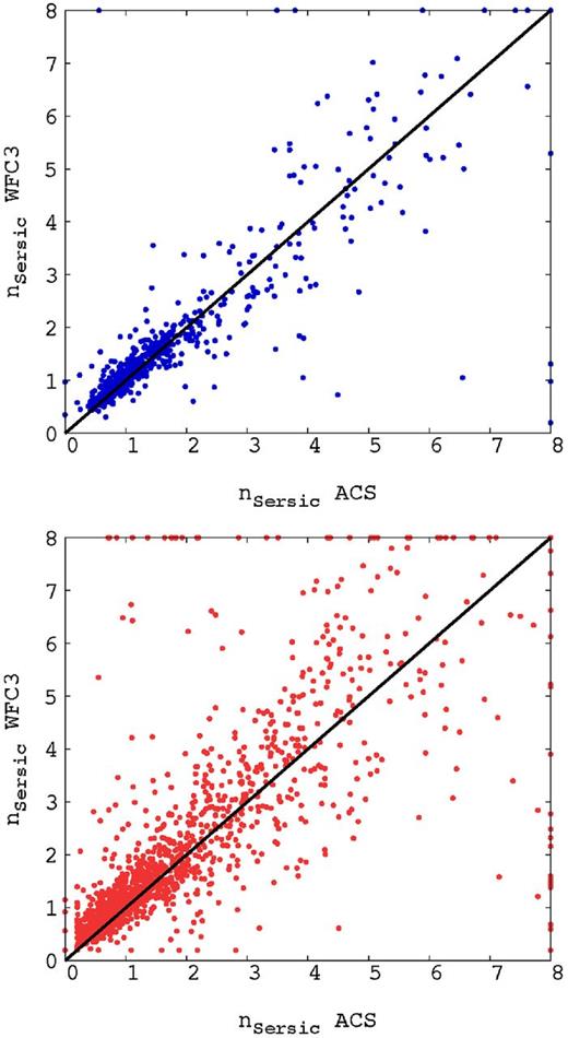
The Sérsic index measured on WFC3 F125W band versus ACS F850LP and ACS F814W bands in GOODS-S and COSMOS, respectively. The upper panel corresponds to the low-z sample and the lower panel shows the high-z one.

Open in new tabDownload slide