


Abstract
We introduce the BlueTides simulation and report initial results for the luminosity functions of the first galaxies and active galactic nuclei (AGN), and their contribution to reionization. BlueTides was run on the BlueWaters cluster at National Center for Super-computing Applications from z = 99 to 8.0 and includes 2 × 70403 particles in a 400 h−1 Mpc per side box, making it the largest hydrodynamic simulation ever performed at high redshift. BlueTides includes a pressure–entropy formulation of smoothed particle hydrodynamics, gas cooling, star formation (including molecular hydrogen), black hole growth and models for stellar and AGN feedback processes, and a fluctuating ultraviolet background from a patchy reionization model. The predicted star formation rate density is a good match to current observational data at z ∼ 8–10. We find good agreement between observations and the predicted galaxy luminosity function in the currently observable range −18 ≤ MUV ≤ −22.5 with some dust extinction required to match the abundance of brighter objects. The predicted number counts for galaxies fainter than current observational limits are consistent with extrapolating the faint-end slope of the luminosity function with a power-law index α ∼ −1.8 at z ∼ 8 and redshift dependence of α ∼ (1 + z)−0.4. The AGN population has a luminosity function well fit by a power law with a slope α ∼ −2.4 that compares favourably with the deepest CANDELS GOODS fields. We investigate how these luminosity functions affect the progress of reionization, and find that a high Lyman α escape fraction (fesc ∼ 0.5) is required if galaxies dominate the ionizing photon budget during reionization. Smaller galaxy escape fractions imply a large contribution from faint AGN (down to MUV = −12) which results in a rapid reionization, disfavoured by current observations.
1 INTRODUCTION
Recent deep observations using the Hubble Space Telescope have detected a plethora of objects at ever higher redshift (Bouwens et al. 2015a; McLeod et al. 2015; Oesch et al. 2015) and measured the galaxy ultraviolet (UV) luminosity function at z ≤ 10. At these redshifts, microwave background measurements suggest that a substantial fraction of the Universe is still neutral (Hinshaw et al. 2013), and these observations may therefore probe the epoch of reionization. In the near future, next-generation space missions such as JWST (Gardner et al. 2006) and WFIRST (Spergel et al. 2013) will increase the number of available samples by several orders of magnitude. These are expected to detect the sources which produce the ionizing photons that drive reionization.
The formation of these objects is driven by non-linear gravitational collapse and so understanding them requires cosmological hydrodynamic simulations. The presence of an ionizing background may affect galaxy formation (Madau, Pozzetti & Dickinson 1998). To model the processes governing reionization it is desirable to simultaneously include scales of a few hundred Mpc, the characteristic size of ionization bubbles, and, to resolve the formation of galactic haloes, scales of a few kpc.
We present results from BlueTides, the largest cosmological hydrodynamic simulation yet performed, enclosing a box 400 h−1Mpc on a side, with a smoothing length of 1.5 h−1Kpc, and including 2 × 70403 particles – a total of 0.7 trillion particles. Our high resolution allows us to study the formation of disc galaxies (Feng et al. 2015a), while the large volume allows study of the progress of reionization.
We include a number of physically relevant processes, including star formation incorporating the effects of molecular hydrogen formation (Krumholz & Gnedin 2011), energetic feedback from supernovae (Okamoto et al. 2010), and feedback from supermassive black holes (Di Matteo, Springel & Hernquist 2005). We include for the first time in a simulation of this size a model for patchy reionization which varies the optical depth based on local density (Battaglia et al. 2013).
Several large volume simulations have recently been performed. In particular, MassiveBlack I was the largest volume hydrodynamic simulation Di Matteo et al. (2012) to study reionization at z > 4.75. MassiveBlack II simulated a 100 h−1Mpc volume at substantially improved resolution to z = 0 (Khandai et al. 2015). Illustris included a volume and resolution comparable to MassiveBlack II, but with improved prescriptions for the effect of energy injection from supernovae (Okamoto et al. 2010). The Eagle simulation is similar in size to MassiveBlack II and Illustris, but with a different approach to sub-grid modelling which allows improved agreement with observations by weakening requirements for numerical convergence with resolution (Schaye et al. 2015). Concurrently, dark matter-only simulations have continued to increase in size, reaching loads of trillions of particles (Habib et al. 2016).
BlueTides is based on the simulation code used in MassiveBlack I and II, p-gadget3 (Springel 2005; Di Matteo et al. 2012; Khandai et al. 2015). The simulation encloses a volume comparable to MassiveBlack I, has a resolution comparable to MassiveBlack II, and includes a stellar feedback model similar to that of Illustris. Our particle load is 10 times larger than that of MassiveBlack I, which was previously the largest hydrodynamic simulation.
In Section 2 we present our methods, explaining briefly the computational techniques necessary to perform a simulation of this magnitude. In Sections 3 and 4 we examine the basic statistics of objects within the simulation. We show the galaxy and active galactic nuclei (AGN) UV luminosity functions and star formation rates (SFRs), and we present fits to these functions for easy comparison with future observations. In Section 5 we compute the sources of ionizing photons within our model and use them to examine features of reionization. Finally we conclude in Section 6.
2 BLUETIDES: SOFTWARE AND SUB-GRID PHYSICS
The BlueTides simulation was performed on the BlueWaters cluster at the National Center for Super-computing Applications (NCSA). We operated the production run on a total of 648 000 Cray XE compute core of BlueWaters. This is the largest cosmological hydrodynamic simulation to date, containing a simulation volume roughly 300 times larger than the largest observational survey at redshift 8–10 (Trenti et al. 2011). This extraordinary size allows us to easily compare our results to current and future observations, and obtain a representative sample of the first galaxies which may have driven reionization. A visual overview of the simulation is shown in Fig. 1.

Overview of the BlueTides simulation. Left inset: a field of view from the BlueTides simulation at z = 8 with the same total area as the BoRG survey (Trenti et al. 2011). Right inset: the field of view of the entire BlueTides simulation at z = 8. Background: galaxies in BlueTides. Even rows: top, front, and side views of the gas component of FoF haloes. Odd rows: top, front, and side views of the SFR surface density of FoF haloes.
Haloes in BlueTides are identified using a Friends-of-Friends (FoF) algorithm with a linking length of 0.2 times the mean particle separation (Davis et al. 1985). We have not performed sub-halo or spherical overdensity finder algorithms on BlueTides due to limits on the scalability of current implementations. We will however investigate the mass function with spherical overdensity finders in a follow-up work.
2.1 Computing: improved performance at peta-scale
At the particle numbers reached by our simulation, any unnecessary communication overhead can easily become a significant scalability bottleneck. In order to allow the simulation to fully utilize the available computational power, we implemented several improvements to the speed and scalability of the code. Here we briefly list the substance of the most important changes, deferring a fuller description to Feng (2015, in preparation).
First, we substantially improved the scalability of the threaded tree implementation, which computes short-range particle interactions. This includes the gravitational force on small scales, hydrodynamic force, and the various feedback processes. Our improved routine scales to >30 threads and at 8 threads is twice as fast as the previous implementation in p-gadget3. Scalability improvements were achieved by eliminating OpenMP critical sections in favour of per-particle posix spin-locks, essentially making the thread execution wait-free at high probability.
Secondly, we replaced the default particle mesh gravity solver (used to compute long-range gravitational forces) based on FFTW with a gravity solver based on a 2D tile FFT library, pfft (Pippig 2013). This allows a more efficient decomposition of particles to different processors, significantly improving the load and communication balance. To further simplify the book keeping and reduce memory overhead, we switched to using Fourier-space finite differencing of gravity forces, as used by the N-body gravity solver HACC (Habib et al. 2016). We also reduced the communication load by applying a sparse matrix compression of the local particle mesh. In concert these changes removed the Particle Mesh (PM) step as a scalability bottleneck.
Thirdly, at the high redshift covered by BlueTides, only a small fraction of the particles are in collapsed haloes. Thus, to ease analysis, we produce two digest data sets on the fly in addition to the full simulation snapshots: (1) Particles-In-Group (PIG) files, which contain the attributes of all particles in the overdense regions detected by the FoF groups; (2) Sub-sample files, containing a fair sub-sample of 1/1024 of the dark matter and gas particles, and a full set of star and black hole particles.
Fourthly, we implemented a histogram-based sorting routine to replace the merge sort routine originally present in p-gadget3. Histogram-based sorting routines have been shown to perform substantially better at scale (Solomonik & Kale 2010), a result confirmed by our experience in BlueTides (Feng et al. 2015b). Particles must be sorted when constructing the FoF group catalogues, and our new sort routine sped up FoF catalogue generation times by a factor of 10. The source code of this sorting routine, mp-sort, is available from http://github.com/rainwoodman/MP-sort to facilitate independent reuse.
Finally, we implemented a new snapshot format (bigfile) that supports transparent file-level striping and substantially eases post-production data analysis compared to multiple plain Hierarchical Data Format Version 5 (HDF5) files. Until recently, file-level striping [bypassing Message Passing Interface – Input/Output (MPI-IO)] has been the only way to achieve the full IO capability of Lustre file system for problems at our scale. We release the library for accessing the BlueTides simulation at http://github.com/rainwoodman/bigfile, together with python language bindings for post-simulation data analysis.
2.2 Physics: hydrodynamics and sub-grid modelling
BlueTides uses the hydrodynamics implementation described in Feng et al. (2014). We adopt the pressure-entropy SPH (pSPH) to solve the Euler equations (Read, Hayfield & Agertz 2010; Hopkins 2013). The density estimator uses a quintic density kernel to reduce noise in SPH density and gradient estimation (Price 2012).
Table 1 lists the basic parameters of the simulation. Initial conditions are generated at z = 99 using an initial power spectrum from CAMB (Lewis & Bridle 2002). Star formation is implemented based on the multiphase star formation model in Springel & Hernquist (2003), and incorporating several effects following Vogelsberger et al. (2013). Gas is allowed to cool both radiatively following Katz, Weinberg & Hernquist (1996) and via metal cooling. We approximate the metal cooling rate by scaling a solar metallicity template according to the metallicity of gas particles, following Vogelsberger et al. (2014). We model the formation of molecular hydrogen, and its effect on star formation at low metallicities, according to the prescription by Krumholz & Gnedin (2011). We self-consistently estimate the fraction of molecular hydrogen gas from the baryon column density, which in turn couples the density gradient into the SFR.
Parameters of the BlueTides simulation.
| Name | Value | Notes |
|---|---|---|
| |$\Omega _\Lambda$| | 0.7186 | |
| ΩMatter | 0.2814 | Baryons + Dark matter. |
| ΩBaryon | 0.0464 | |
| h | 0.697 | Hubble parameter in units of 100 km s−1 Mpc−1. |
| σ8 | 0.820 | |
| ns | 0.971 | |
| LBox | 400 h−1Mpc | Length of one side of the simulation box. |
| NParticle | 2 × 70403 | Total number of gas and dark matter particles in the initial conditions. |
| MDM | 1.2 × 10⁷ h−1M⊙ | Mass of a dark matter particle. |
| MGAS | 2.36 × 10⁶ h−1M⊙ | Mass of a gas particle in the initial conditions. |
| ηh | 1.0 | SPH smoothing length in units of the local particle separationa. |
| εgrav | 1.5 h−1Kpc | Gravitational softening length. |
| NGeneration | 4 | Mass of a star particle as a fraction of the initial mass of a gas particle. |
| egyw/egy0 | 1.0 | Fraction of supernova energy deposited as feedback. |
| κw | 3.7 | Wind speed as a factor of the local dark matter velocity dispersion. |
| ESNII, 51 | 1.0 | Supernova energy in units of 1051 erg s−1. |
| |$M^{(0)}_\mathrm{BH}$| | 5 × 10⁵ h−1M⊙ | Seed mass of black holes. |
| |$M^{(0)}_\mathrm{HALO}$| | 5 × 10¹² h−1M⊙ | Minimum halo mass considered in black hole seeding. |
| ηBH | 0.05 | Black hole feedback efficiency. |
Note.aA value of 1.0 translates to 113 neighbour particles with the quintic kernel used in BlueTides.
We model feedback from AGN in the same way as in the MassiveBlack I and II simulations, using the supermassive black hole model developed in Di Matteo et al. (2005). Supermassive black holes are seeded with an initial mass of 5 × 10⁵ h−1M⊙ in haloes more massive than 5 × 10¹⁰ h−1M⊙, while their feedback energy is deposited in a sphere of twice the radius of the SPH smoothing kernel of the black hole. Black hole seeding masses from 100 to 106 M⊙ have been suggested depending on the formation scenario (Volonteri 2010). Our choice of seeding mass is closer to that expected from direct collapse scenarios (e.g. Latif et al. 2013; Schleicher et al. 2013; Ferrara et al. 2014). We note however that our seeding scheme makes no direct assumption of the black hole formation mechanism. The seeding scheme effectively assumes that AGN feedback are neglected in haloes less massive than 5 × 10 M⊙ h−1.
The large volume of BlueTides allowed us to include some of the effects of ‘patchy‘reionization, where the amplitude of the UV background is spatially variable. We model patchy reionization using a semi-analytic method based on hydrodynamic simulations performed with radiative transfer (for more details see Battaglia et al. 2013). This method uses an evolved density field calculated from the initial conditions using second-order Lagrangian perturbation theory to predict the redshift at which a given spatial region will reionize. In our fiducial reionization model, we set the mean reionization redshift at z ∼ 10 based on the measurement of the optical depth, τ, from the WMAP 9 year data release (Hinshaw et al. 2013). In regions that have been reionized, we assume the UV background estimated by Faucher-Giguère et al. (2009). The global neutral fraction in BlueTides evolves smoothly as a function of redshift, as seen in Fig. 2.
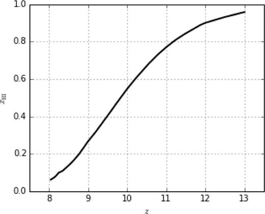
Global neutral hydrogen fraction as a function of redshift in BlueTides.
3 STAR FORMATION RATE
Fig. 3 shows the global SFR in BlueTides, together with observational constraints and several other simulations. We show the total star formation density in the whole volume (dotted lines) and the total SFR for haloes with SFR > 0.7 M⊙ yr−1 (solid line). The latter is directly comparable with current observations and corresponds to the current observational limit of MUV = −18. The SFR density in BlueTides smoothly increases with decreasing redshift.

The star formation rate density (SFRD) in the BlueTides simulation. Solid blue: SFRD of haloes with SFR greater than 0.7 M⊙ yr−1 from BlueTides. Dashed black: SFRD of equivalent haloes from Illustris (Genel et al. 2014; Vogelsberger et al. 2014). Solid black: SFRD of equivalent haloes from MassiveBlack II (Khandai et al. 2015). Dotted blue: SFRD of all haloes from BlueTides. Dotted black: SFRD of all haloes from MassvieBlack II. Squares: estimates from HUDF (Oesch et al. 2014), and HFF A2744 (Oesch et al. 2015). Diamonds: observational estimates from CLASH (Zheng et al. 2012; Coe et al. 2013; Bouwens et al. 2014a). Illustris, CLASH, and HUDF lines are reproduced from Oesch et al. (2015). Wide grey: global black hole accretion rate density in BlueTides, scaled by 103 (see text).
Several Hubble Ultra Deep Field surveys have given estimates on the star formation rate density (SFRD) due to haloes with MUV < −18. BlueTides haloes at the observational limit typically contain a few thousand particles, and are thus well resolved. The BlueTides predictions for the SFR are in good agreement with current observations, with the caveat that at these high redshifts observational uncertainty remains high.
Fig. 3 also compares the SFR density in BlueTides to that from two other recent (albeit smaller volume) simulations: Illustris (Genel et al. 2014; Vogelsberger et al. 2015), and MassiveBlack II (Khandai et al. 2015). Illustris uses similar prescriptions for sub-grid feedback, but a different solver for the Euler equations, while MassiveBlack II uses substantially different sub-grid modelling, which is less effective at suppressing star formation in faint objects. Neither of the other simulations includes patchy reionization. The SFRs for BlueTides and Illustris agree very well, while that for MassiveBlack II is a factor of a few larger. This suggests that the sub-grid feedback model dominates in controlling the SFR over both the choice of hydrodynamic method and the effect of reionization. It is however promising to see, given the differences in the simulations, that the differences are within at most a factor of a few in SFR density.
Fig. 3 also shows the evolution of the global black hole accretion rate density. The black hole accretion rate grows more rapidly than the global SFRD. This is likely due to an increase in the number density of black hole hosting haloes; in contrast, the black hole mass–stellar mass relation remains constant over time (MBH = 10−3Mstar).
In Fig. 4, we show the cumulative SFRD from galaxies of different halo mass. For comparison, we also calculated the cumulative SFR density of Illustris at three corresponding redshifts (z = 8, 9, 10). We see that the mass threshold for 50 per cent of star formation increases from ∼5 × 10⁹ h−1 M⊙ at z = 13 to ∼4 × 10¹⁰ h−1 M⊙ at z = 8. Thus the contribution of small haloes to the ionizing photon budget becomes increasingly important at higher redshift. The larger volume in BlueTides means that it includes haloes 10 times more massive than the most massive haloes in Illustris. These objects contribute less than 10 per cent of the total star formation density at z = 8, 9, and 10.

Cumulative SFRD in haloes. Coloured solid: cumulative SFRD in BlueTides. Gray dashed: cumulative SFRD in Illustris at z = 8, 9, 10, from the Illustris public data release (Nelson et al. 2015). Thick black: contour of 50 per cent cumulative SFRD. Thin black: contour of 10 per cent cumulative SFRD.
4 STELLAR AND AGN UV LUMINOSITY FUNCTIONS
In this section, we report the stellar AGN luminosity functions in BlueTides. We first describe our source detection method, using Source Extractor to validate the results of an FoF halo finder at these high redshifts (Section 4.1). We then describe the stellar UV luminosity function (Section 4.2.1), the dust attenuation model (Section 4.2.2), and the faint-end slope of the luminosity function (Section 4.2.3). We assemble the stellar luminosity function from BlueTides and compare to observations and other simulations (Section 4.2.4). Finally we report the AGN luminosity function(Section 4.3).
4.1 The identification of Galaxies in BlueTides: Source Extractor versus FoF
The FoF algorithm considers only the spatial positions of particles and can sometimes artificially group dynamically distinct objects into one halo. In this section we compare the luminosity function estimated from FoF catalogues to that which would be estimated by performing standard observational techniques and show that the difference is small.
Simulations and observations have long been defining objects in different ways. Even the sub-haloes in simulations do not directly translate to any imaging survey catalogues. In imaging surveys, objects are identified by selecting peaks in a two-dimensional image, and the total luminosity depends on an aperture radius. (we refer the readers to Stevens et al. 2014, and references therein) The canonical implementation of such an algorithm is Source Extractor (Bertin & Arnouts 1996). We use SEP, a reimplementation of Source Extractor into python (Barbary & contributors 2014).
We produce a mock 2D survey image by projecting the BlueTides simulation box along one axis. The SFRs of particles are distributed into pixels using a Gaussian kernel scaled by their SPH smoothing lengths with gaepsi (Feng et al. 2011). We do not attempt to model instrumental noise in the mock image. The final star formation surface density image has (2 × 10⁵)2 pixels, with a spatial resolution of 2 h−1Kpc per pixel (∼0.06 arcsec). This image is then divided into 100 non-overlapping equal-sized sub-volumes x–y plane. Each sub-volume has a volume of 40 × 40 × 400( h−1Mpc)3. This allows us to estimate the cosmic variance in e.g. the luminosity functions in fields comparable to those observed. We note that 400 h−1Mpc roughly corresponds to a redshift width of Δz ∼ 1 at z = 8.0, and hence each image chunk roughly corresponds to the full volume of the BoRG survey.

Detecting objects from the mock star formation intensity image. Background: the star formation intensity image of the full projection of BlueTides (400 h−1Mpc per side). We note that the image is strikingly uniform because of the thickness of the projection. Top left: the star formation intensity image of a single chunk, 40 h−1Mpc per side. Top right: all objects identified in a field of view with a 10 times zoom, 4 h−1Mpc per side. SEP objects are marked in red. Bottom right: a further zoomed-in view of the top-right panel, to show the identified objects more clearly.
As shown in Fig. 6, we find that the luminosity functions constructed from the FoF halo catalogue and the SEP imaging catalogue differ by less than 20 per cent. The main differences are that the SEP luminosity function includes fewer bright objects than the FoF luminosity function and more faint objects. Quantitatively, SEP is ∼80 per cent of FoF at MUV > −22 and ∼120 per cent of FoF at MUV < −18. These differences can be understood by noting that bright (massive) FoF haloes are often a cluster of smaller objects which SEP tends to identify as separate galaxies. The fixed aperture in SEP however tends to enhance the UV of smaller objects. These effects are smaller at these high redshifts, where large groups have not yet formed. Because these differences are small, we will use the FoF catalogue for the rest of this work.
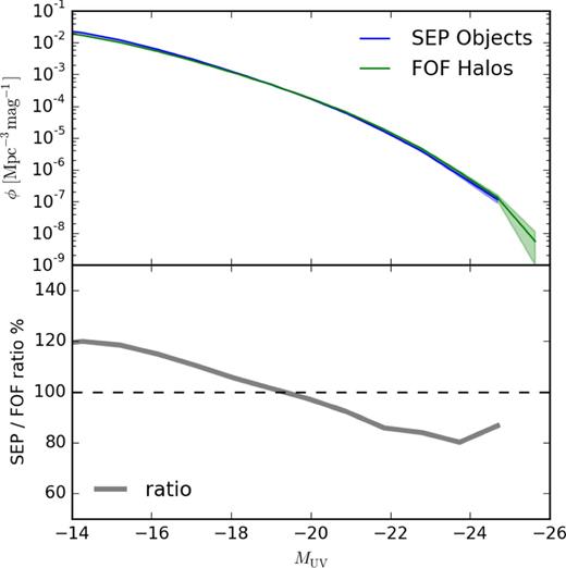
UV luminosity function of galaxies found with Source Extractor compared to that of FoF haloes at z = 8. Green: SEP catalogue. Blue: FoF catalogue. Solid grey: the ratio between SEP and FoF (axis on right).
4.2 Stellar luminosity functions
4.2.1 Intrinsic stellar luminosity functions

Evolution of the intrinsic UV luminosity function with redshift from z = 8 to 13 (colours online). Shaded regions show the 1σ sample variance of the mass functions. Dashed lines: best-fitting modified Schechter model. The vertical dashed line corresponds to the current observation limit of MUV ∼ −18.
This model differs from the usual Schechter model (see equation 5 below) only in that the coefficient that determines the rate of extinction of bright-end galaxies is changed from 0.4 to 0.1. The best-fitting values are shown in Table 2. The modified model agrees with the luminosity function at the 5 per cent level for the whole luminosity range of the simulation. Note that the change in the bright-end coefficient means that one should not directly compare these fit parameters with those obtained from a Schechter model. We also do not use this model to extrapolate the luminosity function (although with a minor 10 per cent difference in the photon budget, using it would not change our conclusions).
Best-fitting parameters of the modified Schechter model for the galaxy UV luminosity functions at z = 8–13. Parameters are fit using equation (3).
| z | αL | log ϕ⋆ | |$M_\mathrm{UV}^\star$| |
|---|---|---|---|
| 8 | −1.54 ± 0.01 | −4.04 ± 0.07 | −15.99 ± 0.09 |
| 9 | −1.59 ± 0.02 | −4.17 ± 0.14 | −15.44 ± 0.19 |
| 10 | −1.55 ± 0.04 | −3.66 ± 0.18 | −14.09 ± 0.28 |
| 11 | −1.51 ± 0.07 | −3.42 ± 0.21 | −13.03 ± 0.40 |
| 12 | −1.40 ± 0.07 | −3.42 ± 0.10 | −11.78 ± 0.37 |
| 13 | −1.32 ± 0.10 | −3.82 ± 0.08 | −10.98 ± 0.44 |
4.2.2 Dust extinction

Evolution of the UV luminosity function with dust extinction with redshift z = 8, 9, 10, 11, 12, 13. (colours online) Shaded regions show the 1σ uncertainty of the mass functions. Dashed lines: best-fitting modified Schechter model (see equation 5). The vertical dashed line corresponds to the current observational detection limit of MUV ∼ −18.
Best-fitting Schechter model parameters at z = 8–13 for galaxy stellar UV luminosity functions including dust extinction. Parameters are as described in equation (5).
| z | αL | log ϕ⋆ | |$M_\mathrm{UV}^\star$| |
|---|---|---|---|
| 8 | −1.84 ± 0.03 | −8.90 ± 0.21 | −20.95 ± 0.15 |
| 9 | −1.94 ± 0.03 | −9.74 ± 0.24 | −20.77 ± 0.17 |
| 10 | −2.01 ± 0.04 | −10.27 ± 0.33 | −20.39 ± 0.22 |
| 11 | −2.07 ± 0.05 | −10.77 ± 0.42 | −20.00 ± 0.27 |
| 12 | −2.12 ± 0.06 | −11.40 ± 0.50 | −19.65 ± 0.31 |
| 13 | −2.13 ± 0.06 | −11.71 ± 0.49 | −19.11 ± 0.30 |
4.2.3 Faint-end slope
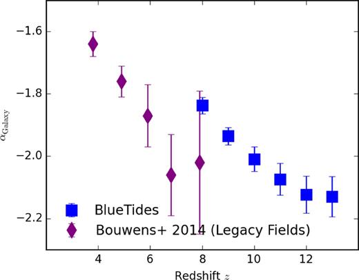
Evolution of the faint-end slope of the galaxy UV luminosity function. The purple diamonds are the observed slope from Hubble legacy surveys (Bouwens et al. 2015a). Blue circles show the slope from BlueTides.
The slope of the faint end of the UV luminosity is consistent with that inferred by Bouwens et al. (2015a) and its evolution with redshift implies moderate steepening, again consistent with an extrapolation of the observed slope evolution up to z = 12, which includes an evolution of M/L ratio ∝(1 + z)−1.5 due to the evolution of the Halo Mass Function.1 The faint end (MUV > −20) of the UV luminosity function in BlueTides is barely affected by the dust extinction model; thus the redshift-slope relation we give here is suitable for inputs of reionization calculations.
4.2.4 Comparison with observations and other models
Bouwens et al. (2015a) assembled and reanalyzed the UV luminosity function evolution from z = 10 to 4 based on all currently available legacy Hubble surveys. The total cumulative area is close to 1000 arcmin2, spread over a wide redshift range (see also Trenti et al. 2010; Ellis et al. 2013; Finkelstein et al. 2015). The most recent measurements at z = 10 were published in Oesch et al. (2014). Fig. 10 compares a compilation of these observational data to stellar UV luminosity functions from BlueTides. We show the BlueTides luminosity functions extracted from sub-fields with size roughly the area of the BoRG survey (Bouwens et al. 2015a), the legacy field with the currently largest area. As this is a smaller volume than the full simulation, we can use the differences between sub-volumes to estimate sample variance from current observations, which is shown by the shaded areas in Fig. 10. The intrinsic luminosity produces more bright galaxies than are observed, a discrepancy which is marginally significant compared to cosmic variance. After applying a dust extinction correction, this slight tension with observations largely disappears, suggesting that dust corrections are indeed significant for the brightest galaxies, even at these high redshifts. As we shall discuss in Section 4.3, another possibility is that the brightest sources host a significant AGN which may make their detection in the galaxy samples harder.

Comparing UV luminosity functions with observations. Solid blue: intrinsic UV luminosity function in BlueTides. The coloured bands shows the cosmic variance in a survey volume of the size of the BoRG survey (Bouwens et al. 2015a). Solid red: dust-reddened UV luminosity function in BlueTides. Dotted black: luminosity functions from the simulations of Jaacks et al. (2012). Note that they do not provide a simulated luminosity function at z = 10; also the largest volume at z = 9 was a 34 h−1Mpc box. Green wedges: intrinsic UV luminosity function from the Illustris public data release (Nelson et al. 2015). Black dashed line: intrinsic UV luminosity function from the MassiveBlack II public data (Khandai et al. 2015). Black squares: observed luminosity functions at z = 8 and 10 from Bouwens et al. (2015a). Black diamonds: observed luminosity function at z = 9 from McLure et al. (2013) and McLeod et al. (2015). Black circles: observed luminosity function from four bright galaxies at z ∼ 10 from Oesch et al. (2014).
We show comparisons with two other recent high-redshift simulations with a maximal volume of 100 h−1Mpc. Jaacks et al. (2012) performed several simulations at different resolutions to investigate the shape and slope of high-redshift galaxy UV luminosity function. The luminosity functions of Jaacks et al. (2012) have faint-end slopes which are steep compared to observations, producing substantially too many stars in small objects. This is likely due to their stellar feedback (Choi & Nagamine 2011) being insufficiently effective at suppressing star formation. We also show the corresponding UV luminosity function at z = 8, 9, 10 from the public data of Illustris (Nelson et al. 2015). Due to the larger volume in BlueTides, Illustris produces fewer bright objects and cannot be compared to BlueTides at the most massive end. However, at the faint end of the luminosity function (MUV < −20), BlueTides and Illustris agree at the 10 per cent level. This suggests that a stellar feedback model which very efficiently suppresses star formation in small haloes is the most important ingredient when matching the luminosity function at high redshift, just as at low redshift.
4.3 AGN luminosity function
Fig. 11 shows the UV luminosity function of AGN in BlueTides. The luminosity function is cut at MUV = −18.6, a limit dictated by the imposed seed mass of our black holes (Mseed = 5 × 10⁵ M⊙). The black hole luminosity function is only meaningful for objects that have at least doubled their mass since the black hole was seeded, thereby erasing the artificially imposed seed mass. For smaller black holes the AGN luminosity function is significantly suppressed due to the artificial absence of black holes in our numerical scheme. Most of these galaxies have a stellar mass of a few times 107 h−1M⊙, ∼100 times of the seed mass.
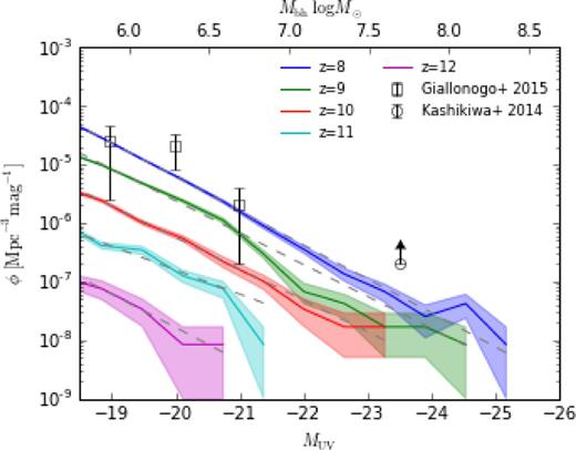
AGN UV luminosity function from BlueTides. The coloured bands show the 1σ sample variance estimated from 100 sub-volumes (see Section 2). We cut the luminosity function at the faint end at MUV = −18.6, corresponding to the seed mass of the black holes in BlueTides. Dashed lines: the best-fitting power-law model. Symbols: measurements at z = 5.75 by Giallongo et al. (2015) and Kashikawa et al. (2015).
The AGN luminosity function rises steadily at later times, mirroring the evolution in the stellar luminosity function. By z ≥ 13 our box contains a negligible number of AGN and it is thus impossible to reliably estimate the luminosity function.
Best-fitting power-law parameters at z = 8–12 of the AGN UV luminosity function. The fitting model is described by equation (9).
| z | αL | log ϕ⋆ |
|---|---|---|
| 8 | −2.45 ± 0.02 | −9.33 ± 0.04 |
| 9 | −2.36 ± 0.07 | −10.44 ± 0.09 |
| 10 | −2.35 ± 0.04 | −11.91 ± 0.07 |
| 11 | −2.02 ± 0.24 | −13.79 ± 0.33 |
| 12 | −2.43 ± 0.22 | −15.30 ± 0.28 |
| z | αL | log ϕ⋆ |
|---|---|---|
| 8 | −2.45 ± 0.02 | −9.33 ± 0.04 |
| 9 | −2.36 ± 0.07 | −10.44 ± 0.09 |
| 10 | −2.35 ± 0.04 | −11.91 ± 0.07 |
| 11 | −2.02 ± 0.24 | −13.79 ± 0.33 |
| 12 | −2.43 ± 0.22 | −15.30 ± 0.28 |
5 IMPLICATIONS FOR REIONIZATION
There are currently few constraints on the process of hydrogen reionization. Measurements of the total optical depth to the cosmic microwave background (CMB) suggest that the redshift of half-reionization is zhalf ∼ 10 (Hinshaw et al. 2013). Small-scale CMB experiments have also constrained the duration of reionization to be Δz < 4.4 (Zahn et al. 2012). However, the sources of the UV photons which reionized the universe are subject to extensive debate, with the two main candidates being faint galaxies and AGN. Constraints on the contribution from different sources can be calculated using the measured luminosity functions (See, e.g., Meiksin 2005; Bolton & Haehnelt 2007; Faucher-Giguère et al. 2008; Pawlik, Schaye & van Scherpenzeel 2009; Bunker et al. 2010; Fontanot, Cristiani & Vanzella 2012; Haardt & Madau 2012; Robertson et al. 2013).
Quasars have yet to be observed at these high redshifts, making the expected impact of AGN on reionization uncertain (see, e.g., Meiksin & Madau 1993; Fan et al. 2006; Mitra, Choudhury & Ferrara 2012). The possibility of a significant contribution from AGN to reionization was first pointed out by Shankar & Mathur (2007). The most recent constraints on the quasar luminosity function from CANDELS GOODS fields at z ∼ 4–6 suggest that AGN may make a significant contribution to reionization (Giallongo et al. 2015). In general, reionization driven by rare bright sources such as quasars and large galaxies would progress rapidly, while one driven by faint sources would progress more slowly.
The photon budget can be modelled from first principles using the simulated luminosity functions of ionizing sources. As ionizing photons may themselves affect the formation of small haloes (Madau & Pozzetti 2000), direct predictions require simulations which couple radiative transfer and hydrodynamics. Furthermore, predicting the UV photon escape fraction from galaxies requires exquisite resolution (see, e.g., Trac & Gnedin 2011). A simpler approach, which we take here, is to use the simulated luminosity functions from a cosmological hydrodynamic simulation to estimate the photon sources, leaving the escape fraction as a free parameter.
We extrapolate the luminosity functions measured from our simulations (see Fig. 11) to include the contributions from galaxies and AGN smaller than the resolution limit of the simulation. We integrate the galaxy luminosity function for all UV magnitudes brighter than MUV = −10, the lower limit of galaxies that generate ionizing photons (Kuhlen & Faucher-Giguère 2012). We consider extrapolating the AGN UV luminosity to MUV = −12 from MUV = −18, the faintest AGN in the BlueTides simulation. However, further decreasing the AGN threshold does not increase the number of ionizing photons significantly.
In Fig. 12, we show the luminosity density in BlueTides at z = 8 and the photon budget to reionize the universe at z = 8 as a function of |$\frac{C}{f_\mathrm{esc}}$|, the ratio between the clumping factor and escaping fraction. The UV luminosity density in BlueTides, like the luminosity function, is consistent with observations. We also see that if galaxies alone reionize the universe by z = 8, BlueTides implies a ratio of |$\frac{C}{f_\mathrm{esc}}=4$|. Assuming a clumping factor of C(z = 8) = 2, reionization at z = 8 requires a high escape fraction of fesc ∼ 60 per cent. With less UV photon production, it would be difficult for the galaxies in BlueTides alone to reionize by z = 8.

Photon budgets to reionize the universe at z = 8, as a function of the ratio between clumping factor C and escaping fraction fesc. Shaded region: UV emissivity from the observed luminosity function, extrapolated to MUV = −10. Black dashed: UV emissivity required for a complete reionization at z = 8. Blue solid: UV emissivity from BlueTides, extrapolated to MUV = −10.
Recent observations (especially Planck) favour reionization at z < 8. Bouwens et al. (2015b) analysed the constraints on the ionization history, incorporating recent Planck results with constraints from quasar absorption and Lyman α emission line measurements. Fig. 13 shows a comparison between the ionization rate in BlueTides and the observational constraints under various scenarios for the AGN luminosity and galaxy escape fraction.

Photon budget at z > 8. We consider three models of the escape fraction: fesc = 1.0 (left-hand panels), fesc = 0.5 (middle panels), and fesc = 0.05 (right-hand panels). There are two lower limits for the extrapolated AGN luminosity: MUV = −12 (upper panels), and MUV = −18 (lower panels). Solid black lines show the theoretical expectation for photons needed to fully ionize the universe. Solid blue: photoionization rate of AGN and galaxies combined. Dashed red: photoionization rate of galaxies. Dash–dotted green: photoionization rate of AGN. Shaded region: observational constraints combining the optical depth to the CMB, quasar absorption and Lyman α emission, by Bouwens et al. (2015b). The extrapolation limit of the galaxy luminosity function is fixed at MUV = −10 (see text).
As mentioned above, provided fesc = 0.5, galaxies alone can produce an ionization history which completes by z = 8.0, consistent with current observational constraints. With a smaller UV escape fraction, the contribution from faint AGN instead drives most of reionization, dominating over the UV photons from galaxies. As seen in the upper panels of Fig. 13, AGN tend to produce an ionization rate which increases faster than that from galaxies. This is because, first, the global black hole accretion rate increases more quickly with time than the global SFR and, secondly, the faint-end galaxy luminosity function flattens over time, while the faint-end slope of the AGN luminosity function remains constant.
It is also interesting to note that the AGN scenario implies that faint AGN exist with luminosities down to MUV = −12, corresponding to a black hole mass of 103 M⊙ (assuming Eddington accretion), and much smaller than is currently observed. Overall, it is difficult to produce reionization completing by z = 8 without either invoking a high UV escape fraction from galaxies or a significant contribution from a faint AGN population.
One potential source of ionizing photons which we have not considered is Population III stars, which are expected to form with a top-heavy Initial Mass Function (IMF) due to the high Jeans mass of metal-free gas (Bromm, Coppi & Larson 1999; Abel, Bryan & Norman 2000). Such stars have harder, more ionizing spectra than stars forming from enriched material (e.g. Tumlinson & Shull 2000). The haloes that host this first generation of stars are likely to have masses ∼106 M⊙ (Tegmark et al. 1997), which are below the mass resolution of BlueTides. In order to gauge the likely effect of Population III stars on reionization we therefore turn to other published work. The transition from Population III to Population II star formation is expected to commence in galaxies once they are either sufficiently massive to enable rapid gas cooling by atomic hydrogen lines, or enriched enough to enable efficient metal cooling (e.g. Ostriker & Gnedin 1996). Muratov et al. (2013) follows this transition using high-resolution simulations of 1 h−1Mpc volumes that Population III star formation can continue until at least z = 10 in the most initially underdense regions. Averaged over the entire universe, however, they find that Population III stars can produce only a small fraction, of order 10 per cent, of the total number of ionizing photons at z ∼ 13, a fraction which then declines rapidly towards lower redshifts. Based on this work and other theoretical studies (e.g. the semi-analytic modelling of Kulkarni et al. 2014) the current expectation is that Population III star formation is likely to affect only the earliest stages of reionization. Including Population III stars would not relax the constraints on the escape fraction and AGN contribution which we have derived from BlueTides. Another constraint on the Population III contribution can be derived by comparing chemical abundance patterns in observed high-redshift damped Lyman α systems to the Population III expectations. Kulkarni et al. (2014) find that the observed [O/Si] ratios of absorbers rule out Population III stars being a major contributor to reionization.
6 CONCLUSIONS
We have performed BlueTides, a high-resolution, 4003 h−1Mpc3 uniform volume hydrodynamical simulation. BlueTides includes a pressure–entropy formulation of SPH, gas cooling, star formation (including molecular hydrogen), black hole growth, and models for stellar and AGN feedback processes. BlueTides is the first cosmological large volume hydro simulation to incorporate a ‘patchy‘reionization model producing an extended hydrogen reionization history. We have reported the high-redshift (z > 8) UV luminosity functions of galaxies and AGN in BlueTides, and examined the implications for reionization.
We find good agreement between the expected SFRD in BlueTides and current observations at 8 ≤ z ≤ 10. By using the SFR in our galaxies we make predictions for the intrinsic galaxy luminosity functions and show that they compare favourably to observations from Hubble Space Telescope (HST) legacy fields. The brightest galaxies are yet to be observed and we predict that upcoming larger area surveys should start detecting them. At z = 8 some dust may be required to reproduce the currently observed bright end in the HST surveys. The effect of dust extinction can be studied via radiative transfer post-processing (Kimm & Cen 2013; Yajima et al. 2015), and we plan to apply a similar method to the BlueTides galaxy sample in a follow-up work.
Our simulation predicts a faint-end slope of the luminosity function consistent with observations. When fit to a Schechter luminosity function, the slope varies between α ∼ −1.8 at z = 8 to α ∼ −2.1 at z = 10 with an evolution in the slope ∝(1 + z)−0.41. The AGN luminosity functions from BlueTides can be fit by a power law with a slope consistent with the most recent observations from CANDELS GOODS fields (Giallongo et al. 2015). The faint-end slope of the AGN luminosity function is close to α = −2.4, with little redshift evolution. This result compares favourably with the measurement by Shankar & Mathur (2007) at z = 6.
The AGN population evolves quickly at these redshifts (while the black hole mass–stellar mass relation remains constant over time) with the brightest quasars reaching MUV ∼ −25 at z ∼ 8, which is at least an order of magnitude fainter than SDSS quasars at z ∼ 6. We demonstrate that AGNs would lead to a relatively quick reionization which could soon be testable observationally.
We find that a high (∼50 per cent) escape fraction is still required for galaxies alone to produce enough photons to reionize the Universe by z = 8. Our high escape fraction model supports the conditions proposed by Kuhlen & Faucher-Giguère (2012): a reionization model that includes mostly galaxies requires both an extrapolation to very faint-end MUV = −10 and a sharp increase of the escape fraction (up to 50 per cent) at high redshift, in agreement with Bouwens et al. (2015b). For lower escape fractions (closer to 10–20 per cent), a possible source of the extra photons are faint AGN with black hole masses as faint as M ∼ 103 M⊙ (Madau et al. 2004). Wise et al. (2014) were able to produce a cosmic reionization history with a high-resolution radiative transfer simulations of faintest galaxies (M > −12); they have reported an evolving escape fraction that decreases to 5 per cent at M = −12 with increasing halo mass, which differ from our preferred fesc = 50 per cent. The major reason for this difference is because the simulation by Wise et al. (2014) tends to have more faintest galaxies, with about 1 h−1Mpc−3 mag−1 at MUV > −12, while our extrapolation is an order of magnitude smaller. The recent simulations of O'Shea et al. (2015) produced a flat UV luminosity function at the very faint end, which the authors claim to be due to a strong decline in star formation efficiency in the least massive haloes (M < ∼108 h−1M⊙). This could further reduce the galaxy contribution to the reionization budget.
Alternatively, reionization may not complete until z < 8, as suggested by Finkelstein et al. (2015) and consistent with the recent optical depth measurements from Planck (Planck Collaboration 2015).
We acknowledge funding from NSF OCI-0749212 and NSF AST-1009781. The BlueTides simulation was run on facilities at the NCSA. The authors thank Dr. Nishikanta Khandai for discussions at the planning stage of the simulation; and NCSA staff members for their help in accommodating the run at BlueWaters.
REFERENCES
