


Abstract
In order to reproduce the high-mass end of the galaxy mass distribution, some process must be responsible for the suppression of star formation in the most massive of galaxies. Commonly active galactic nuclei (AGN) are invoked to fulfil this role, but the exact means by which they do so is still the topic of much debate, with studies finding evidence for both the suppression and enhancement of star formation in AGN hosts. Using the ZFOURGE (FourStar Galaxy Evolution) and NMBS (Newfirm Medium Band Survey) galaxy surveys, we investigate the host galaxy properties of a mass-limited (M ≥ 1010.5 M⊙), high-luminosity (L1.4 > 1024 W Hz−1) sample of radio-loud AGN to a redshift of z = 2.25. In contrast to low-redshift studies, which associate radio-AGN activity with quiescent hosts, we find that the majority of z > 1.5 radio-AGN are hosted by star-forming galaxies. Indeed, the stellar populations of radio-AGN are found to evolve with redshift in a manner that is consistent with the non-AGN mass-similar galaxy population. Interestingly, we find that the radio-AGN fraction is constant across a redshift range of 0.25 ≤ z < 2.25, perhaps indicating that the radio-AGN duty cycle has little dependence on redshift or galaxy type. We do however see a strong relation between the radio-AGN fraction and stellar mass, with radio-AGN becoming rare below ∼1010.5 M⊙ or a halo mass of 1012 M⊙. This halo-mass threshold is in good agreement with simulations that initiate radio-AGN feedback at this mass limit. Despite this, we find that radio-AGN host star formation rates are consistent with the non-AGN mass-similar galaxy sample, suggesting that while radio-AGN are in the right place to suppress star formation in massive galaxies they are not necessarily responsible for doing so.
1 INTRODUCTION
Supermassive black hole (SMBH) accretion is now considered to be one of the primary regulators of galaxy evolution. Because of this, understanding the ways in which this process can begin, along with the impact it has on the surrounding environment, is one of the key questions in extragalactic astronomy.
It has been suggested that actively accreting SMBHs in the centre of galaxies, now commonly referred to as active galactic nuclei (AGN), can be triggered in a variety of ways. Merger-driven models (Hopkins et al. 2008; Karouzos et al. 2010; Ramos Almeida et al. 2010; Sabater, Best & Argudo-Fernandez 2013) induce accretion by both disrupting existing cold gas reservoirs in the merging galaxies and via the direct inflow of gas from the merger event itself. Alternatively, there is evidence to support the triggering of AGN in non-merging galaxies (Crenshaw, Kraemer & Gabel 2003; Draper & Ballantyne 2012; Schawinski et al. 2014 and references therein) via supernova winds, stellar bars and the efficient inflow of cold gas from the intergalactic medium.
At the same time, models have explored the various forms of feedback from AGN: pressure, mechanical energy and heating (McNamara et al. 2005; Nulsen & McNamara 2013). However, the exact impact of these different processes is still a topic of much debate, with observations supporting both the suppression (Nesvadba et al. 2010; Morganti et al. 2013) and inducement (Bicknell et al. 2000; Silk & Nusser 2010; Zinn et al. 2013; Karouzos, Jarvis & Bonfield 2014) of star formation by AGN activity.
Radio-AGN jets in particular are known to inject mechanical feedback that can heat gas and suppress star formation. Given that radio-AGN tend to be found in massive galaxies (Auriemma et al. 1977; Dressel 1981), it has been suggested that these processes may be responsible for the suppression of star formation in high-mass galaxies (Springel et al. 2005; Croton et al. 2006). Low-redshift observations support this theory, finding that the majority of radio-AGN are located in high-mass quiescent galaxies. (Best et al. 2005, 2007; Kauffmann, Heckman & Best 2008). Higher redshift studies (1 ≤ z ≤ 2), which estimate redshift using the tight correlation observed between K-band magnitude and redshift for radio galaxies (Laing, Riley & Longair 1983), agree with this, finding that radio-AGN hosts are consistent with passively evolving stellar populations formed at z > 2.5 (Lilly & Longair 1984; Jarvis et al. 2001).
However, above z ≈ 2, radio-AGN hosts begin to show magnitudes greater than we might expect from passive evolution alone, indicating that at these redshifts we may at last be probing the formation period of massive radio-detected galaxies (Eales et al. 1997). There is also growing observational evidence that star formation may be common in high-redshift radio-AGN hosts (Stevens et al. 2003; Rocca-Volmerange et al. 2013), and it has been suggested that we are witnessing these objects during the transition phase between the ignition of the radio-AGN and the quenching of star formation by AGN feedback (Seymour et al. 2012; Mao et al. 2014a). Finally, observations at millimetre wavelengths support the existence large cold gas reservoirs in high-redshift, high-luminosity (L1.4 > 1024 W Hz−1) radio-AGN hosts (Emonts et al. 2014), suggesting that at high redshifts the fuel for star formation has not yet been removed by AGN feedback.
The suggestion that many high-redshift, high-luminosity radio-AGN are star-forming is interesting, as unlike their lower luminosity Seyfert counterparts, these objects are rare at low redshifts (z < 0.05; Ledlow et al. 2001; Keel et al. 2006; Mao et al. 2014b). One simple explanation for the apparent increase in actively star-forming radio-AGN hosts with redshift is that high-redshift quiescent galaxies are simply more difficult to detect. This is particularly true in optically selected radio-AGN samples, as at z ≥ 1.6 optical observations are probing the faint rest-frame UV part of the quiescent galaxy spectrum. Because of this, studies using samples of spectroscopically confirmed objects may be inherently biased towards star-forming objects.
This problem is much smaller for samples selected using detections in both radio and K band, and the K–Z relation allows for reasonably accurate redshift measurements out to z ∼ 2.5. However, the relation is known to broaden significantly at high redshifts and lower radio fluxes (Eales et al. 1997; De Breuck et al. 2002), making the study of radio-AGN host properties difficult in these regimes as the accuracy of the objects redshift becomes increasingly uncertain.
Finally, and perhaps most importantly, radio galaxies identified using either optical spectroscopy or the K–Z relation typically lack a readily available control population free of radio-AGN to compare against. What is needed is a rest-frame optically (observed near-infrared, NIR) selected galaxy catalogue, supplemented with deep radio imaging and accurate redshift information in order to effectively study the effects of radio-AGN on their hosts at each epoch.
In this paper, we present an analysis of two deep NIR (K-band) surveys combined with high-sensitivity 1.4 GHz radio observations. By selecting radio-loud AGN (radio-AGN hereafter) in this way, we are able to produce a mass- and radio-luminosity-complete sample of galaxies across a photometric redshift range of 0.25 < z < 2.25, thereby minimizing our biases towards either star-forming or quiescent hosts. Furthermore, our observations include a large population of non-AGN galaxies at similar masses and redshifts to our radio-AGN sample, allowing us to directly compare star formation rates (SFRs) between radio-AGN and non-AGN hosts in search of AGN feedback, while controlling for the effects of redshift and mass.
Section 2 of this paper describes our multiwavelength data, as well as their unification into a single sample via cross-matching. Section 3.1 outlines our methods for classifying our sample into quiescent or star-forming hosts based on optical and NIR stellar population emission, and Section 3.2 covers our process for determining whether or not a galaxy is hosting a radio-AGN. The final sections contain our analysis (Section 4) and discussion (Section 5) of the resultant sub-samples.
2 DATA
2.1 NIR observations
Our primary data are the pre-release Ks-selected galaxy catalogues from the FourStar Galaxy Evolution (ZFOURGE) survey (Straatman et al., submitted; Spitler et al. 2012; Tilvi et al. 2013; Straatman et al. 2014). This survey covers the CDF-S (Chandra Deep Field-South) and COSMOS (Cosmic Evolution Survey) fields (Giacconi et al. 2001; Schinnerer et al. 2004). Each 11 arcmin × 11 arcmin field is imaged at a resolution of 0.6 arcsec down to an 80 per cent Ks band, point source magnitude limit of 24.53 and 24.74 AB mag for the CDF-S and COSMOS fields, respectively. This corresponds to a measured 0.6-arcsec-radius aperture limit of 24.80 and 25.16 AB mag (5σ) in each field (Papovich et al. 2015). The inclusion of five NIR medium band filters in J and H (J1, J2, J3, Hs and Hl) along with deep multiwavelength data from surveys such as CANDELS (Grogin et al. 2011) allows the calculation of high-quality photometric redshifts using the photometric redshift code eazy (Brammer, van Dokkum & Coppi 2008) which uses a linear combination of seven templates to produce the best-fitting Spectral Energy Distribution (SED). Additional 24 μm observations from Spitzer/MIPS (Rieke et al. 2004) are used to calculate SFRs but are not used in the eazy SED fitting process.
Due to the relatively small volume probed by ZFOURGE, we also make use of the less sensitive, larger area Newfirm Medium Band Survey (NMBS; Whitaker et al. 2011) to increase the number of galaxies detected. NMBS covers an area of 27.6 arcmin × 27.6 arcmin in the COSMOS field and has significant overlap with the ZFOURGE COSMOS observations. While less sensitive in the Ks-band, NMBS still achieves a 5σ total magnitude of 23.5 in the K band and utilizes up to 37 filters to produce accurate photometric redshifts (∼1 per cent, Fig. 1, left) for approximately 13 000 galaxies.
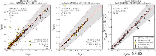
All: the normalized median absolute deviation of source redshifts (σNMAD), the catastrophic outlier fraction (F) where Δz/(zspec+1) ≤ 15 per cent and the number of points included in the sample (N). Left: a photometric versus spectroscopic redshift comparison for radio-detected objects in either ZFOURGE (yellow diamonds) or NMBS (orange diamonds). Ks-selected objects with available spectroscopic redshifts from ZFOURGE are shown for reference (black circles). A 1:1 line is also plotted (solid, red) along with the Δz/(zspec+1) ≤ 15 per cent limits for reference (grey area). Centre: a photometric versus spectroscopic redshift comparison for radio objects detected in both ZFOURGE and NMBS. Right: a photometric versus photometric redshift comparison for radio objects detected in both ZFOURGE and NMBS (grey diamonds). While ZFOURGE in general suffers a slightly higher outlier fraction than NMBS in the leftmost panel, this is largely due to a small population of poorly fitted faint sources that are undetected in NMBS. These sources are flagged and are not included in our analysis.
Overall, ZFOURGE and NMBS produce redshifts with errors of just 1–2 per cent (normalized median absolute deviation, NMAD; Whitaker et al. 2011; Tomczak et al. 2014; Yuan et al. 2014) and are comparably accurate for radio-detected objects (Fig. 1, left). However, radio-detected objects show a higher catastrophic failure rate from template mismatches and SED variability, which may be due to significant contamination of the stellar light by AGN emissions. Indeed, for the six radio-detected photometric redshift outliers, two objects have the smooth power-law SED shape associated with optical AGN, one shows strong variability in the NIR (indicating potential IR-AGN activity) and the remaining three have poorly fitted SEDs due to coverage issues in some bands. These objects are removed during our flagging stages.
Fig. 1 (centre) shows a photometric versus spectroscopic redshift analysis limited to only those objects with detections in both surveys. Here we can see good agreement and comparable accuracy between ZFOURGE and NMBS out to z ∼ 1.0. The absence of high-redshift spectra means we cannot directly test the accuracy of our photometric redshifts at values much higher than z ∼ 1.0, but we draw attention to the fact that both ZFOURGE and NMBS are specifically designed to produce accurate redshifts in the 1.5 < z < 2.25 regime for galaxies with strong 4000 Å/Balmer breaks. The majority of our z > 1.0 radio galaxies have red SEDs with strong breaks similar to those shown in Fig. 2 and overall are well fitted by the stellar templates. Finally, we note that the photometric redshifts from both surveys show good agreement with spectroscopic redshifts out to z ∼ 1.5 and with each other out to z ∼ 3 (Fig. 1, right).
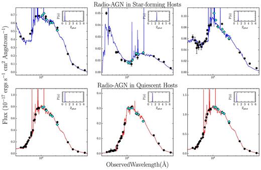
Example SED fits for two of our radio-detected populations: radio-AGN with quiescent hosts and radio-AGN with star-forming hosts (defined in Figs 5 & 6). Photometric data points from ZFOURGE are shown (light blue) along with additional photometric data from other surveys used in the fitting process (black); error bars are also shown. The best-fitting eazy SEDs are shown, colour-coded by their UVJ colour-code classification: quiescent (red) or star-forming (blue). In each panel, a sub-plot displays the eazy calculated probability distribution across redshift with narrow P(z) functions (in blue) indicating reliable photometric redshift fits. We can see that both types of radio-AGN hosts show good photometric fits, and note that this is representative of the samples in general. Spitzer/MIPS 24 μm fluxes were not used in the SED fitting process.
2.2 1.4 GHz radio observations
Radio detections in the CDF-S field are determined from the images and catalogues of the Very Large Array (VLA) 1.4 GHz Survey of the Extended Chandra Deep Field-South: Second Data Release (Miller et al. 2013). Covering an area approximately a third of a square degree with an average rms of 7.4 μJy beam−1, this survey covers the entirety of ZFOURGE Ks-band observations in the CDF-S and has an excellent angular resolution of 2.8 arcsec by 1.6 arcsec.
Radio detections for the COSMOS field are taken from the 1.4 GHz VLA COSMOS Deep project (Schinnerer et al. 2010) which has an rms of 10 μJy beam−1. The COSMOS Deep project covers the entirety of the ZFOURGE and NMBS Ks/K-band observations with an angular resolution of 2.5 arcsec × 2.5 arcsec.
2.3 Cross-matching radio and K-band catalogues
To check the astrometry between radio and Ks images, we cross-match our catalogues using a 5 arcsec separation radius and calculate the average positional offset. The COSMOS and CDF-S ZFOURGE images are found to have systematic astrometric discrepancies of 0.15 and 0.30 arcsec, respectively, when compared to the 1.4 GHz observations. The NMBS data show only a 0.08 arcsec offset from the COSMOS 1.4 GHz field. We apply corrections for these offsets in all subsequent cross-matching.
We now determine the separation at which we will assume that radio and Ks sources are associated by calculating the number of radio–Ks pairs as a function of angular separation (0–5 arcsec) for both N0MBS and ZFOURGE.
To remove the effects of chance alignments, we create a model of randomly positioned, point-like sources and subtract this model from the observed distribution. The resultant distribution is largely Gaussian with 68 per cent of radio–Ks pairs separated by less than 0.32 arcsec (Fig. 3) for ZFOURGE and 0.20 arcsec for NMBS. Due to the quoted 0.3 arcsec accuracy of the Miller et al. (2013) radio catalogues, we therefore adopt a cross-matching radius of 1 arcsec for all fields.
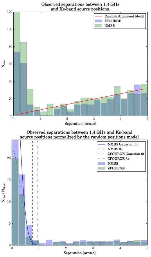
Top: histogram detailing the number of radio to Ks-band pairs as a function of separation for the ZFOURGE (blue) and NMBS (green) surveys. The expectation for randomly positioned, point-like sources shown (red line). Bottom: same as above but normalized by the random expectation model. Gaussians are fitted to the residual ZFOURGE and NMBS populations and their 3σ limits are shown (dotted and dashed vertical lines). We use a 1 arcsec cross-matching radius for both surveys.
Using this limit we cross-match our radio catalogues against Ks/K-band sources with ZFOURGE and NMBS use-flag of 1 which ensures that they have sufficient optical and infrared (IR) imaging coverage, are far away from the scattered light of bright stars and are not stars themselves. We find that 546 radio sources (ZFOURGE: 160 and NMBS: 386) have a Ks-detected counterpart and note that our model for random alignments predicts that less than 14 of these are due to chance (ZFOURGE: 4 and NMBS: 10).
A visual inspection of the cross-matching shows that two objects in the COSMOS field seem to be missed in our automated procedure, despite being well aligned with the head of a head–tail radio galaxy and the core of a Fanaroff–Riley type I radio jet (Fanaroff & Riley 1974). These objects were missed because our selected radio catalogues quote the geometric centre of large, extended objects. We manually add these matches to both the ZFOURGE and NMBS COSMOS sample bringing our total up to 550 (ZFOURGE: 162 and NMBS: 388) radio–Ks pairs. Thus, we detect 550 radio objects in the ZFOURGE and NMBS area, or approximately 91 per cent (550/603) of radio objects that have good coverage in all bands and are not flagged as near stars. The remaining 9 per cent of sources show no Ks-band counterpart within 1 arcsec and are potentially K-band dropouts. We include a list of these objects in Table A3.
We further flag our sample to ensure sensible handling of the overlapping NMBS and ZFOURGE fields, to minimize the difference in radio sensitivity between fields and to catch any poor SED fits missed by the automated procedure (Table 1).
Flagging breakdown, the number of sources remaining in the catalogues after applying each flagging stage.
| Radio sources | NMBS | ZFOURGE |
|---|---|---|
| With Ks-counterpart | 388 (91 ± 2 per cent) | 162 (89 ± 2 per cent) |
| Post-F1.4 < 50 μJy flag | 381 | 115 |
| Post-duplicate flag | 317 | 115 |
| Post-SED flag | 312 | 107 |
| Radio sources | NMBS | ZFOURGE |
|---|---|---|
| With Ks-counterpart | 388 (91 ± 2 per cent) | 162 (89 ± 2 per cent) |
| Post-F1.4 < 50 μJy flag | 381 | 115 |
| Post-duplicate flag | 317 | 115 |
| Post-SED flag | 312 | 107 |
To do this, we flag all objects with 1.4 GHz fluxes less than 50 μJy in order to keep our radio sensitivity constant across all fields. This reduces our radio sample down to 496 objects (ZFOURGE: 115 and NMBS: 381).
Some NMBS and ZFOURGE sources are the same due to the overlapping observations. Inside the overlapping region between NMBS and ZFOURGE, we preferentially use ZFOURGE data wherever possible as the greater signal-to-noise should result in more secure redshift fitting for dusty star-forming and quiescent objects (which dominate our sample) at redshifts greater than 1.5. If, however, any radio detection does not have a ZFOURGE counterpart, for example due to flagging or sensitivity issues, it will have been included in the analysis wherever possible via the NMBS observations. Outside the overlapping region, we use NMBS exclusively. After duplicate flagging, there remain 432 objects with reliable Ks/K- and radio-band detections shared between ZFOURGE and NMBS (Tables A1 and A2). The Ks/K-band, radio luminosity and stellar-mass distributions of this sample are shown in Fig. 4.
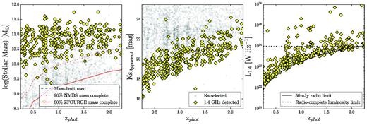
Stellar mass, Ks magnitude and 1.4 GHz luminosities against zphot for the combined ZFOURGE and NMBS fields. The entire Ks-band selected sample is shown (black circles), alongside the 424 Ks-band objects with a 1.4 GHz counterpart within 1 arcsec (yellow diamonds). Left: the mass distribution of our galaxy sample shows a clear bias for radio detections to be found in massive galaxies. To account for this mass bias and to allow ready comparisons between radio-detected and radio non-detected sources, we define our mass-limited sample as objects above 1010.5 M⊙ (red dashes) and note that this is above both the 80 per cent ZFOURGE mass completeness limit (red line; Papovich et al. 2015) and the 90 per cent NMBS mass completeness limit, which is the ZFOURGE 90 per cent curve scaled to match the quoted z = 2.20 (red dot–dashed line; Wake et al. 2011) out to our redshift limit of z = 2.25. Centre: the Ks magnitude distribution as a function of redshift for 1.4 GHz radio detections. Right: 1.4 GHz luminosities as a function of redshift along with our luminosity completeness limit of 1024 W Hz−1 out to a redshift of z = 2.25. Note that for clarity only 10 per cent of the radio non-detected sources are plotted.
Finally, we manually flag 13 objects due to poorly fitted SEDs. Two of these objects are flagged due to saturated or missing coverage that is missed by the automated flagging due to the averaging of sensitivity coverage over 1.2 by 1.2 arcsec areas. Of the remaining 11 sources, 7 possess pure power-law SEDs whose redshift estimate cannot be trusted as there is no break in the SED for eazy to fit too and 4 SEDs showing large variability between observations in the NIR bands. Hence, we have flagged 2.5 per cent of our final radio sample due to poor SED fits.
3 CLASSIFYING RADIO GALAXIES
3.1 By host type
We determine the stellar population properties, including mass, dust content, rest-frame colours and luminosities of our sample, by fitting Bruzual & Charlot (2003) stellar population synthesis models with fast (Kriek et al. 2009) using a Chabrier (2003) initial mass function. Fig. 3 shows example SEDs and fits. Finally, galaxies were divided into two stellar population types: quiescent or star-forming, based upon their UVJ position (Wuyts et al. 2007), shown in Fig. 5.
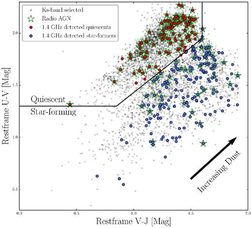
The rest-frame, UVJ colour–colour diagram for radio-detected star-formers (blue circles), radio-detected quiescent galaxies (red circles) and the ZFOURGE Ks-band mass-limited sample (black circles). Radio-AGN are selected based on their radio-to-UV+24 μm SFR ratios and are highlighted (green stars). For clarity, only 10 per cent of the radio non-detected sources are plotted.
3.2 By radio-AGN activity
A large number of techniques are currently used to identify radio-AGN [see Hao et al. (2014) for a review of nine separate methods], but a key indicator is the ratio of 24 μm to 1.4 GHz flux or the ratio of far-infrared (FIR, 70–160 μm) to 1.4 GHz flux. The resultant tight linear correlation shows no evolution out to a redshift of 2 (Mao et al. 2011) and is commonly known as the FIR radio correlation. Objects lying significantly off this correlation are typically classified as radio-AGN but the offset required for this depends on the AGN SED model and redshift.
It has been suggested that low-redshift, radio-quiet AGN are dominated in radio wavelengths by host galaxy star formation (Kimball et al. 2011; Bonzini et al. 2013), and composite sources in which AGN and star formation both contribute to the radio emission are well known (Emonts et al. 2011, 2014; Carilli & Walter 2013). We therefore define a radio-AGN as an object in which the total radio flux is significantly greater than the radio emission expected from the SFR determined at other wavelengths.
This SFR allows for the accurate tracing of star formation in a non-dusty host via UV emissions from hot young stars and complements this with the contribution from dust-obscured stars using 24 μm observations.
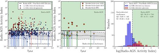
Left: the ratio of UV+IR to radio SFR as a function of redshift, colour-coded by stellar population type. Objects with 24 μm fluxes less than the 24 μm sensitivity are shown as 3σ lower limits (arrows). The Wuyts et al. (2008) average star-forming galaxy SED template is shown (thin black line) along with the 3σ scatter seen the 1.4 GHz-to-24 μm flux ratios of local star-forming galaxies (grey shaded area). We determine that objects above the upper limit of this line (i.e. SFR1.4 GHz/SFRUV+IR ≥ 3.0) are considered to be radio-AGN (green shading). Centre: a comparison of our classification of radio-AGN and non-radio-AGN sources to the Bonzini et al. (2013) classification scheme: radio-loud AGN (dark orange squares), radio-quiet AGN (light orange circles) and radio-detected star-forming galaxies (light blue triangles). We see good agreement between Bonzini radio-loud AGN and our radio-AGN sample. Right: a breakdown of combined UV+24 μm to radio SFR ratios as a function of quiescent (red) or star-forming (blue) host galaxies. The breakdown of host types for radio-AGN (green shaded) and radio-detected star-formers (white shaded) is labelled.
We use the Wuyts et al. (2011) average star-forming template to predict the expected indices of star-forming galaxies. The Wuyts template produces a nearly flat ratio of SFRs which is only slightly dependent upon redshift; hence, we approximate the dividing line between star-formation-driven radio emission and AGN-driven radio emission as three times the scatter seen in local 1.4 GHz-to-FIR flux ratios (0.39 dex; Morić et al. 2010). This divides our radio-detected sample into two: objects whose radio-AGN activity index is less than 3.0 are henceforth classified as radio-detected star-formers and those whose radio-AGN activity index is greater than 3.0 are classified as radio-AGN. Fig. 6 (centre) compares our radio-AGN selection criteria to that of Bonzini et al. (2013). We see good agreement between our radio-AGN sample and their sample of radio-loud AGN. Finally, we note that our results do not change significantly if our radio-AGN selection criteria are raised from a radio-AGN activity index of 3.0, up to an index of 5.0. The breakdown of quiescent and star-forming hosts as a function of our radio-AGN selection criteria is shown in Fig. 6 (right).
While the combined UV+IR SFR should give a good estimate of total SFR, independent of dust obscuration for the majority of sources, it does, however, assume that the entirety of the observed 24 μm flux is from star formation and not contaminated by a hot, dusty AGN torus. To determine how much of an impact this issue will have on our analysis, we apply the Donley colour wedge (Donley et al. 2012) to our final analysis sample to determine the number of radio sources with IR-AGN colours. We find that 10 ± 2 per cent (40/412) radio-detected objects in our sensitivity-limited sample have IR-AGN colours, and note that these objects may have artificially elevated SFRs.
But how does AGN contamination of the 24 μm flux affect our analysis of specific star formation rates (SSFRs) in radio-AGN and mass-similar galaxies? Of the 40 IR AGN identified, only 10 fall within our final mass- and radio-luminosity-complete sample of 65 objects (15|$^{+5}_{-3}$| per cent) and only 4 of these are also classified as radio-AGN (of which there are 42). If we remove these objects from our radio-AGN analysis, along with every identified IR-AGN candidate from the mass- and luminosity-complete control sample of non-radio-AGN, we find no significant change in our findings.
Due to the presence of IR AGN, it is also possible that we misclassify a fraction of radio-AGN as radio star-formers due to contamination of the 24 μm flux. Any IR flux from an AGN will artificially inflate the host galaxies’ SFRUV+IR estimate, potentially keeping it below the division in Fig. 6 (left). Because of this, it is possible that with better FIR observations some sources may move upwards from their current positions in Fig. 6 (left) and become re-classified as radio-AGN. To quantify the how common these objects are, we calculate the number of IR AGN in the mass- and radio-luminosity-complete sample that are not currently classified as radio-AGN. It is possible that these six objects should be included in our radio-AGN sample. Therefore, we estimate that our radio-AGN sample is at worst 88|$^{+3}_{-6}$| per cent (42/(42+6)) complete due to this effect, and note that the inclusion of these objects in our analysis makes no significant changes to our findings.
To account for these effects, the upper error bar on the quoted radio-AGN fraction for the sensitivity-limited sample given in Section 4.1 includes the value we attain should all 40 of the IR AGN in the sensitivity-limited sample currently identified as radio-detected star-formers were to move into our radio-AGN sample. The equivalent has been done for our AGN fraction versus redshift analysis shown in Fig. 12.
4 ANALYSIS
4.1 The radio sensitivity-limited sky
The upcoming deep radio survey the Evolutionary Map of the Universe (EMU) will observe approximately 75 per cent of the radio sky down to a limiting 5σ sensitivity of 50 μJy and produce a catalogue of approximately 70 million radio galaxies (Norris, Hopkins & Afonso 2011). To prepare for this large undertaking, we now characterize the radio sky at a comparable sensitivity to EMU.
The majority of radio objects (76 per cent) are found to have rest-frame UVJ colours associated with actively star-forming galaxies. Notably, the star-forming radio population shows a significant bias towards high dust content, with V − J values typically above the dusty, non-dusty border at V − J = 1.2 (Spitler et al. 2014).
Radio sources are found to have a median mass of 1010.8 ± 0.5 M⊙, a median redshift of z = 1.0 ± 0.7, a median SSFR of 0.8 ± 3.7 M⊙ Gyr−1 and a median visual extinction of 1.4 ± 0.9 mag. The errors quoted here are the standard deviations as we are characterizing the populations rather than constraining the medians. We determine that only 38|$^{+6 }_{ -2}$| per cent of radio sources (1σ beta confidence interval error; Cameron 2011) above 50 μJy are radio-AGN, and this fraction shows no evolution within errors in the redshift range of 0.25–2.25. This confirms the result by Seymour et al. (2008) that the sub-mJy radio sky is dominated by emissions from star formation.
4.2 The mass-limited and mass-similar, radio-complete sky
We now limit our sample in terms of mass, radio luminosity and redshift to allow for a fair comparison between high-mass radio galaxies and their non-radio counterparts using the following criteria.
0.25 ≤ z < 2.25 to minimize the effects of our small survey volume and ensure completeness in both radio luminosity and mass.
Radio luminosities greater than 1024 W Hz−1 at 1.4 GHz observed. Objects above this limit are referred to hereafter as high-luminosity sources and objects below this limit as low-luminosity sources.
In addition, we produce two slightly different control samples.
The ‘mass-similar’ population is used for comparing the properties of our test groups (both radio-AGN and radio-detected star-forming galaxies) to a control sample comprised of galaxies with similar redshifts and mass. In each case, we determine the number of objects within our test population and randomly select the same number of Ks-detected galaxies from within each of our redshift bins (0.25–1.00, 1.00–1.65 and 1.65–2.25) whose stellar masses are within 0.1 log(M⊙) of an object in the test group. We then measure and record the median value for each property of interest (e.g. SFR) for this mass-similar control population and repeat the process 1000 times. The median value of all these measurements is then compared to the median of the test population (radio-AGN or radio-detected star-formers). Errors on all test population properties are standard errors and errors on the mass-similar control samples are calculated using the NMAD of the 1000 random samples.
The ‘mass-limited’ population is simply all objects with stellar masses greater than 1010.5 M⊙ (Fig. 4, left) and used solely for determining the fraction of galaxies containing a radio-AGN.
Both our mass-similar and mass-limited samples are above the mass completeness limit for the both the ZFOURGE (80 per cent limit = 7.8 × 10⁹ M⊙; Papovich et al. 2015) and NMBS (90 per cent limit = 3.0 × 1010.0 M⊙; Wake et al. 2011; Brammer et al. 2011) surveys at our maximum redshift of z = 2.25. Finally, all percentage and fraction errors in this paper are 1σ values calculated using the beta confidence interval (Cameron 2011).
4.2.1 Radio-detected star-formers
We now consider radio galaxies whose radio-AGN activity index is less than 3.0 (i.e. objects whose radio emissions are consistent with what we would expect to detect based on their SFR). In Fig. 5, we see that these high-luminosity ‘radio-detected star-formers’ are associated with star-forming rest-frame UVJ colour (91|$^{+3}_{-10}$| per cent) and that the 9 per cent of these objects found in the quiescent UVJ region are located very near the quiescent–star-forming boundary. Of these two objects, we find that one has an X-ray detection in public catalogues. In general, these objects are thought to have simply scattered outside the UVJ star-forming region, but it is also possible that we are seeing the last effects of residual star formation in a largely quiescent host.
As a whole, we find high-luminosity radio-detected star-forming galaxies to possess higher SFRs (P < 0.01) than their mass- and redshift-similar star-forming counterparts (Table 2) andx we note that the low Kolmogorov-Smirnov Test (KS-test) P-value for this property is likely due to the sensitivity bias of our radio observations towards high-luminosity (and hence high-SFR) sources.
Median properties for the 23 ‘radio-detected star-former’ galaxies (median L1.4 GHz = 1.34 × 1024 W Hz−1) in ZFOURGE and NMBS, compared against the mass-similar, redshift binned radio non-detected star-former sample.
| Property | Radio-detected | Mass-similar | KS P-value |
|---|---|---|---|
| log(mass) (M⊙) | 11.03 ± 0.06 | 11.00 ± 0.02 | 0.98 |
| Redshift | 1.68 ± 0.06 | 1.54 ± 0.16 | 0.10 |
| SSFR (M⊙ Gyr−1) | 3.92 ± 0.59 | 0.78 ± 0.21 | 0.00 |
| Visual extinction (mag) | 1.60 ± 0.14 | 1.40 ± 0.19 | 0.36 |
| Property | Radio-detected | Mass-similar | KS P-value |
|---|---|---|---|
| log(mass) (M⊙) | 11.03 ± 0.06 | 11.00 ± 0.02 | 0.98 |
| Redshift | 1.68 ± 0.06 | 1.54 ± 0.16 | 0.10 |
| SSFR (M⊙ Gyr−1) | 3.92 ± 0.59 | 0.78 ± 0.21 | 0.00 |
| Visual extinction (mag) | 1.60 ± 0.14 | 1.40 ± 0.19 | 0.36 |
4.2.2 Radio-AGN
While low-redshift radio-AGN are traditionally associated with massive ellipticals (Lilly & Prestage 1987; Owen & Laing 1989; Véron-Cetty & Véron 2001), our sample shows a variety of rest-frame colours, with only 48 ± 7 per cent of high-luminosity radio-AGN found within quiescent galaxies (Table 2). The remaining 52 ± 7 per cent are hosted in star-formers with high dust contents which is in good agreement with the growing number of CO detections found in high-z radio galaxies (Emonts et al. 2011, 2014; Carilli & Walter 2013).
Quiescent galaxy hosts with high-luminosity radio-AGN are found to possess SFRs and dust contents indistinguishable from the mass-similar quiescent population (P = 0.56 and 0.82, respectively, see Table 3). Fig. 7 shows no evidence to suggest either suppressed or enhanced star formation in our redshift range of 0.25–2.25.

The measured median values for mass (top), SSFR (middle) and visual extinction (bottom) for high-luminosity, quiescent and star-forming radio-AGN compared to their mass-similar counterparts. We see no evidence for enhanced or suppressed star formation in high-luminosity radio-AGN hosts within our redshift range. Errors are standard errors on the median and the NMAD, for radio-AGN and the mass-similar sample, respectively. Values are offset by 0.10 in the horizontal direction for clarity.
Median properties for the 22 radio-AGN in quiescent hosts (median L1.4 GHz = 3.1 × 1024 W Hz−1) in ZFOURGE and NMBS, compared against the mass-similar, redshift binned, non-AGN quiescent population.
| Radio-AGN | No radio-AGN | ||
|---|---|---|---|
| Property | (QU) | (QU) | KS P-value |
| log(mass) (M⊙) | 11.14 ± 0.06 | 11.12 ± 0.02 | 0.98 |
| Redshift | 1.10 ± 0.13 | 0.99 ± 0.16 | 0.56 |
| SSFR (M⊙ Gyr−1) | 0.08 ± 0.13 | 0.06 ± 0.02 | 0.56 |
| Visual extinction (mag) | 0.55 ± 0.10 | 0.50 ± 0.09 | 0.82 |
To determine the evolving stellar (and corresponding fixed halo) mass at which high-luminosity radio-AGN appear, we plot the masses of radio-AGN as a function of redshift (see Fig. 8). Comparing these observations to a fixed halo mass, which has been converted to stellar mass using the Moster et al. (2010) stellar-to-halo mass relation (Moster et al., equation 24), we determine the halo mass that bounds the high-luminosity radio-AGN population to be 1012 M⊙.
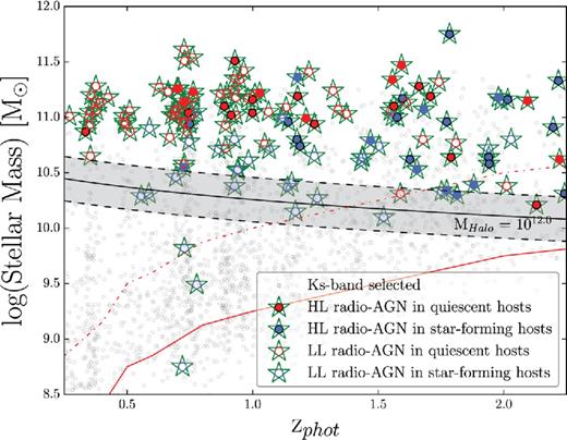
The stellar masses of high- (L1.4 ≥ 1024 W Hz−1) and low-luminosity (L1.4 ≤ 1024 W Hz−1) radio-AGN. (filled and open circles with green stars, respectively). Quiescent and star-forming host types are also shown (red and blue circles, respectively). The stellar-mass equivalent of a 1012 M⊙ halo mass (black line) along with the Ks-selected sample (black circles) is plotted for reference; for clarity only 10 per cent of the Ks-selected sample is plotted. Finally, the 80 per cent ZFOURGE mass completeness limit is shown (red line; Papovich et al. 2015) along with the 90 per cent NMBS mass completeness limit, extrapolated down from z = 2.20 (red dot–dashed line; Wake et al. 2011). Radio-AGN in quiescent hosts are only found in objects with halo masses above 1012 M⊙ (black line); 100 per cent of high-luminosity radio-AGN in our sample are found above this line. The 1σ local scatter in the stellar-to-halo mass relation is shown (grey shaded region). Finally, we note that for this plot we do not limit our radio-AGN sample by mass in any way.
Of our high-luminosity radio-AGN, 20 are found to be embedded within star-forming hosts (‘composites’ hereafter). These sources contain large amounts of dust and would be easy to misclassify as quiescent without the use of our medium band NIR filters (J1, J2, J3, Hs and Hl). Comparing composites to the star-forming population, we see in Fig. 9 that a small number show extremely high SFR and SSFRs and are undoubtedly undergoing a starburst phase. Despite this, Fig. 7 shows that overall the SFRs and dust content of composite sources remain consistent with the mass-similar star-forming population (P = 0.13 and 0.77, respectively). A visual inspection of Fig. 10 shows that of the eight composites covered by Hubble Space Telescope (CANDELS; Grogin et al. 2011), seven have nearby companions and three show clear tidal interactions (objects 4, 5 and 8). However, these three sources do not correspond with any of the starbursting objects visible in Fig. 9 (bottom). Additionally, four composites are found to have strong X-ray counterparts with hardness ratios indicative of efficient accretion on to an AGN (Cowley et al., submitted) but also show no signs of elevated SSFRs. Finally, the high-luminosity composite population visible in ZFOURGE shows disc-like morphologies with a median Sérsic index of 1.76 ± 0.18 (van der Wel et al. 2014).

Top: the mass–redshift relation for high-luminosity radio-AGN in star-forming hosts (blue circles with green stars) and high-luminosity radio-AGN in quiescent hosts (red circles with green stars). For reference, the Ks-selected sample is also shown (grey circles) along with the mass limit used for our analysis of the various populations (red dashed line). For clarity, only 10 per cent of the Ks-selected sample is plotted. Middle: the mass versus SFR plot. Bottom: the mass versus SSFR plot.
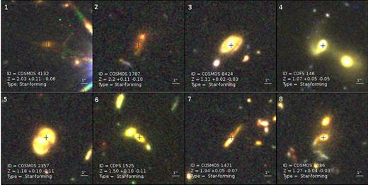
RGB thumbnails of composite sources using F125W, F160W and F814W filters; three sources show sure signs of merger activity (4, 5 and 8), and 7/8 show nearby companions or distorted morphologies (with the exception of composite 1).
Studying the evolution of high-luminosity radio-AGN as a whole, we can see that in terms of UVJ colour, radio-AGN hosts evolve with redshift in a manner that is indistinguishable from their mass-similar, non-radio-AGN counterparts (Fig. 11).
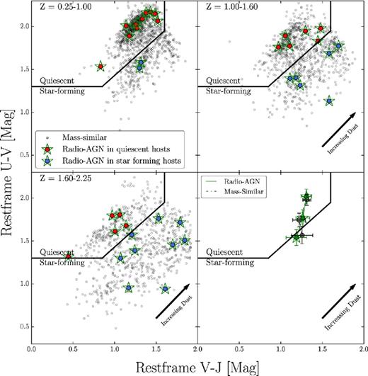
The UVJ diagram for high-luminosity radio-AGN compared to the mass-similar sample in three redshift bins: 0.25–1.0 (top left), 1.0–1.60 (top right) and 1.60–2.25 (bottom left). Bottom right: the median position for radio-AGN and the randomly sampled mass-similar population across the three redshift bins. Errors are standard errors on the median and the NMAD, respectively. For clarity, only 10 per cent of the Ks-selected sample is plotted.
Fig. 12 (left) shows the fraction of galaxies containing a high-luminosity radio-AGN as a function of redshift. We find that across our full redshift range, an average of 1.0|$^{+0.3}_{-0.2}$| per cent of quiescent, 1.1|$^{+0.3}_{-0.2}$| per cent of star-formers and only 1.0|$^{+0.3}_{-0.1}$| per cent of all massive galaxies (M ≥ 1010.5 M⊙) host a high-luminosity radio-AGN, with little evolution in these values as a function of redshift. In Fig. 12 (centre), we see a tight dependence between high-luminosity radio-AGN and stellar mass, with a significant decrease in the abundance of these objects from approximately 10 per cent at M ≥ 1011.5 M⊙ down to less than 1 per cent at M ≥ 1010.5 M⊙. We draw attention to the sharp drop-off seen in Fig. 12 (right) where the fraction of star-forming high-luminosity radio-AGN hosts declines rapidly below a redshift of z = 1.5. This is consistent with the declining percentage of high-mass galaxies that are star-forming in general, within our mass-limited sample. This may explain the rarity of low-redshift composites as simply due to the lack of suitable high-mass star-forming galaxies in the local Universe. Finally, we note that in Fig. 12 (left and right), the star-forming and quiescent high-luminosity radio-AGN fractions follow the same trend within errors.
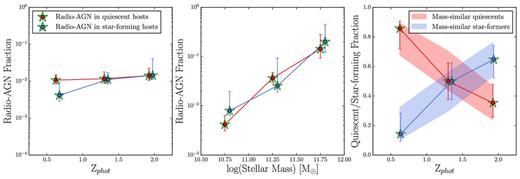
Left: the evolving radio-AGN fraction for quiescent (red with green stars) and star-forming (blue with green stars) high-luminosity radio-AGN above our mass limit of 1010.5 M⊙. Centre: the radio-AGN fraction for each host type as a function of stellar mass shows a sharp drop-off in radio-AGN fraction as we progress to lower masses in excellent agreement with Best et al. (2005). Left and centre panels show the number of quiescent or star-forming radio-AGN hosts divided by the number of quiescent of star-forming galaxies in the given bin. Right: the breakdown of quiescent and star-forming high-luminosity radio-AGN hosts as a function of redshift. The fraction of quiescent (red shaded) and star-forming (blue shaded) galaxies of similar masses to the radio-AGN hosts is shown for comparison. All errors are beta confidence intervals and NMAD errors from 1000 random samples for the radio-AGN and mass-similar samples, respectively.
5 DISCUSSION
Using our high-luminosity (L1.4 > 1024 W Hz−1) mass-limited radio-AGN sample, we are able to study the fraction of massive galaxies that host radio-AGN to a redshift of z = 2.25. Fig. 8 shows that high-luminosity radio-AGN become rare beneath a stellar-mass limit of ∼1010.5 M⊙ at low redshifts (z = 0.25). Interestingly, this limit evolves with time, such that it mimics the expected evolution of the stellar-to-halo mass relation for a fixed halo mass of 1012 M⊙. The implication of this result is that there may be a link between galaxies with high-mass haloes and the triggering of high-luminosity radio-AGN. Indeed, the apparent halo-mass limit for hosting radio-AGN is consistent with the critical halo mass at which simulations typically have to invoke AGN feedback in order to reproduce the local galaxy mass function (Springel et al. 2005; Croton et al. 2006).
As seen in Fig. 8, only a small number of high-luminosity radio-AGN fall below our 1012 M⊙ halo-mass line [converted to stellar mass using the Moster et al. (2010) stellar-to-halo mass relation]. At z > 1, this may be partially due to the incompleteness of NMBS below 1010.5 M⊙. However, even at z < 1, where our completeness is well above 80 per cent, we see very few radio-AGN in low-mass galaxies. Assuming that this halo mass is required for powerful radio-AGN activity, the few objects that are found in lower mass galaxies may reflect scatter in the stellar-to-halo mass relation (≃0.2 dex at z = 0; More et al. 2009; Yang, Mo & van den Bosch 2009; Behroozi, Wechsler & Conroy 2013; Reddick et al. 2013). In addition to this, Kawinwanichakij et al. (2014) find that quiescent galaxies at high redshift have unusually large halo masses for a given stellar mass (by up to ≃0.1–0.2 dex); hence, it is possible that some of our low-mass radio-AGN hosts may actually reside in haloes larger than the Moster et al. median.
Alternatively, the observed halo-mass limit we discussed above may simply correspond to the stellar mass where the high-luminosity radio-AGN fraction becomes negligible. Fig. 12 (left and centre) shows the fraction of massive galaxies containing a high-luminosity radio-AGN as a function of redshift and mass. While we find little evolution in the high-luminosity radio-AGN fraction as a function of redshift, we do observe a strong correlation with stellar mass. Fig. 13 shows a comparison between the mass-dependent radio-AGN fraction of our study and those of previous work in three redshift bins: 0.4 < z < 0.8, 0.8 < z < 1.2 (to match previous studies) and 1.2 < z < 2.25. Our high-luminosity radio-AGN fraction is slightly higher than that found in previous studies (0.03 < z < 0.1, Best et al. 2005 and 0.4 < z < 1.2, Simpson et al. 2013), and we speculate that this may be due to differences in the techniques used to identify our radio-AGN samples. Despite this offset, the lack of evolution between redshift bins in our study is consistent with the lack of evolution seen between redshifts in these previous investigations. This raises the question of whether the universal radio-AGN fraction is simply a function of stellar mass, with the most massive galaxies being much more likely to host radio-AGN activity than low-mass galaxies. In extremity, extrapolating upwards in stellar mass suggests that above stellar masses of 1012 M⊙, nearly all galaxies should contain a radio-AGN.
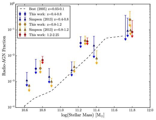
The fraction of galaxies containing radio-AGN with luminosities greater than 1024 W Hz−1 as a function of mass for three redshift bins: 0.4 < z < 0.8 (blue circles), 0.8 < z < 1.2 (orange circles) and 1.2 < z < 2.25 (red circles). We see no evolution between our redshift bins. This is in good agreement with previous studies by Best et al. (2005) at 0.03 < z < 0.1 (black dashes) and Simpson et al. (2013) at 0.4 < z < 0.8 (blue triangles) and 0.8 < z < 1.2 (orange triangles). Our low-mass radio-AGN fraction is elevated at all redshifts compared to previous studies, which may be due to differences in how we select our radio-AGN samples.
To investigate the impact of radio-AGN on host galaxy properties, we also use our mass-similar sample to compare radio-AGN hosts to non-hosts. We find that the high number of close companions and mergers seen in our high-luminosity composite (radio-AGN in star-forming hosts) sample seems to support a merger-driven AGN triggering model. Despite this, we see no evidence for the enhanced SFRs expected during merger scenarios (Table 4) as composite SFRs are indistinguishable from the mass-similar star-forming sample. This may only reflect the short time-scales of a merger-induced starburst. Finally, Fig. 12 (right) shows that the fraction of radio-AGN hosted within quiescent and star-forming hosts evolves in a similar fashion to the non-AGN galaxy population. These results suggest that the radio-AGN and non-radio-AGN populations are hosted by galaxies with similar properties.
Median properties for the 20 radio-AGN in star-forming hosts (median L1.4 GHz = 2.7 × 1024 W Hz−1) in ZFOURGE and NMBS, compared against the mass-similar, redshift binned, non-AGN star-forming population.
| Property | Radio-AGN | No radio-AGN | KS P-value |
|---|---|---|---|
| (SF) | (SF) | ||
| log(mass) (M⊙) | 10.95 ± 0.09 | 10.92 ± 0.03 | 0.97 |
| Redshift | 1.64 ± 0.12 | 1.55 ± 0.16 | 0.50 |
| SSFR (M⊙ Gyr−1) | 1.41 ± 0.96 | 0.79 ± 0.25 | 0.13 |
| Visual extinction (mag) | 1.45 ± 0.16 | 1.45 ± 0.21 | 0.77 |
6 CONCLUSIONS
We have combined a deep Ks-band selected sample, which is ideal for selecting galaxies across a wide redshift range (Rocca-Volmerange et al. 2013) with high-quality photometric redshifts and sensitive 1.4 GHz VLA observations to identify 412 radio sources in the CDF-S and COSMOS legacy fields. This sample is split into two sub-groups: radio-AGN and radio-detected star-forming galaxies using the ratio of the UV+24-μm-based and radio-based SFRs. Using this sample, we study the host properties of radio-AGN and compare them to a non-radio sample of similar masses and redshifts out to a redshift of 2.25.
We find that the fraction of galaxies that contain radio-AGN at a given stellar mass shows little dependence on redshift or star formation activity. This is in good agreement with the findings of Best et al. (2005) and Simpson et al. (2013) and extends the analysis of radio-AGN fractions to higher redshift ranges than previously explored.
The type of galaxies that host radio-AGN shows strong evolution as a function of redshift, from predominantly dusty, star-forming hosts in interacting or merger environments (1 < z < 2.25) to predominantly quiescent hosts at z < 1.
This evolution is in line with the overall evolution of massive galaxies on to the red sequence.
The above findings are in good general agreement with earlier work, particularly that of Rocca-Volmerange et al. (2013) and De Breuck et al. (2002).
Radio-AGN become particularly rare at halo masses below 1012 M⊙, suggesting that radio-AGN activity may be closely linked to high halo masses.
Finally, our radio-AGN hosts show SFRs and SSFRs consistent with non-radio-AGN hosts of similar mass and redshift, in good agreement with earlier work out to z ∼ 0.7 (Johnston et al. 2008; Chen et al. 2013).
In summary we find that radio-AGN hosts show no statistical differences from non-hosts across a broad redshift range (0.25 ≤ z < 2.25) and that the fraction of galaxies containing radio-AGN at a given stellar mass is independent of both redshift and host type. Ultimately, by including these observations into models of AGN feedback and triggering, we hope that new insights may be gained into how these powerful objects both form and evolve.
We would like to thank the Mitchell family for their continuing support of the ZFOURGE project. We would also like to thank the Carnegie Observatories and the Las Campanas Observatory for providing the facilities and support needed to make ZFOURGE what it is today. Australian access to the Magellan Telescopes was supported through the National Collaborative Research Infrastructure Strategy of the Australian Federal Government. This research has made use of NASA's Astrophysics Data System. This research has also made use of the NASA/IPAC Extragalactic Database (NED) which is operated by the Jet Propulsion Laboratory, California Institute of Technology, under contract with the National Aeronautics and Space Administration. This research made use of aplpy, an open-source plotting package for python hosted at http://aplpy.github.com. This research also made use of astropy, a community-developed core python package for Astronomy (Robitaille et al. 2013). This work made use of the ipython package (Pérez & Granger 2007). This research made use of matplotlib, a python library for publication quality graphics (Hunter 2007). pyraf is a product of the Space Telescope Science Institute, which is operated by AURA for NASA. This research made use of scipy (Jones et al. 2001). GGK was supported by an Australian Research Council Future Fellowship FT140100933.
REFERENCES
SUPPORTING INFORMATION
Additional Supporting Information may be found in the online version of this article:
VLA-CDFS-No-Matches.ascii
VLA-COSMOS-No-Matches.ascii
VLA-NMBS-No-Matches.ascii
VLA-NMBS-v1.0.0.ascii
VLA-ZFOURGE-v1.0.0.ascii
Please note: Oxford University Press is not responsible for the content or functionality of any supporting materials supplied by the authors. Any queries (other than missing material) should be directed to the corresponding author for the paper.
APPENDIX A
Extract of the included data set. ‘ID’ is the field and ID of the ZFOURGE Ks-band object, ‘RA’ is the right ascension of the ZFOURGE Ks-band object in decimal degrees, ‘Dec.’ is the declination of the ZFOURGE Ks-band object in decimal degrees, ‘zphot’ is the peak of photometric redshift probability distribution determined by eazy for the ZFOURGE Ks-band object, ‘Mass’ is the logged stellar mass of the ZFOURGE Ks-band object in M⊙, ‘F1.4’ is the 1.4 GHz flux of the ZFOURGE Ks-band object in microjanskys assuming association of sources within 1 arcsec, ‘L1.4’ is the 1.4 GHz luminosity of the ZFOURGE Ks-band object assuming association of sources within 1 arcsec and a spectral index of 0.5 in W Hz, ‘LIR’ is the bolometric IR luminosity of the ZFOURGE Ks-band object assuming a Wuyts et al. (2011) average SED template to extrapolate from 24 μm fluxes, ‘LUV’ is the eazy interpolated rest-frame 2800 Å luminosity of the ZFOURGE Ks-band object, ‘SFRRadio’ is the 1.4 GHz luminosity of the radio object in M⊙ per year, ‘SFRUV+IR’ is the combined SFR from LUV and LIR in M⊙ per year and ‘Type’ is the stellar population type of the Ks-band object based on our rest-frame UVJ colour–colour classification into quiescent (QU) or star-forming (SF) sources. The full table is available online.
| ID | RA | Dec. | Ks-band | zphot | zspec | Mass | F1.4 | L1.4 | LIR | LUV | SFRRadio | SFRUV+IR | SFR ratio | Type |
|---|---|---|---|---|---|---|---|---|---|---|---|---|---|---|
| (deg) | (deg) | (mag) | (M⊙) | (μJy) | (W Hz−1) | (W Hz−1) | (W Hz−1) | (M⊙ yr−1) | (M⊙ yr−1) | |||||
| COSMOS-10055 | 150.147 216 80 | 2.337 183 70 | 19.87 | 0.74 | 0.73 | 10.69 | 67.0 | 1.13e+23 | 9.96e+11 | 1.24e+10 | 3.58e+01 | 1.13e+02 | 0.32 | SF |
| COSMOS-10472 | 150.079 376 20 | 2.340 569 50 | 22.78 | 0.22 | – | 8.21 | 61.0 | 7.58e+21 | 1.42e+10 | 3.76e+07 | 2.41e+00 | 1.57e+00 | 1.54 | SF |
| COSMOS-1055 | 150.057 220 50 | 2.205 927 60 | 18.62 | 0.09 | 0.19 | 9.43 | 446.0 | 9.08e+21 | 4.09e+10 | 2.28e+08 | 2.89e+00 | 4.54e+00 | 0.64 | QU |
| COSMOS-1086 | 150.099 823 00 | 2.203 275 20 | 21.71 | 1.27 | – | 10.75 | 84.0 | 4.44e+23 | 1.27e+11 | 8.16e+09 | 1.41e+02 | 1.68e+01 | 8.42 | SF |
| COSMOS-1096 | 150.056 625 40 | 2.208 554 70 | 18.79 | 0.21 | – | 10.13 | 342.0 | 4.02e+22 | 5.69e+11 | 1.20e+09 | 1.28e+01 | 6.25e+01 | 0.20 | SF |
| COSMOS-11061 | 150.187 973 00 | 2.352 927 40 | 19.50 | 0.27 | – | 10.07 | 90.0 | 1.73e+22 | 7.78e+10 | 8.21e+08 | 5.50e+00 | 8.78e+00 | 0.63 | SF |
| COSMOS-11391 | 150.175 705 00 | 2.358 698 40 | 18.36 | 0.21 | – | 10.51 | 94.0 | 1.10e+22 | 1.23e+11 | 4.08e+09 | 3.50e+00 | 1.49e+01 | 0.23 | SF |
| COSMOS-11542 | 150.085 159 30 | 2.357 328 90 | 20.97 | 1.21 | – | 10.99 | 211.0 | 1.02e+24 | 5.51e+10 | 6.04e+09 | 3.24e+02 | 8.18e+00 | 39.61 | QU |
| COSMOS-11559 | 150.143 035 90 | 2.355 881 70 | 24.20 | 3.00 | – | 10.45 | 517.0 | 1.51e+25 | 1.38e+13 | 2.74e+10 | 4.81e+03 | 1.52e+03 | 3.18 | SF |
Extract of the included NMBS data set. As Table A1. Full table is available online.
| ID | RA | Dec. | Ks-band | zphot | zspec | Mass | F1.4 | L1.4 | LIR | LUV | SFRRadio | SFRUV+IR | SFR ratio | Type |
|---|---|---|---|---|---|---|---|---|---|---|---|---|---|---|
| (deg) | (deg) | (mag) | (M⊙) | (μJy) | (W Hz−1) | (W Hz−1) | (W Hz−1) | (M⊙ yr−1) | (M⊙ yr−1) | |||||
| NMBS-30222 | 149.758 164 71 | 2.181 259 26 | 19.66 | 0.93 | – | 10.76 | 83.0 | 2.60e+23 | 1.02e+11 | 6.16e+09 | 1.44e+02 | 1.30e+02 | 1.11 | SF |
| NMBS-33599 | 150.175 410 90 | 2.426 085 75 | 18.29 | 0.31 | 0.31 | 9.91 | 112.0 | 3.00e+22 | 2.03e+10 | 8.52e+09 | 1.66e+01 | 3.58e+01 | 0.46 | SF |
| NMBS-16854 | 150.007 129 80 | 2.453 478 05 | 18.65 | 0.76 | – | 11.23 | 761.0 | 1.54e+24 | 6.36e+08 | 3.75e+09 | 8.48e+02 | 6.59e+00 | 128.80 | QU |
| NMBS-16644 | 149.850 166 65 | 2.452 232 86 | 19.41 | 0.72 | 0.71 | 10.55 | 1102.0 | 1.98e+24 | 1.17e+10 | 5.65e+09 | 1.10e+03 | 4.78e+01 | 22.91 | SF |
| NMBS-13387 | 150.095 347 01 | 2.384 750 16 | 17.48 | 0.28 | 0.27 | 10.80 | 240.0 | 5.30e+22 | 9.06e+10 | 2.20e+09 | 2.93e+01 | 1.97e+01 | 1.49 | SF |
| NMBS-31704 | 149.860 237 30 | 2.297 592 13 | 20.77 | 1.83 | – | 11.12 | 68.0 | 9.41e+23 | 5.07e+10 | 2.39e+10 | 5.20e+02 | 3.77e+02 | 1.38 | SF |
| NMBS-11075 | 149.961 434 63 | 2.349 430 35 | 19.14 | 0.93 | – | 11.18 | 230.0 | 7.28e+23 | 2.07e+10 | 5.55e+09 | 4.02e+02 | 4.25e+00 | 94.59 | QU |
| NMBS-2925 | 149.743 113 97 | 2.213 808 15 | 19.04 | 0.87 | 0.89 | 11.21 | 309.0 | 8.41e+23 | 2.21e+10 | 4.11e+09 | 4.64e+02 | 4.91e+00 | 94.65 | QU |
| NMBS-6355 | 149.856 779 87 | 2.273 154 93 | 18.73 | 0.76 | 0.76 | 11.12 | 88.0 | 1.78e+23 | 2.21e+10 | 1.20e+10 | 9.81e+01 | 6.46e+01 | 1.52 | SF |
| NMBS-7479 | 149.883 400 95 | 2.290 520 69 | 18.16 | 0.49 | 0.48 | 10.96 | 86.0 | 6.45e+22 | 2.13e+09 | 1.76e+09 | 3.56e+01 | 4.79e+00 | 7.43 | QU |
| NMBS-23410 | 150.054 797 54 | 2.569 481 27 | 19.97 | 0.76 | – | 10.37 | 162.0 | 3.24e+23 | 2.31e+10 | 5.78e+09 | 1.79e+02 | 1.56e+02 | 1.15 | SF |
Extract of the included data set detailing radio sources that have no detected counterpart within the NMBS COSMOS observations. RA is the right ascension of the radio source in decimal degrees, Dec. is the declination of the radio source in decimal degrees. PF1.4 is the 1.4 GHz peak radio flux in microjanskys, PE1.4 is the error on the 1.4 GHz peak radio flux in microjanskys, IF1.4 is the integrated 1.4 GHz flux in microjanskys and IE1.4 is the error on the integrated flux in microjanskys. ‘rms’ is the local rms at the source in microjanskys, ‘KsLimit’ is the limiting Ks magnitude at the source position in magnitudes with a zero-point of 25. ‘Sep’ is the separation between the radio source and the nearest Ks-detected object in arcseconds and ‘KsNearest’ is the magnitude of this nearest Ks-detected object, in magnitudes with a zero-point of 25. ‘Comnt’ is an index referring to any comments on the source which are located at the top of the catalogue. These data are taken from the COSMOS Deep project catalogues. The full tables for each of our fields Ks non-detections are available online.
| RA (deg) | Dec. (deg) | PF1.4 (μJy) | PE1.4 (μJy) | IF1.4 (μJy) | IE1.4 (μJy) | rms (μJy) | KsLimit (mag) | Sep (arcsec) | KsNearest (mag) | Cmnt |
|---|---|---|---|---|---|---|---|---|---|---|
| 149.739 3292 | 2.450 6194 | 69.0 | 12.0 | 69.0 | 12.0 | 12.0 | 23.73 | 3.49 | 23.05 | – |
| 149.740 5542 | 2.605 3000 | 125.0 | 14.0 | 125.0 | 14.0 | 14.0 | 23.55 | 0.20 | 16.81 | – |
| 149.751 5542 | 2.524 0667 | 46.0 | 13.0 | 46.0 | 13.0 | 13.0 | 24.02 | 4.44 | 23.65 | – |
| 149.769 8083 | 2.218 0667 | 44.0 | 12.0 | 44.0 | 12.0 | 12.0 | 23.97 | 1.15 | 22.06 | – |
| 149.776 9625 | 2.466 7833 | 50.0 | 13.0 | 50.0 | 13.0 | 13.0 | 24.19 | 2.00 | 21.43 | – |
| 149.787 6500 | 2.229 3944 | 47.0 | 11.0 | 47.0 | 11.0 | 11.0 | 24.00 | 3.58 | 22.53 | – |
| 149.793 5083 | 2.258 3306 | 57.0 | 10.0 | 57.0 | 10.0 | 10.0 | 23.81 | 2.48 | 22.78 | – |
| 149.847 1583 | 2.215 2889 | 65.0 | 11.0 | 65.0 | 11.0 | 11.0 | 24.19 | 1.34 | 22.11 | – |
| 149.862 3292 | 2.467 9250 | 41.0 | 11.0 | 41.0 | 11.0 | 11.0 | 24.19 | 4.66 | 21.34 | – |
| 149.867 3417 | 2.241 6222 | 87.0 | 11.0 | 87.0 | 11.0 | 11.0 | 24.21 | 4.46 | 20.7 | – |
| 149.871 7583 | 2.212 1917 | 67.0 | 12.0 | 67.0 | 12.0 | 12.0 | 24.20 | 4.07 | 21.84 | – |
