


Abstract
We used the OSIRIS camera at the 10.4 m Gran Telescopio Canarias (GTC) to monitor the astrometric motion of the L4.5 dwarf 2M1821+14 over 17 months. The astrometric residuals of 11 epochs have an rms dispersion of 0.4 mas, which is larger than the average precision of 0.23 mas per epoch and hints towards an additional signal or excess noise. Comparison of the point-spread functions in OSIRIS and FORS2/VLT images reveals no differences critical for high-precision astrometry, despite the GTC's segmented primary mirror. We attribute the excess noise to an unknown effect that may be uncovered with additional data. For 2M1821+14, we measured a relative parallax of 106.15 ± 0.18 mas and determined a correction of 0.50 ± 0.05 mas to absolute parallax, leading to a distance of 9.38 ± 0.03 pc. We excluded at 3σ confidence the presence of a companion to 2M1821+14 down to a mass ratio of 0.1 (≈5 MJupiter) with a period of 50–1000 d and a separation of 0.1–0.7 au. The accurate parallax allowed us to estimate the age and mass of 2M1821+14 of 120–700 Myr and 0.049|$^{+0.014}_{-0.024}$| M⊙, thus confirming its intermediate age and substellar mass. We complement our study with a parallax and proper motion catalogue of 587 stars (i′ ≃ 15.5–22) close to 2M1821+14, used as astrometric references. This study demonstrates submas astrometry with the GTC, a capability applicable for a variety of science cases including the search for extrasolar planets and relevant for future astrometric observations with E-ELT and TMT.
1 INTRODUCTION
High-precision astrometry better than 1 milliarcsecond (mas) leads to key scientific results in the fields of, e.g. galaxy kinematics (Sohn, Anderson & van der Marel 2012), galactic centre dynamics (Gillessen et al. 2009), binary stars (Tokovinin 2012), brown dwarfs (Lane et al. 2001), and extrasolar planets (Benedict et al. 2010; Sahlmann et al. 2011), but only few instruments provide us with such exquisite accuracy. Using the FORS2 camera at the ESO/VLT, we demonstrated that large-aperture ground-based telescopes offer the possibility to obtain 100 microarcsecond (μas) astrometry over several years with a field of view (FoV) of 2–4 arcmin (Lazorenko et al. 2009, 2011). These capabilities are already used for a planet search around ultracool dwarfs since 2010 (Sahlmann et al. 2014), sensitive to companions as light as Neptune in 500–2000 d orbits, a parameter space difficult to explore by radial velocity or transit photometry searches. Accompanying results include the measurement of ultracool dwarf parallaxes at the unprecedented level of 0.1 per cent.
Here, we explore the astrometric capabilities of OSIRIS imaging observations. Because OSIRIS/Gran Telescopio Canarias (OSIRIS/GTC) is similar to FORS2/VLT in terms of telescope aperture size, FoV, pixel scale, and bandpass, we expect to also achieve comparable astrometric performances. However, the most prominent difference between VLT and GTC is the latter's segmented primary mirror. It is not known how the segmented mirror and the associated instrumental point-spread function (PSF) affect the achievable astrometric precision, which for FORS2 corresponds to photocentre measurements at the milli-pixel level. Our study explores a field that is relevant for the Extremely Large Telescopes (ELT), all based on segmented primary mirrors, which theoretically enable accuracies at the 10 μas level (Lazorenko et al. 2009; Trippe et al. 2010).
As a test case for OSIRIS, we monitored the astrometric motion of one nearby brown dwarf over several epochs. The goal of this paper is threefold: (1) determine the astrometric performance of OSIRIS/GTC; (2) measure the parallax of 2M1821+14 and search for orbiting companions; and (3) estimate the potential of OSIRIS for an astrometric planet search targeting optically faint objects.
2 OBSERVATIONS
We searched the target for this study in the DwarfArchives.org list of M, L, and T dwarfs, where we considered only sources with previously unknown parallax and that fulfil the observational requirements set essentially by the target's optical magnitude and reference star density and the telescope location. We selected the L dwarf 2MASS J18212815+1414010, hereafter 2M1821+14, which was discovered by Looper et al. (2008) in a 2MASS proper motion survey. At a galactic latitude of |${\sim }13\deg$|, 2M1821+14 is located close to the plane and therefore in a region replete with background stars. Looper et al. (2008) classified it as L4.5 in the optical, noting spectral features that indicated an unusually dusty atmosphere and/or youth. They also discovered Li i absorption and estimated a spectrophotometric distance of ∼10 pc. Kirkpatrick et al. (2010) present radial velocity and proper motion measurements and (Blake, Charbonneau & White 2010) presented two-epoch (ΔT = 162 d) radial velocity measurements, showing no sign of close binarity. Despite being included in several other studies (e.g. Yang et al. 2015; Metchev et al. 2015), no trigonometric parallax measurement of 2M1821+14 was yet published, which probably is due to its relatively faint optical (IC = 17.0; Koen 2013) and infrared (J = 14.43; Skrutskie et al. 2006) magnitude.
We observed 2M1821+14 with the OSIRIS camera (Cepa et al. 2003) of the GTC in the broad-band i′-filter with an exposure time of 45 s and 1 × 1 pixel (px) binning. The camera images a ∼8 arcmin × 8 arcmin FoV on two detector chips, CCD1 and CCD2. To avoid effects related to camera instabilities and relative chip motion, which we observe on FORS2 (Lazorenko et al. 2014), we used only CCD2 for the astrometry and position the target at its centre, see Fig. 1. Over a timespan of 506 d (∼1.4 yr) from 2013 May to 2014 October we obtained 17 epochs, each consisting of about Nf = 25–30 individual exposures spanning Δt = 55 min on average. A ±1 arcsec jitter was applied between consecutive exposures.
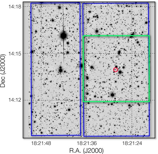
Field of view of OSIRIS. The background image was obtained by stacking all exposures of our programme. The unvignetted footprints of CCD1 (left) and CCD2 (right) are indicated in blue. The 4 arcmin × 4 arcmin area of CCD2 used for astrometry is delineated in green and centred on the target 2M1821+14 (encircled).
Table 1 summarizes the observations, including the epoch No., the mean date of the epoch exposures, the average airmass, the average FWHM measured for star images, and indicates whether the epoch was used to produce the final results. One epoch has insufficient image quality and for three epochs the target was positioned at the CCD2 edge. In two more epochs, the target was not centred sufficiently well in CCD2 and these images were not used either in the final reduction (see Section 3.2.4). The results were thus obtained with the data of 11 epochs.
Observation record for OSIRIS/GTC imaging of 2M1821+14 with the Sloan i′ filter.
| No. | Mean date | Nf | Δt | Airmass | FWHM | Used | Comment/Program |
|---|---|---|---|---|---|---|---|
| (ut) | (h) | (arcsec) | |||||
| 1 | 2013-05-08T03:55:25 | 29 | 0.88 | 1.04 | 0.93 | No | Insufficient image quality |
| 2 | 2013-05-20T01:30:47 | 26 | 0.92 | 1.20 | 0.79 | Yes | GTC37-13A |
| 3 | 2013-06-03T04:32:46 | 25 | 0.84 | 1.14 | 0.65 | Yes | GTC37-13A |
| 4 | 2013-06-05T03:25:29 | 24 | 0.84 | 1.05 | 0.92 | Yes | GTC37-13A |
| 5 | 2013-07-04T04:39:58 | 25 | 0.77 | 1.81 | 0.72 | Yes | GTC37-13A |
| 6 | 2013-07-05T02:45:32 | 27 | 0.84 | 1.19 | 0.63 | Yes | GTC37-13A |
| 7 | 2013-07-12T00:35:07 | 27 | 1.02 | 1.04 | 0.72 | No | Pointing off by ∼11 arcsec |
| 8 | 2013-07-31T23:03:41 | 55 | 1.82 | 1.04 | 0.79 | Yes | GTC37-13A |
| 9 | 2013-08-16T00:34:53 | 28 | 0.87 | 1.30 | 0.75 | No | Pointing off by ∼11 arcsec |
| 10 | 2014-07-05T23:59:15 | 24 | 1.07 | 1.05 | 0.83 | Yes | GTC11-14A |
| 11 | 2014-08-05T00:18:31 | 25 | 0.74 | 1.12 | 0.65 | Yes | GTC11-14A |
| 12 | 2014-08-31T22:10:17 | 20 | 0.57 | 1.09 | 0.92 | Yes | GTC11-14A |
| 13 | 2014-09-11T22:12:43 | 24 | 0.74 | 1.18 | 0.84 | Yes | GTC11-14A |
| 14 | 2014-10-07T21:18:03 | 26 | 0.74 | 1.35 | 0.64 | Yes | GTC11-14A |
| 15 | 2013-04-09T04:42:26 | 35 | 0.92 | 1.13 | 0.65 | No | Pointing off by ∼2 arcmin |
| 16 | 2013-05-03T03:18:21 | 29 | 0.87 | 1.11 | 0.93 | No | Pointing off by ∼2 arcmin |
| 17 | 2014-06-03T00:24:54 | 29 | 0.80 | 1.04 | 0.92 | No | Pointing off by ∼2 arcmin |
3 DATA REDUCTION AND IMAGE ANALYSIS
The raw data were bias subtracted and flat-fielded using standard methods and the calibration data provided to us by the observatory. For the astrometric analysis we used the 2000 × 2000 px central area of CCD2, which with the nominal 0.127 arcsec px scale measures ∼4 arcmin × 4 arcmin. In this area, we detected more than 800 unsaturated stars brighter than i′ = 22 and measured the positions of their photocentres. Considering that the global instrumental parameters (telescope aperture, pixel scale, FoV) of OSIRIS/GTC are similar to FORS2/VLT, we performed the astrometric reduction with the same methods that ensure the 0.1 mas astrometric precision for FORS2 data. This high astrometric precision is reached due to effective averaging of the atmospheric image motion over the large telescope aperture. The details and the latest refinements of the method are described in Lazorenko et al. (2014).
3.1 Comparison of the OSIRIS and FORS2 image profiles
One goal of this study is the investigation of the impact of the segmented mirror structure on the astrometric performance. Therefore, we analysed the shapes of star images obtained with OSIRIS and FORS2 in the central area (Section 3.1.1) and in the wings (Section 3.1.2). In Section 3.1.3, we then compare the FWHM and the intensity of the atmospheric image motion registered on both instruments.
3.1.1 PSF kernel profile
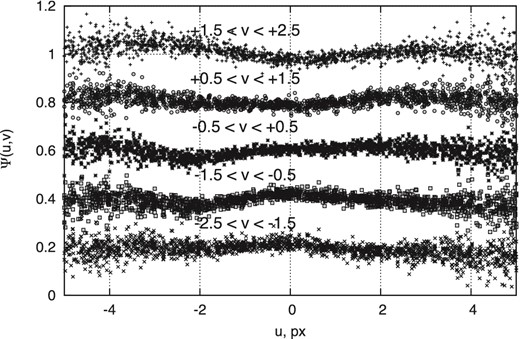
Distribution of the normalized residuals ψ(u, v) of the ‘measured–model’ pixel counts near the PSF kernel for a FORS2 example image with FWHM = 0.65 arcsec. The horizontal u-axis is aligned with the x-axis of the CCD and each sequence of data points corresponds to a slice along the v-axis.
In Fig. 3, we present the distribution of the residuals ψ(u, v) for OSIRIS separately for the left half, with x < 1000 px, and the right half (x > 1000 px) of the used area in CCD2. The size of each region is 1000 × 2000 px, comparable to the FORS2 field in the above analysis, and we chose matching seeing conditions as well. Comparison of Figs 2 and 3 shows qualitatively similar wave-like patterns of the function ψ for both telescopes.
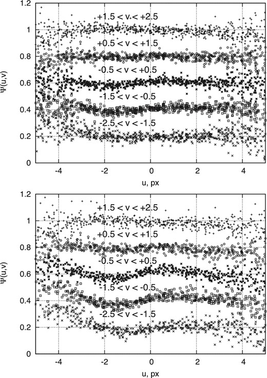
The same as Fig. 2 but for an example OSIRIS image. The two panels correspond to the two halves of CCD2 used for astrometric reduction, i.e. x < 1000 px (upper panel), and x > 1000 px (lower panel).
The random scatter of ψ(u, v) is caused mainly by photon statistics and therefore increases with |u| because of the decrease of the photoelectron counts at the periphery of the PSF. The systematic part ψsyst of ψ contains two components. The first varies between the adjacent exposures, thus indicating contribution of the atmospheric turbulence uncorrelated in time. The second component is stable during the whole frame series of one epoch and is potentially an imprint of the current optical aberrations of the telescope. An example of the fine structure of ψsyst for OSIRIS measured on 2013 July 5 is illustrated in Fig. 4.

Shape of the systematic residuals ψsyst(u, v) for a series of OSIRIS exposures obtained on 2013 July 5 with FWHM = 0.64 arcsec and visually impeccable images. The rms of ψsyst(u, v) within 2 × 2 px from the PSF centre is σ(ψ) = 0.018.
In Fig. 5, we present the values of σ(ψ), which is the rms of ψsyst within ±2 px at the kernel of the PSF. We compare that to FORS2, for which σ(ψ) was obtained for the large data set of the Sahlmann et al. (2014) survey and is represented here by a the result of a linear fit in FWHM. In comparison to FORS2, the fluctuations of ψsyst at the PSF centre are on average 50 per cent larger for OSIRIS. In both cases, the dependence of σ(ψ) on FWHM is weak and shows a comparable decreasing trend.
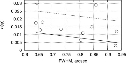
The values of σ(ψ) as a function of the FWHM in OSIRIS images for every epoch (open circles). The equivalent values for FORS2 are below the dashed line in 95 per cent cases and their mean value is indicated by the solid line.
The function ψsyst describes the fine structure of the measured star profiles (equation 3), which in general are non-symmetric and can have non-zero first derivatives of PSF(x, y) on x or y over significantly large pixel areas. In addition, the shape of the function ψsyst depends on the position in the FoV. However, we were not able to improve precision by modelling these variations because of the limited number of reference stars, thus ψsyst was assumed constant over the FoV.
The complicated structure of the PSF, in particular the one caused by optical aberrations, makes the definition of the ‘actual’ photocentre ambiguous, because it does neither coincide with the model profile centre nor with the weighted photocentre. The solution |$\bar{x}$|, |$\bar{y}$| obtained using equation (3) can therefore be displaced from the ‘actual’ photocentre. It is difficult to estimate the resulting bias of |$\bar{x}$|, |$\bar{y}$| values, but a priori we can assume that it is proportional to σ(ψ), which is the measure of irregularity of ψsyst. Fig. 5 shows that with the exception of two cases, the values of σ(ψ) for OSIRIS are slightly larger but comparable to those of FORS2. In this respect, the compound structure of the GTC main mirror does hardly affect the astrometry, at least for good images with σ(ψ) < 0.02.
3.1.2 PSF wings
Computation of photocentre positions in crowded fields or for close star pairs requires the iterative subtraction of the light from a neighbouring star image. This is realized by using a calibration PSF mask which is a pixelized accumulation of the PSF profile and represents well the actual shape of the PSF out to distances of 15 px from the centre (Lazorenko et al. 2014). The calibration image is compiled for every frame by accumulating the pixel counts in images of bright isolated stars after normalizing to some standard star brightness. Fig. 6 illustrates the calibration PSFs for two single images taken with OSIRIS and FORS2 obtained at comparable seeing with FWHM = 0.71 arcsec. For both cameras, the PSF shape is very similar, except that the outer wings of the OSIRIS image display the symmetric hexagonal pattern that reflects the shape of the primary mirror. This feature is weak and well modelled, and therefore should not degrade the astrometry.
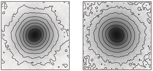
The PSF of OSIRIS (left) and FORS2 (right) shown in logarithmic scale for images taken in similar seeing conditions. The OSIRIS image replicates the hexagonal structure of the telescope pupil. Each panel measures 30 × 30 px or ∼3.8 arcsec × 3.8 arcsec.
3.1.3 Average FWHM
Both OSIRIS and FORS2 observations were acquired in service/queue mode and the distribution of FWHM therefore depends on a combination of requested seeing conditions, the program priority assigned by the time allocation committee, and the observatory science operations. For OSIRIS and FORS2, we had requested seeing ≤0.9 and ≤0.8 arcsec, respectively.
The distribution of FWHM in all used OSIRIS frames1 is shown in Fig. 7 and compared to the results of the FORS2 data (Lazorenko et al. 2014) scaled to equal number of exposures. The FWHM of OSIRIS images is 0.80 arcsec on average, which is ∼23 per cent larger than the corresponding mean FWHM of 0.65 arcsec for FORS2. The uncertainty of the photocentre positions is larger for OSIRIS by the same extent, because it is proportional to FWHM.
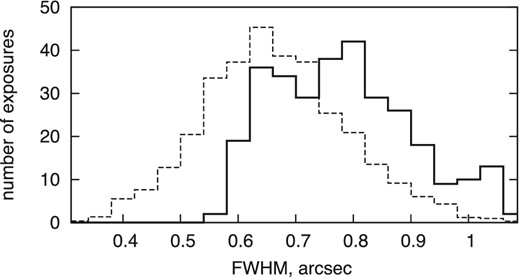
Histogram of FWHM distribution for OSIRIS images (solid) and FORS2 distribution normalized to the same number of exposures (dashed line).
3.2 Astrometric reduction
The astrometric reduction is aimed at determining the position of the target in every image relative to its location in a reference frame defined by a standard image (or its equivalent based on several images). The mapping of the reference star positions between frames is performed using basic functions which are polynomials in x,y of order 0, 1, …k/2 − 1. The even integer k is called the mode of astrometric reduction. The model accounts for the reference frame distortion caused by the telescope optics and the image motion, and it takes into account the displacements of reference stars in time due to the proper motion, parallax, and differential chromatic refraction (DCR). The system of astrometric parameters derived by this method (proper motions, offsets, chromatic parameters, and parallaxes) is constrained by a set of conditions similar to the ones imposed on the residuals of a least-squares fit via basic functions (Lazorenko et al. 2009). In particular, if the star parallaxes are randomly distributed in the FoV, the difference between the measured and true parallaxes is a constant, usually referred to as the zero-point of parallaxes. For more complicated spatial distributions of parallaxes, this difference is not flat and slowly varies with x,y.
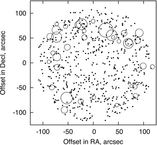
We used k values in the range of 6–16 and the corresponding radii R of reference star groups increased with k from 0.6 to 1.48 arcmin, leading to number of reference stars between 56 and 361. The geometry of the reference fields is shown in Fig. 8. Some stars are located beyond the largest reference field of 2M1821+14, because we processed not only the target itself, but also a number of nearby stars in order to detect, estimate, and mitigate space-dependent systematic errors. The reduction of these stars is performed with their respective reference fields and stars in the outer parts of Fig. 8 are also used as references to produce the catalogue presented in Section 4.6.
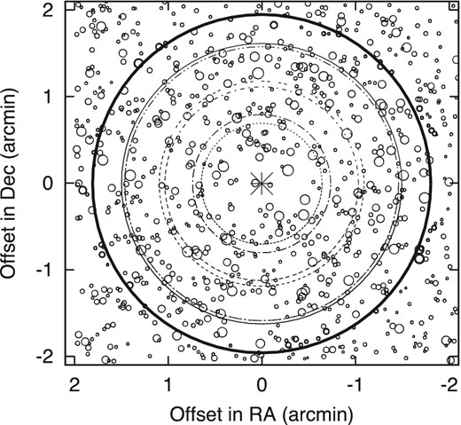
Positions of stars on the CCD2 chip of OSIRIS that were used for the astrometric reduction. 2M1821+14 is marked with an asterisk and the sizes of open circles indicate the brightnesses of reference stars. All stars are located within 2 arcmin of the target and six concentric circles with increasing radii mark the reference fields used for the reduction with k = 6–16 (Section 3.2). North is up and east is left. The outer bold circle delimits the stars included in the catalogue (Section 4.6). The shown area corresponds to the green square in Fig. 1.
3.2.1 Atmospheric image motion
3.2.2 Residuals of the astrometric model
To evaluate the quality of the astrometric reduction (and eventually to determine the astrometric parameters), we inspect the frame residuals after adjusting the linear model equation (5) to the data, which is accomplished by matrix inversion. By averaging the frame residuals of every epoch, we obtain the epoch residuals xep and yep in RA and Dec., respectively.
This reduction technique is applicable equally both to 2M1821+14 and any field star with its unique set of reference stars. Astrometric solutions for field stars are useful to test the presence of systematic errors, to derive the parallaxes of background stars, for the correction to absolute parallax, to determine the pixel scale, and for compiling the catalogue of field stars.
3.2.3 Non-standard observations
The default position of the target was chosen to be near the CCD2 centre. In the images of epoch No. 7, however, the star field was displaced by dx ≈ 90 px along the x-axis. For epoch No. 9, a similar offset occurred along both axis and the images were slightly asymmetric, although with good FWHM = 0.8 arcsec. To investigate the effect of non-standard telescope pointing on the astrometry, we ran a test reduction for 30 bright stars near the field centre. Each of these test star was processed in the same way as the target, with the epoch residuals xep, yep as output data. We used the images of these two problem epochs and also included the images of epoch No. 1, which exhibit clearly non-symmetric PSF shapes with multiple peaks and were obtained with FWHM = 0.93 arcsec, i.e. slightly above the average seeing. Usually, such images are discarded during the preliminary inspection. The computations for the total of 14 epochs were run with k = 10 only and Fig. 9 shows the scatter of the epoch residuals for these stars, which is abnormally large for the epoch Nos. 1, 7, and 9.
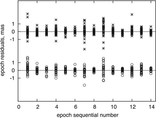
The epoch residuals xep (open circles) and yep (asterisks) for 30 bright stars as a function of epoch number. There is abnormally large scatter for epoch Nos. 1, 7, and 9.
The large scatter for the epoch No. 1 residuals is expected, because the important distortion of the PSF shape leads to effects which cannot be adequately compensated with our reduction method, thus eventually creates systematic errors in differential positions. Although the FWHM of the images in epoch Nos. 1 and No. 9 are within the tail of the distribution shown in Fig. 7, the scatter of their epoch residuals σep is increased approximately twofold, with many deviations larger than 1 mas.
The field offsets in epoch No. 7 and No. 9 have a different effect: when the geometry of the CCD is not perfect, for instance if the CCD pixel columns are curved, the field offset can affect the epoch residuals xep, yep because the local segments of CCD columns for the target and field stars can be relatively inclined, say at some angle i. If the field offset is dx, dy along the CCD axes, it results in the displacement of the CCD positions on idy and −idx along RA and Dec., respectively. Because the value of i depends on the star position in the FoV, the effect is different in RA and Dec. in terms of amplitude and sign. As a result, we expect excess random scatter of the epoch residuals in RA for the epoch No. 9, and in Dec. for the epoch No. 7 and No. 9, which is confirmed in Fig. 9.
3.2.4 Epoch residuals for nominal observations
We repeated the astrometric reduction with the eleven nominal epochs and computed the rms of the measured single-frame residuals in x and y. Both for 2M1821+14 and for a sample of bright field stars, each reduced as a target, we obtained a value of 1.05 mas. This matches the expected single-frame precision obtained from a model that accounts for the precision of the photocentre determination, the atmospheric image motion, and the reference field noise. Hence, the expected nominal precision of the epoch residuals xep, yep is σnom = 0.20 mas for a typical epoch consisting of 28 frames. This is a lower limit, which does not take into account systematic errors that affect the epoch positions but are constant during the epoch. The more complete astrometric reduction described in Lazorenko et al. (2014) allowed us to uncover the existence of systematic errors, of which some are correlated in CCD space. Their contribution to the error budget slightly increases the expected nominal epoch precision to σnom = 0.23 mas.
We compare this value to the rms of the epoch residuals xep, yep, which is σep = 0.40 mas and σep = 0.35 mas for 2M1821+14 and the bright stars, respectively. Those two values are comparable, meaning that the red and fast-moving target is measured with the same precision as field stars and it excludes the presence of orbiting companions that would introduce a measurable astrometric signature. However, the difference between the measured epoch precision of 0.35–0.40 mas and its expected value of 0.23 mas is significant and points towards unknown systematic errors.
3.2.5 Relation between σep and σ(ψ)
Finally, we ascertained that there is no correlation between σep and σ(ψ) for bright field stars. This means that if images are compact and visually symmetric, implying that the degree of deformations of the PSF kernel is σ(ψ) ≤ 0.03, they yield essentially the same results as ideal images with σ(ψ) = 0, i.e. with no excess of systematic errors in the differential positions.
4 RESULTS
To obtain the results of our astrometric study of 2M1821+14, we followed mostly the prescriptions of Sahlmann et al. (2014).
4.1 Astrometric parameters of 2M1821+14
We obtained the astrometric parameters of our target 2M1821+14 by obtaining the least-squares solution of equation (5) for the photocentre positions determined from the OSIRIS images. The solution was found using matrix inversion and takes into account the measurement uncertainties and covariances. The parameters are given in Table 2 and Figs 10 and 11 illustrate the results. The reference date TRef was chosen as the mean observation date to minimize parameter correlations, which however do not vanish because of the actual sampling of our observations, see Table 3.
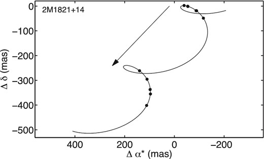
OSIRIS astrometric measurements of 2M1821+14 (circles) and the best-fitting model that includes parallax and proper motion (solid curve). The arrow indicates the proper motion direction and amplitude in 1 yr. The epoch uncertainties are comparable or smaller than the symbol size. North is up and east is left.
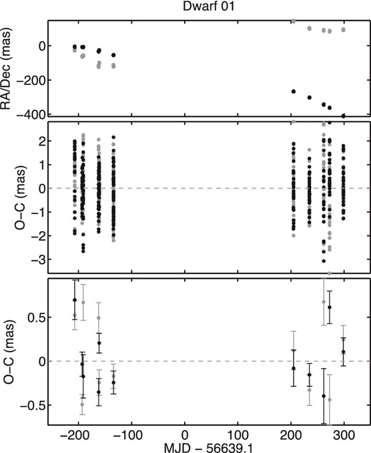
Residuals of the astrometry solution of 2M1821+14 as a function of time. The top panel shows the reduced data in RA (grey symbols) and Dec. (black symbols) and the middle panel shows the frame residuals after solving equation (5). The bottom panel shows the epoch-averaged residuals with their mean uncertainties.
Astrometric parameters of 2M1821+14. Standard uncertainties were computed from the parameter variances that correspond to the diagonal of the problem's inverse matrix and rescaled to take into account the residual dispersion.
| Δα⋆ | (mas) | 27.84 ± 0.09 |
| Δδ | (mas) | −190.36 ± 0.12 |
| ϖ | (mas) | 106.15 ± 0.18 |
| |$\mu _{\alpha ^\star }$| | (mas yr−1) | 230.27 ± 0.16 |
| μδ | (mas yr−1) | −241.49 ± 0.12 |
| ρ | (mas) | 22.08 ± 0.13 |
| Derived and additional parameters | ||
| TRef | (MJD) | 56639.124721 |
| Δϖ | (mas) | −0.50 ± 0.05 |
| ϖabs | (mas) | 106.65 ± 0.20 |
| Distance | (pc) | 9.38 ± 0.03 |
| Number of epochs/frames | 11/312 | |
| σep | (mas) | 0.401 |
Parameter correlation matrix.
| |$\Delta \alpha ^\star _0$| | Δδ0 | ϖ | |$\mu _{\alpha ^\star }$| | μδ | ρ | |
|---|---|---|---|---|---|---|
| |$\Delta \alpha ^\star _0$| | +1.00 | |||||
| Δδ0 | −0.04 | +1.00 | ||||
| ϖ | +0.44 | −0.77 | +1.00 | |||
| |$\mu _{\alpha ^\star }$| | +0.41 | −0.49 | +0.69 | +1.00 | ||
| μδ | +0.20 | −0.28 | +0.43 | +0.48 | +1.00 | |
| ρ | +0.39 | +0.56 | −0.27 | −0.11 | −0.13 | +1.00 |
Because the astrometric reference stars are not located at infinity, a correction has to be applied to the relative parallax to convert it into an absolute parallax that can yield the distance. As in Sahlmann et al. (2014), we use the Galaxy model of Robin et al. (2003) to obtain a large sample of pseudo-stars in the region around 2M1821+14. The comparison between the model parallaxes and the measured relative parallaxes of stars covering the same magnitude range yields an average offset, which is the parallax correction. Using Nstars = 450 reference stars, we obtained a parallax correction of Δϖgalax = −0.50 mas with an rms value of σgalax = 1.10 mas. The absolute parallax is ϖabs = ϖ − Δϖgalax and its uncertainty was computed by adding |$\sigma _\mathrm{galax}/\sqrt{N_\mathrm{stars}}$| in quadrature to the relative parallax uncertainty. Fig. 12 shows the magnitudes on pseudo- and reference stars, demonstrating a good match of their distributions.
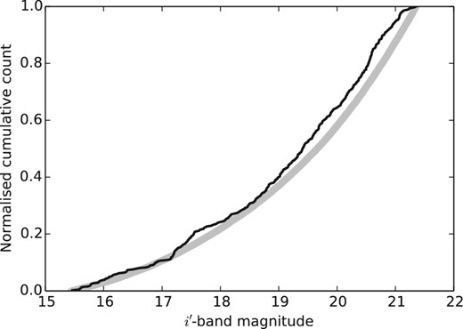
Using a Galaxy model to determine the parallax correction. Cumulative distribution of magnitudes for the used reference stars of 2M1821+14. The model and measured data are shown in grey and black, respectively.
In principle, a similar procedure should be applied to correct from relative to absolute proper motion. We refrain from doing so, because proper motion is a less critical parameter in the following analyses and the correction will be small. Our proper motions agree with the values derived by Gagné et al. (2014), however we determined them with ∼50 times smaller uncertainties. In the future, the results of ESA's Gaia mission will make it possible to determine model-independent parallax and proper motion corrections, because Gaia will obtain accurate astrometry for many of the reference stars used here.
The resulting distance of 9.38 ± 0.03 pc agrees with the spectrophotometric estimate of ∼10 pc of Looper et al. (2008). Fig. 13 shows the K-band absolute magnitude of 2M1821+14, which appears comparable to other field objects with measured precision parallaxes. This suggests that the metallicity of 2M1821+14 does not differ significantly from that of the field, and we will therefore assume that is has solar metallicity.
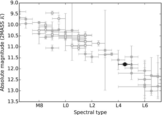
Absolute magnitude in the 2MASS K band as a function of spectral type for M6–L7 dwarfs in the data base of ultracool parallaxes (filled grey symbols; Dupuy & Liu 2012), for the FORS2 survey sample (open grey symbols; Sahlmann et al. 2014), and for 2M1821+14 with a spectral type of L4.5 (black circle).
4.2 Estimating the age of 2M1821+14
2M1821+14 was identified as a potentially young member of the field population that shows signs of low surface gravity (Looper et al. 2008; Gagné et al. 2014; Yang et al. 2015). The mid-L spectral type combined with the clearly detected lithium absorption at 670.8 nm in the optical spectrum (Looper et al. 2008) implies that its mass has to be smaller than about 0.06 M⊙ (Magazzù, Martín & Rebolo 1993). We thus assume a preliminary upper limit of ∼1 Gyr for the age of 2M1821+14, which we refine in the following.
Using the radial velocity of 9.8 ± 0.16 km s−1 (Blake et al. 2010) and the proper motions and absolute parallax of this paper, we derived the U, V, and W heliocentric velocity components in the directions of the Galactic centre, Galactic rotation, and North Galactic pole, respectively, with the formulation provided by Johnson & Soderblom (1987). We used the right-handed system and the solar motion is not subtracted from our calculations. The uncertainties associated with each space velocity component are obtained from the quoted parallax, proper motion (with 1 mas yr−1 uncertainties to account for the unknown but small offset to their absolute values), and radial velocity uncertainties after the prescriptions of Johnson & Soderblom (1987). For 2M1821+14 we find U = 12.91 ± 0.12, V = 4.62 ± 0.11, and W = −11.30 ± 0.06 km s−1. These values indicate a young kinematic age, which agrees with the results by Gagné et al. (2014). According to Eggen (1990) and Leggett (1992), these Galactic velocities are typical of the young–old disc. Although the Galactic velocities of 2M1821+14 do not fall within the 1σ ellipsoids of known young stellar moving groups (e.g. Zuckerman & Song 2004; Torres et al. 2008; Zuckerman et al. 2011) in UVW diagrams, they are relatively close to the Ursa Major moving group (see Fig. 14), which has an estimated age of 300–500 Myr.
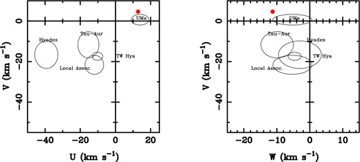
UVW velocities of 2M1821+14 (red dot) and the 1σ ellipsoids of different young moving groups. The uncertainties for 2M1821+14 have a size similar to the symbol.
With the spectroscopic rotational velocity of vsin i = 28.85 ± 0.16 km s−1 determined by Blake et al. (2010) and the photometric periodicity of 4.2 ± 0.1 h measured by Metchev et al. (2015) that is ascribed to rotation, we can calculate the minimum radius of Rsin i = 0.100 ± 0.003 R⊙. This implies that the true radius of 2M1821+14 is 0.10 R⊙ or larger. By comparison with the Lyon group's theoretical evolutionary substellar models, it is also inferred that the age of this source is younger than 1 Gyr, see Fig. 15. For an angle of the rotation axis near 90|$\deg$|, the age of 2M1821+14 would be close to 700 Myr.

A tentative lower age limit can be derived from comparison with the location of Pleiades (∼120 Myr) and field objects in colour–magnitude diagrams, of which one is shown in Fig. 16. 2M1821+14 appears closer to the field than to the Pleiades and it is not as red and luminous as Pleiades members of similar spectral type. Therefore, the most likely age of 2M1821+14 lies in the range of 120–700 Myr and we adopt a value of 500 Myr.
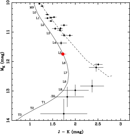
Colour–magnitude diagram showing 2M1821+14 (red large circle) and Pleiades members (black small dots) from Bihain et al. (2010) and Zapatero Osorio et al. (2014). The solid line shows the field (according to Stephens et al. 2009) and the dashed line represents the 120 Myr isochrone following Zapatero Osorio et al. (2014).
4.3 Mass estimate of 2M1821+14
To continue interpreting our results, in particular to derive limits on the masses of potential companions, a mass estimate of 2M1821+14 is required. Because we rely on photometry, the estimated masses of ultracool dwarfs are tightly linked to their ages. Assuming an age range of 120–700 Myr, we used a method that relies on an estimation of the bolometric luminosity. We converted 2mass magnitudes to the mko system using updated colour transformations (Carpenter 2001)3 and bolometric corrections (Liu, Dupuy & Leggett 2010) to obtain the luminosity. The corresponding mass at a given age was found by interpolating the DUSTY models (Chabrier et al. 2000). Differences between J,H,K bands are negligible, and we used their average. The resulting masses are listed in Table 4 and include the uncertainties in apparent magnitude, parallax, and spectral type (assumed to be L4.5 ± 1). Those formal uncertainties are sometimes smaller than the model uncertainties, which we assume to be 10 per cent on the derived masses.
Mass estimates for 2M1821+14 with theoretical formal uncertainties.
| Age | Mass |
|---|---|
| (Gyr) | (M⊙) |
| 0.12 | 0.024 ± 0.004 |
| 0.50 | 0.049 ± 0.001 |
| 1.00 | 0.063 ± 0.001 |
| Age | Mass |
|---|---|
| (Gyr) | (M⊙) |
| 0.12 | 0.024 ± 0.004 |
| 0.50 | 0.049 ± 0.001 |
| 1.00 | 0.063 ± 0.001 |
We see that for ages younger than 1 Gyr, 2M1821+14 has a mass smaller than the lithium-burning mass limit, which is consistent with the presence of Li i absorption in its optical spectrum (Looper et al. 2008). According to this method the mass of 2M1821+14 would be |$0.049^{+0.014}_{-0.025}\,\text{M}_{{\odot }}$| for an age of |$500^{+200}_{-380}$| Myr.
4.4 Planet detection limits
One of the goals of this study is to evaluate the potential of OSIRIS astrometry for planet discovery. Already with the data collected here, we are able to exclude the presence of companions to 2M1821+14 that have orbital periods comparable to the timespan of OSIRIS observations, i.e. ∼500 d. We estimated the companion detection limits following the procedure described in Sahlmann et al. (2014). This procedure assumes that the light contribution of the companion to the photocentre motion is negligible, which may not be the case for young and high mass-ratio systems (cf. Sahlmann et al. 2015).
Fig. 17 shows the maximum mass of any putative companion to 2M1821+14 as a function of its orbital period and projected physical separation. In particular, for orbital periods between ∼50 and ∼1000 d (∼0.1–0.7 au), the OSIRIS/GTC data exclude at 3σ confidence the presence of any companion down to a mass ratio of 0.1, corresponding to a planet with a mass of about 5 Jupiter masses (MJ). The low mass and nearby distance of 2M1821+14 are favourable to push the detection limit to small companion masses, despite the residual dispersion of 0.4 mas that is larger than the average value of 0.12 mas achieved for FORS2.
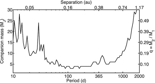
Companion detection limits for 2M1821+14 as a function of orbital period (bottom label) and relative primary–secondary separation (top label, computed for a 5 MJ companion around a 0.049 M⊙ primary). The right label indicates the mass ratio q. The maximum companion mass compatible with the measurements is shown, i.e. companions on and above the curve are excluded by the data at 3σ confidence.
4.5 Optical variability of 2M1821+14
We performed relative photometry of 2M1821+14 with the OSIRIS data using the method of Sahlmann et al. (2014), which is based on brightness measurements of 2M1821+14 and dozens of field stars in each of the eleven astrometric epochs. We used different sets of comparison stars (between 10 and 60) and obtained very similar results. The photometric variation of 2M1821+14 is 12 mmag rms in the Sloan i′ band as shown in Fig. 18. This is higher than the typical variability for reference stars that have values of 1–5 mmag with an average of 3 mmag rms, a value that represents the uncertainty of the method. We used the reference star photometry to investigate correlations with airmass (which varied between 1.0 and 2.0) or sky conditions but found none. Our observations therefore suggest that 2M1821+14 shows optical variability at >10 mmag level on time-scales of weeks to years.
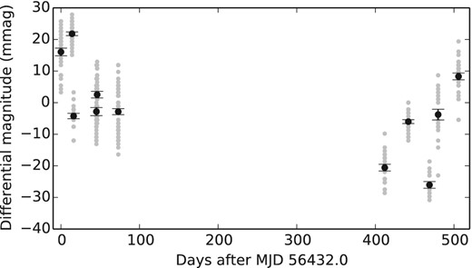
Differential magnitude variation of 2M1821+14 in i′ band as a function of time. Grey symbols correspond to measurements in individual OSIRIS frames, whereas black circles show the epoch averages with uncertainties given as error of the mean.
2M1821+14 was also monitored by Koen (2013), who did not detect significant optical variability, and a near-infrared spectral variability study was performed by Yang et al. (2015). Finally, Metchev et al. (2015) detected infrared variability with a period of 4.2 ± 0.1 h. We examined our OSIRIS photometry for periodic variations at similar time-scales using a periodogram analysis, but did not find a significant signal. This may be explained by an amplitude that is much smaller in the optical than at 3.6/4.5 μm or by the sampling of our data, which consists of eleven epochs with ∼55 min duration each, separated by several days or weeks. In addition, the 4.2 h photometric signal detected in the 10 h continuous timeseries of Metchev et al. (2015) may not be phase-coherent over time-scales of years, reducing the probability of detecting it with our OSIRIS photometry.
4.6 Catalogue of field stars
We supplement this study with the astrometric parameters of the 587 stars with magnitudes i′ = 15.5–22 that were used as astrometric references in the field of 2M1821+14, i.e. that are located within 2 arcmin of the target. We computed their parameters with the reduction mode k = 10. The typical precision of their parallaxes varies from 0.15 to 2.5 mas depending on brightness and the uncertainty of proper motions ranges from 0.1 to 3 mas yr−1. There are no stars with proper motions larger than ±10 mas yr−1.
Fig. 19 presents the absolute parallaxes ϖa as a function of magnitude and shows that the majority of stars is at least 200 pc distant. Most measurements are within the ±3 σϖ uncertainty limits expected for stars located at infinite distance.
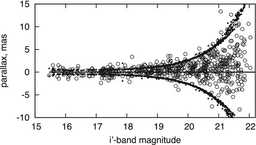
The measured absolute parallaxes of field stars (open circles) which lie mostly within statistical +3σ upper and −3σ lower limits indicated by solid circles for stars at infinite distance. Absolute parallaxes were obtained from the relative parallaxes given in the catalogue and the 0.50 mas correction.
However, about 30 stars have negative parallaxes beyond the −3 σϖ level and as shown in Fig. 20 those are concentrated in a few isolated areas of the FoV periphery. Whereas underestimated parallax uncertainties are unlikely to lead to this space-correlated pattern, a slow change of the zero-point of parallaxes across the FoV could be the cause. As commented in Section 3.2, the parallaxes are determined on the basis of polynomial functions in the spatial coordinates x,y. Therefore, if the spatial distribution of parallaxes is strongly inhomogeneous, the systematic difference between ϖa and the real parallaxes is not flat and can slowly change with x,y, creating local zones with deviating parallaxes. In Fig. 20, we can see such areas where parallaxes of bright stars are excessively negative. The size of these areas is small and no outlying parallaxes are found in other parts of the FoV, in particular in the field centre. Therefore, our estimate of the parallax of 2M1821+14 is not expected to be biased. In addition, we verified that limiting the reference star sample for the parallax correction (Section 4.1) to stars within <1 arcmin, i.e. excluding the parallax outliers, yields an essentially identical result Δϖ = −0.44 ± 0.10.
On-sky position of all catalogue stars (black dots) and stars which measured absolute parallax is below −3 σϖ (open circles). The circle size is proportional to the ratio −ϖa/σϖ.
The relative parallaxes and proper motions of reference stars are available at the Centre de Données astronomiques de Strasbourg (CDS) as a catalogue which contains RA and Dec. in the ICRF. Transformation to the ICRF system was performed using the USNO-B catalogue (Monet et al. 2003). There are 45 stars in the 2M1821+14 field for which we obtained precise astrometry with OSIRIS and that were included in USNO-B. We mapped their positions using quadratic and cubic polynomials with a resulting rms difference of 0.17 arcsec, which allowed us to find the absolute positions with an uncertainty of ∼ 0.04–0.2 arcsec, propagated from the USNO-B data. This exceeds the precision of the original relative positions by a factor ∼1000. We plan to update the absolute positions using the Gaia astrometric catalogues, when they become available. The i′-band magnitudes will have to be updated as well, because none of the reference stars has published i′-band photometry, necessary for conversion from the instrumental to standard magnitudes. The only reference is the Cousins IC = 17.0 ± 0.2 estimate given by Koen (2013) for 2M1821+14, which we used for zero-point determination. We neglected the difference between the Cousins IC and Sloan i′ systems, which is small in comparison to the random error of 0.2 mag of the Koen (2013) measurement. Consequently, although the zero-point is from a IC magnitude, our photometry relates to Sloan i′.
The catalogue also contains the quality flag χ2 for each star, which is the average ratio of |$x_{\rm ep}^2$| and |$y_{\rm ep}^2$| to the model variance. For a random sample following a normal distribution, we expect to register χ2 ≈ 1 on average, but the measured data in Fig. 21 exhibit a large scatter and an increase at the bright end. The observed large deviations χ2 ≥ 10 were found to correspond to blended images. Excluding those cases, we found a linear dependence of χ2 on i′, which approaches unity for faint stars and a value of 2.6 at the magnitude of 2M1821+14. The value χ2 = 4.5 obtained for 2M1821+14 lies in the tail of the χ2 distribution for field stars. A smaller excess in χ2, usually within 1.1–1.5 and not related to underestimated uncertainties, was already noticed for FORS2 observations (Lazorenko et al. 2014). The OSIRIS data do not allow us to conclude on the nature of the systematic excess in χ2 and we attribute it to a systematic error that remains to be characterized.
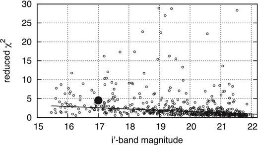
Distribution of the reduced χ2 values as a function of magnitude for field stars (open circles) and a linear approximation (solid line). The solid circle marks 2M1821+14 with χ2 = 4.5.
Table 5 shows the content of the catalogue, which contains the sequential star number Nr in the field, the i′-band magnitude and its internal precision |$\sigma _{i^{\prime }}$|, RA and Dec. for the equinox and epoch J2000.0 with their uncertainties, the relative proper motion |$\mu _{\alpha ^\star }$|,cos δ and μδ per Julian year and uncertainties, the relative parallax ϖ with uncertainty σϖ, and the DCR parameter ρ. The mean epoch of observations is given by |$\bar{T}$| in Julian years since J2000, and the χ2-value for the epoch residuals flags the quality of the fit.
Excerpt of the astrometric catalogue. The full table is available online and at the CDS.
| Nr | i′ | |$\sigma _{i^{\prime }}$| | RA | σα | Dec. | σδ | |$\mu _{\alpha ^\star }$| | |$\sigma _{\mu _{\alpha ^\star }}$| | μδ | |$\sigma _{\mu _{\delta }}$| | ρ | σρ | ϖ | σϖ | |$\bar{T}$| | χ2 |
|---|---|---|---|---|---|---|---|---|---|---|---|---|---|---|---|---|
| (mag) | (mag) | (deg) | (arcsec) | (|$\deg$|) | (arcsec) | (mas | (mas | (mas | (mas | (mas) | (mas) | (mas) | (mas) | (yr) | ||
| yr−1) | yr−1) | yr−1) | yr−1) | |||||||||||||
| 41 | 20.409 | 0.006 | 275.3611854 | 0.639 | 14.2014463 | 0.537 | −0.9 | 1.16 | 0.39 | 0.91 | 3.28 | 0.94 | 3.53 | 1.21 | 14.0043 | 0.63 |
| 51 | 20.061 | 0.005 | 275.3601554 | 0.604 | 14.2020711 | 0.506 | −0.26 | 0.85 | 3.12 | 0.67 | −4.46 | 0.71 | 0.63 | 0.92 | 14.0043 | 0.81 |
| 54 | 20.597 | 0.006 | 275.3638648 | 0.579 | 14.2023064 | 0.484 | −3.97 | 1.36 | −4.53 | 1.06 | −4.34 | 1.17 | −1.07 | 1.44 | 14.0043 | 2.14 |
| 58 | 19.437 | 0.004 | 275.3652450 | 0.561 | 14.2025570 | 0.468 | 5.1 | 0.51 | −3.38 | 0.39 | 6.82 | 0.42 | 1.92 | 0.54 | 14.0043 | 3.94 |
| 60 | 18.418 | 0.002 | 275.3620758 | 0.567 | 14.2025922 | 0.473 | 1.63 | 0.25 | 1.25 | 0.19 | −0.49 | 0.2 | −0.74 | 0.27 | 14.0043 | 2.96 |
4.7 OSIRIS pixel scale
The conversion from CCD pixel space to on-sky angular space was performed based on the USNO-B positions. This allowed us to derive a pixel scale of 129.11 ± 0.18 mas px−1, which differs from the value of 127 mas px−1 given in the OSIRIS documentation (http://www.gtc.iac.es/instruments/osiris/osiris.php). This difference could be caused by the thermal change of the telescope focal length and we emphasize that our updated scale is valid at the target position only. The difference between the pixel scales we determined along x- and y-axes is 0.16 ± 0.25 mas px−1, thus not significant.
5 CONCLUSIONS
We obtained multi-epoch imaging observations of the L4.5 dwarf 2M1821+14 with OSIRIS/GTC in i′ band spanning 17 months and applied methods developed for FORS2/VLT to measure its astrometric motion relative to field stars. We performed a first analysis of the astrometric performance of OSIRIS in comparison with the well-studied properties of FORS2. The segmented structure of GTC's main mirror produces a slightly more complicated PSF shape, which however does not significantly affect the astrometry.
With OSIRIS we achieved a single-frame astrometric precision of 1.0 mas for a well-exposed star, an exposure time of 45 s, the reference star density of the 2M1821+14 field, and the average FWHM of 0.80 arcsec. The expected precision for one epoch consisting of 28 single frames is then 0.23 mas. However, the measured rms dispersion of epoch residuals is σep = 0.35–0.40 mas, thus significantly larger for reasons not yet fully understood. With additional OSIRIS data taken with a similar observation strategy, we hope to develop optimised reduction methods to reach the 0.23 mas accuracy limit set by the image motion, seeing, and the reference frame noise.
In comparison to typical FORS2 observation at VLT presented in Lazorenko et al. (2014) and Sahlmann et al. (2014), we have measured a 23 per cent larger FWHM and a factor of 2.2 larger image motion for the 2M1821+14 observations with OSIRIS. These two factors explain why the photocentre precision is 0.23 mas for OSIRIS compared to 0.12 mas for FORS2. The larger image motion of OSIRIS can be explained by larger atmospheric turbulence at high altitudes, by instabilities of the GTC and its optics, or by a combination thereof. GTC observations in better atmospheric conditions than met here are expected to yield better astrometric precision.
Using the 11 observation epochs, we determined a trigonometric distance of 9.38 ± 0.03 pc to the L4.5 dwarf 2M1821+14, which represents the first astrophysical application of precision astrometry with OSIRIS/GTC. This is also the first parallax determination for 2M1821+14, which establishes it as a member of the 10 pc sample. We measured the proper motion of 2M1821+14 with high precision and the resulting galactic kinematics are consistent with the suspected youth of this source. The data exclude the presence of binary or planetary companions with masses as low as 5 MJ and periods of 50–1000 d (≈0.1–0.7 au), which illustrates the potential of OSIRIS astrometry for exoplanet and binary search and orbit characterization.
In summary, we demonstrated that the OSIRIS camera of the GTC is capable of measuring differential positions with an accuracy of 0.35–0.40 mas over a timespan of 1.4 yr. We thus established OSIRIS as an instrument suitable for high-precision astrometry for faint optical sources located in the Northern hemisphere. This study is relevant for the development of astrometric programs with extremely large optical telescopes like the E-ELT and TMT, which also employ segmented primary mirrors. The precision level of 0.1–0.3 mas explored here is however one order of magnitude larger than what can be expected for optical telescopes with apertures of 30–40 m.
JS is supported by an ESA Research Fellowship in Space Science. This research made use of the data bases at the Centre de Données astronomiques de Strasbourg (http://cds.u-strasbg.fr); of NASA's Astrophysics Data System Service (http://adsabs.harvard.edu/abstract_service.html); of the paper repositories at arXiv; of the M, L, T, and Y dwarf compendium housed at DwarfArchives.org; and of Astropy, a community-developed core python package for Astronomy (Astropy Collaboration et al. 2013).
Based on observations made with the Gran Telescopio Canarias (GTC), installed at the Spanish Observatorio del Roque de los Muchachos of the Instituto de Astrofísica de Canarias, in the island of La Palma (Program IDs GTC37-13A and GTC11-14A).
This sample does not include the frame series excluded because of poor image quality or telescope pointing.
We use the notation α⋆ = αcos δ throughout the text.
REFERENCES
Supporting Information
Additional Supporting Information may be found in the online version of this article:
Table 5. Excerpt of the astrometric catalogue.
Please note: Oxford University Press is not responsible for the content or functionality of any supporting materials supplied by the authors. Any queries (other than missing material) should be directed to the corresponding author for the article.
