Type Ia supernovae from violent mergers of carbon–oxygen white dwarfs: polarization signatures Free

Abstract

1 INTRODUCTION

Despite much effort, we still lack a comprehensive picture of the progenitor systems and explosion mechanisms of Type Ia supernovae (SNe Ia). The general consensus is that SNe Ia are thermonuclear explosions of carbon–oxygen white dwarf stars in close binary systems (see e.g. Röpke et al. 2011; Hillebrandt et al. 2013, for reviews), but the exact circumstances leading to these events are unclear.

In the so-called single-degenerate scenario (Whelan & Iben 1973), a carbon–oxygen white dwarf accretes material from a non-degenerate companion and explodes when it approaches the Chandrasekhar limit. However, alternative possibilities have been proposed. Among them, one promising mechanism involves the merger of two carbon–oxygen white dwarfs (Iben & Tutukov 1984; Webbink 1984). Although the white dwarf merger is able to naturally explain many observed properties of SNe Ia (see e.g. Maoz, Mannucci & Nelemans 2014, for a review), it is unclear whether the explosion is triggered during the dynamical merger phase or later on. In the latter scenario, the primary star is believed to explode inside the merger remnant left behind by the complete disruption of the lighter star (Benz et al. 1990; Van Kerkwijk, Chang & Justham 2010; Shen et al. 2012; Zhu et al. 2013; Dan et al. 2014; Raskin et al. 2014; Kashyap et al. 2015). In the former, instead, the violent nature of the accretion process is thought to create conditions for an explosive carbon ignition during the merger (Guillochon et al. 2010; Pakmor et al. 2010, 2012, 2013; Moll et al. 2014).

Radiative transfer calculations for violent merger models have shown that the match with spectra and light curves of normal SNe Ia is reasonable for relatively massive white dwarf pairs (Pakmor et al. 2012; Röpke et al. 2012; Moll et al. 2014). It has also been shown that, for less massive white dwarfs, the model might account for certain sub-luminous SNe Ia like PTF10ops or SN 2010lp (Kromer et al. 2013). However, violent merger models have been called into question – particularly for normal SNe Ia – because they produce highly asymmetric ejecta that appear to be in contrast with the low level of polarization typically observed (see Wang & Wheeler 2008, for a review). For instance, Maund et al. (2013) recently obtained high-quality data for SN 2012fr at four different epochs and found that the polarization was consistently below 0.1 per cent. They suggested that such low level of polarization was inconsistent with the asymmetric ⁵⁶Ni distribution predicted by the violent merger model of Pakmor et al. (2012). Comparing predictions of hydrodynamic simulations with observations, however, is not trivial and requires that polarization calculations are performed for the specific ejecta morphology.

Here we present an initial spectropolarimetric investigation of the violent merger scenario. Specifically, we focus on the model of Pakmor et al. (2012), which has been used as a benchmark for the violent merger scenario in several previous studies (e.g. Röpke et al. 2012; Summa et al. 2013; Scalzo et al. 2014; Seitenzahl et al. 2015). We note, however, that the conclusions drawn in this paper may not necessarily be valid in other merger models for which the ejecta morphologies can be substantially different (e.g. Pakmor et al. 2010, 2013; Kromer et al. 2013; Moll et al. 2014).

In Section 2 we give a brief description of the explosion model of Pakmor et al. (2012), while in Section 3 we discuss the details of the radiative transfer calculations. We present synthetic observables for the violent merger model in Section 4, together with comparisons to spectropolarimetric data of normal SNe Ia. Finally, we discuss our results and draw conclusions in Section 5.

2 MODEL

The binary system studied by Pakmor et al. (2012) comprises two white dwarfs with masses of 1.1 and 0.9 M_⊙ and initial compositions of 47.5 per cent ¹²C, 50 per cent ¹⁶O and 2.5 per cent ²²Ne. In this model, a detonation is assumed to be ignited following the disruption of the secondary star, when material on the surface of the primary reaches sufficiently high densities and temperatures (Seitenzahl et al. 2009). The detonation starts to propagate and the energy release from nuclear burning eventually leads to a thermonuclear explosion that unbinds the merging object.

Pakmor et al. (2012) followed the evolution of the system until 100 s after ignition, by which time the ejecta have entered the homologous expansion phase. During the explosion, 0.7 M_⊙ of iron group elements (IGEs) is synthesized, of which the most abundant isotope (0.61 M_⊙) is radioactive ⁵⁶Ni. In addition, 0.5 M_⊙ of intermediate-mass elements (IMEs) and 0.5 M_⊙ of oxygen are produced, with 0.15 M_⊙ of carbon left unburned in low-density regions.

Fig. 1 shows two slices through the composition of the ejecta – mapped to a 200³ Cartesian grid – 100 s after explosion. The ejecta structure is highly aspherical, owing to the asymmetry of the merging object at the time of ignition. However, the ejecta are fairly symmetric about the x–y plane in which the inspiral and the merger phases take place before the explosion (i.e. the orbital plane). A distinctive feature is given by the cavity in the IGE distribution. As described by Pakmor et al. (2012), this feature is created as a direct consequence of the different velocities with which the detonation flame propagates inside the merged object. Given that the propagation is faster through high-density regions, the primary star burns first and its ashes have expanded considerably by the time the secondary is completely burned. Therefore, the inner parts of the ejecta are dominated by the ashes of the secondary and do not contain IGEs.

Figure 1.

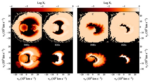
Composition of the ejecta for the model of Pakmor et al. (2012) 100 s after explosion. The mass fractions of carbon, oxygen, IMEs (from silicon to calcium) and IGEs are mapped to a 200³ grid and shown for two slices through the x–z plane (left-hand panels) and the equatorial x–y plane (right-hand panels).

Open in new tabDownload slide

3 RADIATIVE TRANSFER CALCULATIONS

Although radiative transfer calculations for the model introduced in Section 2 have already been presented in Pakmor et al. (2012), here we report new simulations that include polarization. As in the previous study, we remap the model to a 50³ Cartesian grid and perform calculations by using our 3D Monte Carlo radiative transfer code Applied Radiative Transfer In Supernovae (artis; Sim 2007; Kromer & Sim 2009). Assuming local thermodynamic equilibrium for the first 10 time-steps (t < 2.95 d) and a grey approximation for optically thick cells (Kromer & Sim 2009), we follow the propagation of N_q Monte Carlo quanta over 111 logarithmic time-steps from 2 to 120 d after explosion. While Pakmor et al. (2012) used N_q = 1 × 10⁸ and restricted to a simplified atomic data set (‘cd23_gf-5’, see table 1 of Kromer & Sim 2009), here we utilize N_q = 2 × 10⁸ and the more extended atomic data set described by Gall et al. (2012).

Synthetic observables presented in this paper are extracted exploiting a method recently implemented in artis (Bulla, Sim & Kromer 2015). In this technique (event-based technique, EBT), viewing-angle observables are calculated by summing contributions from virtual packets created at each Monte Carlo quanta interaction point and forced to escape to a selected observer orientation. Using the EBT, here we compute intensity and polarization spectra for virtual packets escaping between 10 and 30 d after explosion with rest-frame wavelength in the range 3500–10 000 Å. Aiming to investigate the impact of aspherical ejecta on the observables, we select five different observer orientations (see Fig. 2). Guided by the findings of Pakmor et al. (2012), we first choose the two orientations for which the model is faintest, |$\boldsymbol {n}_1=(0,0,1)$|⁠, and brightest, |$\boldsymbol {n}_2=(0,1,0)$|⁠. We then place two observers with orientations that are aligned with the cavity in the IGE distribution that is due to material from the secondary (see Section 2): one facing the cavity, |$\boldsymbol {n}_3=(-{}^{1}/{\scriptsize\sqrt{2}},-{}^{1}/{\scriptsize\sqrt{2}},0)$|⁠, and one at the opposite side, |$\boldsymbol {n}_4=({}^{1}/{\scriptsize\sqrt{2}},{}^{1}/{\scriptsize\sqrt{2}},0)$|⁠. Finally, we select a viewing angle away from the orbital plane and the polar axis, specifically |$\boldsymbol {n}_5=({}^{1}/{\scriptsize 2},{}^{1}/{\scriptsize 2},{}^{1}/{\scriptsize\sqrt{2}})$|⁠. Given that polarization spectra are typically noisier in the red where the flux is lower, this simulation has been supplemented by an additional calculation with N = 1 × 10⁸ and for virtual packets with emergent rest-frame wavelength between 6300 and 10 000 Å.

Figure 2.

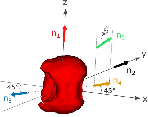
Sketch depicting the orientations of the five observers selected in this work with respect to the ⁵⁶Ni distribution. Viewing angles |$\boldsymbol {n}_2$|⁠, |$\boldsymbol {n}_3$| and |$\boldsymbol {n}_4$| are in the equatorial plane, with |$\boldsymbol {n}_3$| facing the cavity created by the presence of the secondary star (see the text).

Open in new tabDownload slide

In addition, we also carried out a simulation with N_q = 5 × 10⁷ Monte Carlo quanta and with polarization spectra extracted for an additional 30 viewing angles. Owing to its lower signal-to-noise (a factor of 4 fewer packets than in the previous simulation), the purpose of this calculation is not to study spectral features in details but rather to map out the range of polarization covered by the model.

4 SYNTHETIC OBSERVABLES

In the following, we present synthetic observables extracted with the EBT for the explosion model introduced in Section 2. In Section 4.1 we show flux and polarization spectra around maximum light for the five observer orientations selected above. We study the spectral evolution in Section 4.2 and finally compare our predictions with spectropolarimetric data of normal SNe Ia in Section 4.3.

4.1 Polarization around maximum light

In Fig. 3, we report flux and polarization spectra at 21 d after explosion (around B-band maximum light) for the five orientations chosen in Section 3. As expected, we find the same strong viewing-angle dependences reported for the spectra by Pakmor et al. (2012, but see also Moll et al. 2014). Packets escaping away from the equatorial plane (along |$\boldsymbol {n}_1$| or |$\boldsymbol {n}_5$|⁠) sweep out a larger velocity range in their journey to the observer compared to those escaping in the equatorial plane (see the ejecta distribution in Fig. 1) and the corresponding spectra are therefore affected by broader features and stronger blending of lines. In addition, the projected areas of the ⁵⁶Ni along |$\boldsymbol {n}_1$| and |$\boldsymbol {n}_5$| are smaller than those along the chosen equatorial directions and this, together with the higher opacity seen by the escaping packets, translates into fainter spectra. Despite this general trend, the spectrum seen down the cavity (along |$\boldsymbol {n}_3$|⁠) is fainter than the other two equatorial viewing angles because less IGE material is located on the side near the observer. Compared to the other four orientations, the spectrum extracted along |$\boldsymbol {n}_3$| is also markedly different, in the sense that it is characterized by much weaker and less blueshifted absorption lines. The latter results were also predicted by Kasen et al. (2004) for a somewhat similar situation in which a companion star in the single-degenerate scenario carves out a hole in the ejecta of an exploding white dwarf. Unlike our model, however, Kasen et al. (2004) adopted a density profile that leads to lines of sight through the hole having a lower-than-average column density (see their fig. 1). Therefore, they predict spectra that are typically brighter when viewed through the hole, in contrast with what we see in our model.

Figure 3.

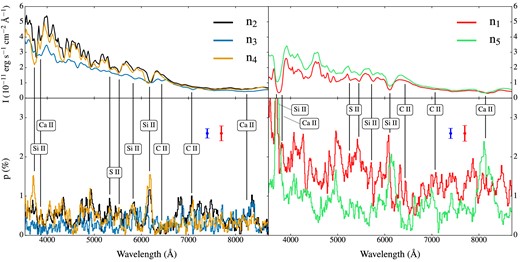
Flux and polarization spectra at 21 d after explosion for five different viewing angles (see Fig. 2). Observers in the orbital plane (black, blue and orange, left-hand panels) typically see brighter and less polarized spectra than those out of the plane (red and light green, right-hand panels). Black vertical lines and labels provide identifications between polarization peaks and some individual spectral transitions for light and intermediate-mass elements. The error bars mark the averaged Monte Carlo noise level in the polarization spectra below (blue) and above (red) 6400 Å, estimated as in Bulla et al. (2015). Polarization spectra are Savitzky–Golay filtered on a scale of 3 pixels (∼40 Å) for clarity. The model flux is given for a distance of 1 Mpc.

Open in new tabDownload slide

As expected from the asymmetric distribution of the ejecta, non-zero polarization levels are obtained for all the five chosen viewing angles. As shown in Fig. 3, we find the polarization signals to be relatively weak in the spectral range between 6400 and 7200 Å, often studied as a pseudo-continuum region that is devoid of strong line features (Patat et al. 2009). Specifically, the pseudo-continuum polarization level is modest (∼0.3 per cent) for orientations in the equatorial plane (⁠|$\boldsymbol {n}_2{\rm -}\boldsymbol {n}_4$|⁠), while higher (0.5–1 per cent) for spectra extracted along |$\boldsymbol {n}_1$| and |$\boldsymbol {n}_5$|⁠. In spite of showing weak signals in the pseudo-continuum region, however, polarization spectra for all the orientations are characterized by strong (1–2 per cent) peaks associated with blueshifted absorption troughs of spectral lines. While the identification to individual transitions is obvious for some polarization features (e.g. for Si ii and Ca ii lines), it is less clear in the blue region between 4000 and 5000 Å that is affected by stronger line blending.

Compared to the angular binning approach used by Pakmor et al. (2012), the virtual packet technique of Bulla et al. (2015) allows us to extract spectra with lower Monte Carlo noise and thus to clearly identify weak lines in the red region of the spectrum. For instance, by combining information from intensity and polarization spectra, we attribute two features in the range 6200–7300 Å to C ii λλ6580 and 7234 (see Fig. 4). While we see evidence for the C ii λ6580 feature as a notch in the emission wing of the Si ii λ6355 profile, the polarization counterpart is not visible.¹ Despite being weak and hard to see in the flux spectrum, however, the C ii λ7234 line does clearly show up in polarization with ∼1 per cent level at peak. Both these C ii lines are found at rather low velocities (v ∼ −6800 km s⁻¹) and are therefore associated with unburned carbon material in inner regions of the ejecta (see Fig. 1 and discussion in Section 5).

Figure 4.

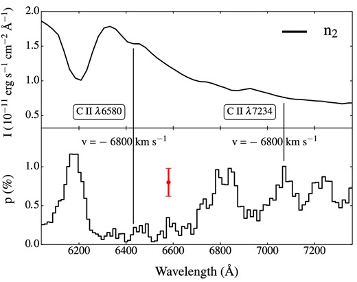
Identification of C ii λλ6580 and 7234. Flux and polarization spectra are reported at 21 d after explosion for the viewing angle |$\boldsymbol {n}_2$|⁠. Vertical lines represent a 6800 km s⁻¹ blueshift relative to the two carbon features. A red error bar marks the averaged Monte Carlo noise in the spectral range considered. Polarization spectra are Savitzky–Golay filtered on a scale of 3 pixels (∼40 Å) for clarity.

Open in new tabDownload slide

The Q/U plane provides a valuable tool for linking polarization spectral features to the ejecta structure: straight lines in this plane suggest the presence of a dominant axis in the ejecta, while deviations from straight lines (e.g. loops) reflect departures from axisymmetry. This is illustrated in Fig. 5, in which we show the Q/U plane, polarization level p (=|$\sqrt{Q^2+U^2}/I\big )$| and polarization angle χ (derived from tan 2χ = U/Q) for each of the chosen observers. As expected, the symmetry about the orbital plane results in data points distributed along a dominant axis in the Q/U planes for |$\boldsymbol {n}_2$|⁠, |$\boldsymbol {n}_3$| and |$\boldsymbol {n}_4$|⁠: the up/down symmetry causes every contribution to U from the Northern hemisphere to be cancelled by a contribution in the Southern hemisphere and the U values are therefore consistent with zero. The polarization angles derived are small which, for these specific orientations, corresponds to an electric field oscillating almost perpendicular to the equatorial plane. In contrast, Q/U planes for orientations out of the equatorial plane are characterized by loops associated with different spectral features, mainly Si ii and Ca ii. For instance, we see two distinct loops in the blue region below 4000 Å when the system is viewed pole-on (along |$\boldsymbol {n}_1$|⁠): the bluer loop is associated with the Si ii λ3859 line and shows a polarization angle comparable to that of the Si ii λ6355 feature (χ ∼ −30°); the redder loop is instead associated with the Ca H and K line and shows a polarization angle comparable to that of the Ca ii IR triplet (χ ∼ −10°).

Figure 5.

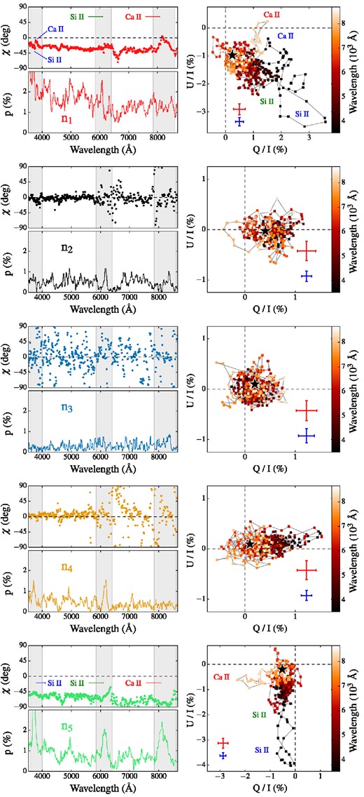
Polarization percentage p and polarization angle χ (left-hand panels), together with the corresponding Q/U planes (right-hand panels) for the spectra shown in Fig. 3. For each Q/U plot, a black star indicates the averaged polarization level in the pseudo-continuum range between 6400 and 7200 Å, while the error bars mark the averaged Monte Carlo noise level in the spectra below (blue) and above (red) 6400 Å. The Stokes parameters are Savitzky–Golay filtered on a scale of 3 pixels (∼40 Å) for clarity. For the |$\boldsymbol {n}_1$| and |$\boldsymbol {n}_5$| viewing angles, we associate individual loops or structures in the Q/U plane with specific features in the spectra.

Open in new tabDownload slide

4.1.1 Additional diagnostics

To further investigate how asymmetries in the element distribution are related to individual polarization spectral features, here we inspect the ejecta morphology of our model more closely. Polarization levels across spectral lines can be understood as the result of partial covering of the effective electron-scattering photosphere. Fig. 6 shows the intensity and polarization distributions projected on the plane perpendicular to the viewing angle |$\boldsymbol {n}_5$|⁠. The maps have been calculated selecting the emergent virtual packets between 18.5 and 23.5 d after explosion and in four different spectral regions: 6400–7200 Å (pseudo-continuum range), 3600–4000 Å (comprising the Si ii λ3859 and Ca H and K lines), 5850–6400 Å (Si ii λ6355) and 7850–8700 Å (Ca ii IR triplet). The pseudo-continuum region is almost devoid of lines and therefore more representative of the underlying electron-scattering photosphere. This is relatively symmetric in projection and the corresponding degree of polarization in this range is close to zero. Silicon and calcium are distributed preferentially on the left side of the ejecta as viewed from this observer orientation (see Fig. 7), and thus the intensity and polarization maps of Fig. 6 are brighter for regions on the right where the column densities are lower and from which the photons can leak out more easily. As a result, the three spectral ranges associated with calcium and silicon lines are polarized in the negative Q-direction and negative U-direction. Specifically, the polarization peak in the range 3600–4000 Å can be associated with Si ii λ3859 since the polarization angle inferred from the Q/U map (χ = −49°) is consistent with that of Si ii λ6355 (χ = −54°) and we do not see evidence for a clear Ca H and K signature in either the polarization spectrum (see comparison with the observer |$\boldsymbol {n}_1$| in Fig. 3) or the Q/U plane. However, the Ca ii IR triplet does show up clearly and has a different polarization angle (χ = −75°), reflecting the different distribution of calcium and silicon in the ejecta.

Figure 6.

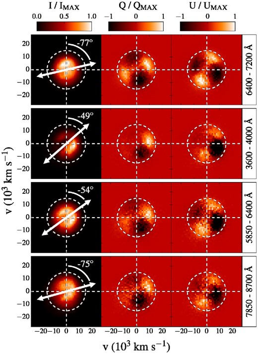
Colour maps of normalized I (left-hand panels), Q (middle panels) and U (right-hand panels) distributions projected on the plane perpendicular to the viewing angle |$\boldsymbol {n}_5$|⁠. The maps are computed selecting virtual packets escaping between 18.5 and 23.5 d after explosion and in the wavelength regions 6400–7200, 3600–4000, 5850–6400 and 7850–8700 Å (from top to bottom rows). White circles mark a projected velocity of 15 000 km s⁻¹. White arrows in the I maps indicate the electric field orientation obtained by calculating the polarization angle χ from the Q and U maps. The polarization angles derived for each spectral range are also reported.

Open in new tabDownload slide

Figure 7.

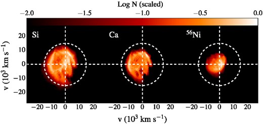
Colour maps of the silicon (left-hand panel), calcium (middle panel) and radioactive ⁵⁶Ni (right-hand panel) column densities N 100 s after explosion. These are calculated through the near-side hemisphere of the ejecta in the |$\boldsymbol {n}_5$| direction. The column density of each map has been scaled by the maximum value. White circles mark a projected velocity of 15 000 km s⁻¹.

Open in new tabDownload slide

4.2 Spectral evolution

In this section, we present the spectral time evolution for the violent merger model of Pakmor et al. (2012). To explore the range of polarization covered by the model, here we also include results of our simulation with 5 × 10⁷ Monte Carlo quanta and with polarization spectra extracted for an additional 30 viewing angles (see Section 3). In Section 4.2.1, we discuss the polarization evolution over the time interval between 10 and 30 d after explosion, while in Section 4.2.2 we investigate if changes in polarization for different orientations correlate with light-curve properties.

4.2.1 Polarization light curves

Figure 8.

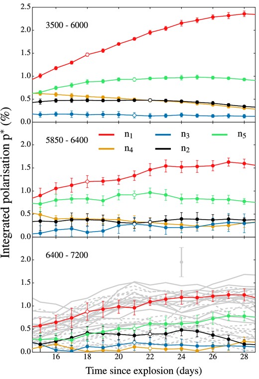
Polarization light curves between 15 and 28 d after explosion calculated in three different spectral range: 3500–6000 Å (top panel), 5850–6400 Å (middle panel) and 6400–7200 Å (bottom panel). Different colours refer to different viewing angles and the colour scheme for the observers |$\boldsymbol {n}_1{\rm -}\boldsymbol {n}_5$| is the same of Fig. 3. An additional 30 light curves (grey lines) are reported in the bottom panel and refer to a lower signal-to-noise (a factor of 4 fewer packets) calculation: solid lines are for observer orientations in a solid angle dΩ = 2π around the cavity in the IGE ejecta, while dashed lines stand for orientations on the opposite hemisphere. 1σ Monte Carlo noise error bars are derived following Bulla et al. (2015) and are larger for simulations carried out with fewer packets (grey lines). Open points mark the closest epoch to B-band maximum for the observers |$\boldsymbol {n}_1{\rm -}\boldsymbol {n}_5$|⁠.

Open in new tabDownload slide

4.2.2 Degree of polarization and light-curve properties

As illustrated by the polarization light curves (Fig. 8), the highest polarization signals correspond to observers out of the x–y plane for almost all epochs we considered. The fact that the system is also fainter from these observer orientations suggests that viewing-angle effects might cause a relationship between the degree of polarization and light-curve properties in the model. Wang, Baade & Patat (2007) have suggested that the peak polarization of the Si ii λ6355 line inversely correlates with luminosity for normal SNe Ia. Here we then examine if such a correlation could, in part, be driven by orientation effects in the model.

Wang et al. (2007) use a light-curve shape parameter, Δm₁₅(B), as a proxy for the SN luminosity. Specifically, the peak B-band absolute magnitude, M_{B, max}, and the magnitude decline in the B band from peak to 15 d after, Δm₁₅(B), have been shown to well correlate in normal SNe Ia, in the sense that brighter objects tend to decline more slowly (Phillips 1993; Phillips et al. 1999). Because of the strong asymmetries in the ejecta distribution, the explosion model of Pakmor et al. (2012) produces a wide range of M_{B, max} and Δm₁₅(B) values. Fig. 9 reports these two parameters for light curves extracted by binning the emergent Monte Carlo quanta in 100 solid angle bins. Only half of the points in this plot follow a trend close to the observed width–luminosity relation. In particular, about 70 per cent of the observers in a solid angle dΩ = 2π around the cavity deviate from the expected trend, suggesting that the influence of the secondary star might be negative on the model. In making comparisons of light-curve properties, in the following we will therefore (i) use M_{B, max} as the proxy for light-curve properties (since Δm₁₅(B) is known to be quite sensitive to the specific ionization treatment; see e.g. Kromer & Sim 2009 Dessart et al. 2014) and (ii) distinguish the points on the cavity side by using different symbols.

Figure 9.

Width–luminosity relation in our simulations. Individual points represent different orientations and are calculated by binning the escaping packets into 100 solid angle bins. Angular bins corresponding to the five orientations |$\boldsymbol {n}_1{\rm -}\boldsymbol {n}_5$| are shown with the same colour scheme used in Fig. 3, while grey points mark 30 orientations from a lower signal-to-noise calculation. Open symbols are points for which we did not carry out polarization synthesis. Points are also divided according to whether they are located in a solid angle dΩ = 2π around the IGE cavity (stars) or on the opposite side (circles). The observed trend from Phillips et al. (1999), M_{B, max} = M₀ + 0.786 [Δm₁₅(B) − 1.1] − 0.633 [Δm₁₅(B) − 1.1]², is shown with black lines. Different lines refer to different normalization factors M₀ at Δm₁₅(B) = 1.1: M₀ = −19.0 (solid line), M₀ = −19.2 (upper dashed line) and M₀ = −18.8 (lower dashed line).

Open in new tabDownload slide

To look for trends with M_{B, max}, in Fig. 10 we examine polarization levels integrated across the Si ii λ6355 line (between 5850 and 6400 Å) at 16 d after explosion, p*(16 d). This epoch is chosen as we aim to compare our predictions with the trend observed for normal SNe Ia 5 d before B-band maximum (Wang et al. 2007). To facilitate this comparison, we also convert the quantities presented by Wang et al. (2007) in the following way: (i) we translate Δm₁₅(B) into M_{B, max} values using the observed width–luminosity relation reported in Fig. 9 (M₀ = −19.0; Phillips et al. 1999); (ii) we transform the peak polarization of the Si ii λ6355 line into an integrated level between 5850 and 6400 Å assuming a Gaussian profile with full width at half-maximum of 150 Å.² As shown by Fig. 10, the correlation between luminosity and degree of polarization is moderate in our model (Pearson's coefficient r = 0.52) but is in the same sense as is suggested by the data: brighter viewing angles are typically less polarized and fainter viewing angles typically more polarized. The degrees of polarization predicted by our model, however, are typically stronger than those observed, and this discrepancy is found to be more pronounced for orientations on the side of the cavity.

Figure 10.

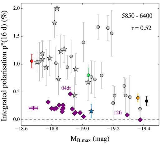
Integrated polarization across the Si ii λ6355 profile as a function of M_{B, max} (circles and stars). Polarization levels are extracted in the spectral range 5850–6400 Å at 16 d after explosion (about 5 d before B-band maximum). Individual points correspond to 35 different viewing angles and are marked and coloured as in Fig. 9. Error bars are estimated as in Bulla et al. (2015) and are larger for simulations that were carried out with a factor of 4 fewer packets (grey points). A Pearson coefficient r calculated including all the points is reported. After being properly converted (see the text), spectropolarimetric data of normal SNe Ia (Wang et al. 2007; Maund et al. 2013) are also plotted for comparison (purple diamonds). Purple error bars mark the averaged uncertainties for these values.

Open in new tabDownload slide

4.3 Comparison with SN 2004dt and SN 2012fr

Focusing on high signal-to-noise calculations, in this section we compare spectra extracted along |$\boldsymbol {n}_2-\boldsymbol {n}_5$| with spectropolarimetric data of SNe Ia. As shown in Sections 4.1 and 4.2, the degree of polarization for the model of Pakmor et al. (2012) is low (≲1 per cent) when the system is viewed equator-on (⁠|$\boldsymbol {n}_2$|⁠, |$\boldsymbol {n}_3$| and |$\boldsymbol {n}_4$|⁠) and higher for the viewing angle out of the equatorial plane (⁠|$\boldsymbol {n}_5$|⁠). Therefore, in the following, we present a comparison of our synthetic spectra with two normal SNe Ia showing different degrees of polarization: the highly polarized SN 2004dt (which we compare with predictions for the line of sight out of the equatorial plane) and the lowly polarized SN 2012fr (which we compare to our calculations in the equatorial plane).

4.3.1 SN 2004dt

Spectropolarimetric observations of SN 2004dt were triggered with the Focal Reducer and low dispersion Spectrograph (FORS1) at the ESO Very Large Telescope (VLT) 6–8 d before maximum (Wang et al. 2006) and with the Shane telescope at Lick Observatory 4 d after maximum (Leonard et al. 2005). The polarization signal detected across the Si ii λ6355 line was very prominent (2–2.5 per cent) and little evolution was observed between the two epochs.

In Fig. 11, we show observations of SN 2004dt together with synthetic spectra extracted at the corresponding epochs for the viewing angle |$\boldsymbol {n}_5$|⁠. Although the velocities in the model along |$\boldsymbol {n}_5$| are lower than those observed (e.g. ∼− 14 500 km s⁻¹ instead of ∼− 17 000 km s⁻¹ for the absorption trough of the Si ii λ6355 line 7 d before maximum), the simulated spectral shapes agree reasonably well with the data of SN 2004dt at both epochs. In particular, the agreement a week before maximum is remarkable. The polarization level in the pseudo-continuum range 6400–7200 Å is well reproduced and the predicted line polarization features are very similar to those observed. The match is particularly good for the silicon lines (e.g. Si ii λ3859,³ Si ii λ5979 and Si ii λ6355). In contrast, the model produces a degree of polarization that is too high in the region around 5000 Å.

Figure 11.

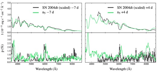
Flux and polarization spectra predicted for an observer orientation |$\boldsymbol {n}_5=({}^{1}/{\scriptsize 2},{}^{1}/{\scriptsize 2},{}^{1}/{\scriptsize\sqrt{2}})$|⁠. Spectra at −7 (left-hand panels) and +4 d (right-hand panels) relative to B-band maximum are shown with green lines. For comparison, black lines show observed spectra of SN 2004dt at the same epochs after correction for the interstellar polarization component (∼0.28 per cent; Leonard et al. 2005; Wang et al. 2006). Synthetic flux spectra are given for a distance of 1 Mpc, while flux spectra of SN 2004dt have been arbitrarily scaled for illustrative purposes.

Open in new tabDownload slide

Synthetic spectra 4 d after maximum are still consistent with data for SN 2004dt, though with stronger deviations. The most striking difference concerns the region across the Ca ii IR triplet feature, which appears to be too strong in the model. The fact that the calcium line is also prominent in the flux spectrum, however, suggests that the discrepancy might be ascribed to the simplified excitation/ionization approximation of artis (Kromer & Sim 2009), rather than only to the geometry of the model.

4.3.2 SN 2012fr

Spectropolarimetric data of SN 2012fr were acquired with FORS1 at ESO VLT at four different epochs: −11, −5, +2 and +24 d relative to B-band maximum (Maund et al. 2013). The degree of polarization of SN 2012fr was generally small, except for the signals associated with high- (early epochs) and low-velocity (late epochs) components of Si ii λ6355 and Ca ii IR lines. Maund et al. (2013) argued that the very low level of continuum polarization seen in SN 2012fr (<0.1 per cent) is not consistent with the asymmetric nickel distribution in the violent white dwarf mergers of Pakmor et al. (2012). Having undertaken a polarization spectral synthesis for this model, we can now investigate this comparison quantitatively.

In Fig. 12, we show spectropolarimetric data of SN 2012fr together with synthetic spectra extracted in the |$\boldsymbol {n}_4$| direction.⁴ The pseudo-continuum polarization at all epochs is fairly consistent⁵ with the level observed in SN 2012fr. This suggests that the strong asymmetries in the nickel distribution of Pakmor et al. (2012) might not necessarily lead to high polarization levels in the pseudo-continuum range (see also discussion in Section 4.1). However, the most striking discrepancy between the model and the data is the wealth of strong polarization features predicted in our simulation. As highlighted in Figs 3 and 4, these strong features are associated with the absorption troughs of spectral lines and are typically too strong to match the modest polarization signals of SN 2012fr. This fact suggests that the element distribution in the model ejecta is too asymmetric to account for the overall low levels of polarization observed in SN 2012fr and similar SNe Ia.

Figure 12.

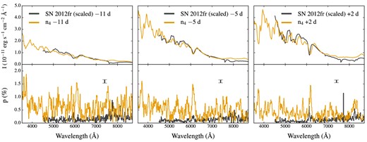
Flux and polarization spectra predicted for an observer orientation |$\boldsymbol {n}_4=({}^{1}/{\scriptsize\sqrt{2}},{}^{1}/{\scriptsize\sqrt{2}},0)$|⁠. Spectra at −11 (left-hand panels), −5 (middle panels) and +2 d (right-hand panels) relative to B-band maximum are shown with orange lines. For comparison, black lines show observed spectra of SN 2012fr at the same epochs after correction for the interstellar polarization component (∼0.24 per cent; Maund et al. 2013). Black bars mark the averaged errors in the observed spectra at each epoch. Synthetic flux spectra are given for a distance of 1 Mpc, while flux spectra of SN 2012fr have been arbitrarily scaled for illustrative purposes.

Open in new tabDownload slide

In Fig. 13, we compare observations of SN 2012fr with the spectra predicted by our model in the |$\boldsymbol {n}_3$| direction. As previously noticed, the degree of polarization associated with this orientation is typically weaker compared to the other two equatorial orientations that we have considered, and thus it provides better agreement, although still imperfect, if one considers only polarization. However, the flux spectra extracted for this direction are characterized by very broad and shallow features that are not consistent with the observations of SN 2012fr.

Figure 13.

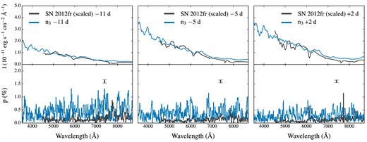
Same as Fig. 12 for an observer orientation |$\boldsymbol {n}_3=(-{}^{1}/{\scriptsize\sqrt{2}},-{}^{1}/{\scriptsize\sqrt{2}},0)$|⁠.

Open in new tabDownload slide

5 DISCUSSION AND CONCLUSIONS

We have presented a polarization spectral synthesis analysis of the violent merger of a 1.1 and a 0.9 M_⊙ carbon–oxygen white dwarf (Pakmor et al. 2012). Using a technique recently implemented in the Monte Carlo radiative transfer code artis (Bulla et al. 2015), we have calculated polarization spectra for multiple observer orientations between 10 and 30 d after explosion. Our simulations focused on five orientations, for which a large number of Monte Carlo quanta were used in order to extract detailed synthetic observables. Results for those five orientations are supplemented by 30 additional, lower signal-to-noise calculations that allowed us to map out the range of polarization covered by the model.

Around maximum light, the overall degree of polarization for viewing angles in the equatorial plane is relatively low (p ≲ 1 per cent). Polarization spectra clearly identify the dominant axis of the model, reflecting the overall symmetry of the ejecta about the x–y plane. In contrast, higher polarization levels and departures from a single-axis geometry are found for viewing angles out of the equatorial plane. For a given observer, polarization angles estimated across Si ii lines differ from those across Ca ii lines, reflecting the distinct morphologies of silicon and calcium in the ejecta.

Focusing on high signal-to-noise calculations, we compared our synthetic spectra with spectropolarimetric data of two normal SNe Ia: the highly polarized SN 2004dt (Leonard et al. 2005; Wang et al. 2006) and the lowly polarized SN 2012fr (Maund et al. 2013). Synthetic spectra extracted along the direction |$\boldsymbol {n}_5=({}^{1}\!/_{2},{}^{1}\!/_{2},{}^{1}\!/\!_{\sqrt{2}})$| provide a good match to those of SN 2004dt at −7 and + 4 d relative to B-band maximum. In particular, the match is remarkable one week before maximum, with the signals across the Si ii and Ca ii profiles and in the continuum range found to be very similar to those observed. In contrast, none of the equatorial viewing angles can simultaneously reproduce the polarization and intensity spectra observed in SN 2012fr. Owing to the strong asymmetries in the element distribution, the model predicts a wealth of strong (∼1 per cent) polarization lines both in the blue and in the red part of the spectrum, in contrast with the behaviour commonly observed in SNe Ia.

In addition, we found that about half of the 35 orientations investigated in this study clearly deviate from the trend observed in SNe Ia, with polarization levels that are typically too high and still increasing ∼10 d after maximum light. Interestingly, most of these orientations are oriented close to the cavity in the ⁵⁶Ni distribution, which is filled by material from the companion star. The negative impact of the material from the explosion of the companion star on the model is also suggested by the identification in our spectra of two optical C ii lines at rather low velocities (v ∼ −6800 km s⁻¹). These features, associated with unburned carbon material from the companion, are not normally observed at such low velocities (v_obs ∼ −12 000 km s⁻¹; Parrent et al. 2011; Thomas et al. 2011) or detected in polarization (see e.g. Wang & Wheeler 2008).

With this paper, we have started our project aimed to predict polarization signatures for a set of contemporary SN Ia explosion models. We have investigated the particular model of Pakmor et al. (2012) and shown that this violent merger of a 1.1 and 0.9 M_⊙ carbon–oxygen white dwarf might account for some highly polarized objects such as SN 2004dt but not for the typical behaviour observed in SNe Ia. In particular, our study consistently finds that the discrepancies can be attributed to the location and nature of the ashes of the companion star. Future studies will focus on studying polarization signatures for other existing merger models (e.g. Kromer et al. 2013; Pakmor et al. 2013) and on investigating alternative scenarios with revised explosion/secondary properties (e.g. different mass ratios, a different location and time of ignition or a larger distance between the two stars). This might reduce the ejecta asymmetries and thus lead to better agreement with spectropolarimetric data of SNe Ia.

The authors are thankful to Douglas Leonard and Justyn Maund, for providing the spectropolarimetric data of SN 2004dt and SN 2012fr reported in this paper, and to Nando Patat, Lifan Wang and Craig Wheeler for useful discussions.

SAS acknowledges support from STFC grant ST/L000709/1, RP by the European Research Council under ERC-StG grant EXAGAL-308037, and WH and ST by TRR 33 ‘The Dark Universe’ of the German Research Foundation (DFG). FKR acknowledges support by the DAAD/Go8 German-Australian exchange programme, and by the ARCHES prize of the German Ministry of Education and Research (BMBF). IRS was supported by the Australian Research Council Laureate Grant FL0992131.

This work used the DiRAC Complexity system, operated by the University of Leicester IT Services, which forms part of the STFC DiRAC HPC Facility (www.dirac.ac.uk). This equipment is funded by BIS National E-Infrastructure capital grant ST/K000373/1 and STFC DiRAC Operations grant ST/K0003259/1. DiRAC is part of the National E-Infrastructure.

This research was supported by the Partner Time Allocation (Australian National University), the National Computational Merit Allocation and the Flagship Allocation Schemes of the NCI National Facility at the Australian National University. Parts of this research were conducted by the Australian Research Council Centre of Excellence for All-sky Astrophysics (CAASTRO), through project number CE110001020.

REFERENCES