


Abstract
The estimation of cosmological constraints from observations of the large-scale structure of the Universe, such as the power spectrum or the correlation function, requires the knowledge of the inverse of the associated covariance matrix, namely the precision matrix, |$\boldsymbol {\Psi }$|. In most analyses, |$\boldsymbol {\Psi }$| is estimated from a limited set of mock catalogues. Depending on how many mocks are used, this estimation has an associated error which must be propagated into the final cosmological constraints. For future surveys such as Euclid and Dark Energy Spectroscopic Instrument, the control of this additional uncertainty requires a prohibitively large number of mock catalogues. In this work, we test a novel technique for the estimation of the precision matrix, the covariance tapering method, in the context of baryon acoustic oscillation measurements. Even though this technique was originally devised as a way to speed up maximum likelihood estimations, our results show that it also reduces the impact of noisy precision matrix estimates on the derived confidence intervals, without introducing biases on the target parameters. The application of this technique can help future surveys to reach their true constraining power using a significantly smaller number of mock catalogues.
INTRODUCTION
The small statistical uncertainties associated with current cosmological observations allow for precise cosmological constraints to be derived (e.g. Anderson et al. 2014; Planck Collaboration 2015). Future stage IV experiments such as Euclid (Laureijs et al. 2011) and the Dark Energy Spectroscopic Instrument (DESI; Eisenstein & DESI Collaboration 2015) will push the attainable level of precision even further, providing a strong test of the standard Λ cold dark matter (ΛCDM) cosmological model.
As statistical uncertainties are reduced, the control of potential systematic errors becomes essential to derive robust cosmological constraints. Besides the correct treatment of the observations and accurate models of the data, precision cosmology requires a thorough control of the assumptions made when establishing the link between theory and observations. For example, most analyses of clustering statistics assume a Gaussian likelihood function. This assumption must be carefully revised as they might introduce systematic biases on the obtained confidence levels (Kalus, Percival & Samushia 2015).
Even for the Gaussian case, the evaluation of the likelihood function requires the knowledge of the precision matrix, Ψ, that is, the inverse of the covariance matrix of the measurements. In most analyses of clustering measurements, the precision matrix is estimated from an ensemble of mock catalogues reproducing the selection function of each survey (e.g. Manera et al. 2013, 2014). However, all estimates of Ψ based on a finite number of mock catalogues are affected by noise. A rigorous statistical analysis requires the propagation of these uncertainties into the final cosmological parameter constraints.
Recent studies have provided a clear description of the dependence of the noise in the estimated precision matrix on the number of mock catalogues used (Taylor, Joachimi & Kitching 2013), its propagation to the derived parameter uncertainties (Dodelson & Schneider 2013; Taylor & Joachimi 2014) and the correct way to include this additional uncertainty in the obtained cosmological constraints (Percival et al. 2014). The results from these studies show that, depending on the number of bins of a given measurement, a large number of mock catalogues might be necessary in order to keep this additional source of uncertainty under control. For future large-volume surveys such as Euclid or DESI, this requirement might be infeasible, even if these are based on approximated methods such as pinocchio (Monaco, Theuns & Taffoni 2002), cola (Tassev, Zaldarriaga & Eisenstein 2013; Koda et al. 2015), patchy (Kitaura, Yepes & Prada 2014) or ezmocks (Chuang et al. 2015) instead of full N-body simulations.
In this paper, we test the implementation of the covariance tapering (CT) method (Kaufman, Schervish & Nychka 2008) as a tool to minimize the impact of the noise in precision matrix estimates derived from a finite set of mock catalogues. Although this technique was originally designed as a way to speed up the calculation of maximum likelihood estimates (MLE), we show that this method can also be used to reduce the noise in the estimates of the precision matrix. The CT approach can help to obtain parameter constraints that are close to ideal (i.e. those derived when the true covariance matrix is known) even when the precision matrix is estimated from a manageable number of realizations. Our results show that CT can significantly reduce the number of mock catalogues required for the analysis of future surveys, allowing these data to reach their full constraining power.
The structure of the paper is as follows. In Section 2, we summarize the results of previous works regarding the impact of the noise in precision matrix estimates on cosmological constraints. The CT technique is described in Section 3. In Section 4, we apply CT to the same test case studied by Percival et al. (2014), that of normally distributed independent measurements of zero mean. We then extend this analysis to a case with non-zero intrinsic covariances. Section 5 presents a study of the applicability of CT to the measurement of the baryon acoustic oscillations (BAO) signal using Monte Carlo realizations of the large-scale two-point correlation function. Finally, in Section 6 we present our main conclusions.
IMPACT OF PRECISION MATRIX ERRORS ON COSMOLOGICAL CONSTRAINTS
As this approach is based on a finite number of realizations, the estimator in equation (4) will be affected by noise (Taylor et al. 2013), whose effect must be propagated into the obtained constraints on the target parameters. The accuracy of the obtained confidence levels on the parameters |${\boldsymbol \theta }$| and their respective covariances is then ultimately limited by the uncertainties in the estimated precision matrix |$\boldsymbol {\hat{\Psi }}$| (Taylor & Joachimi 2014).
Taylor & Joachimi (2014) derived general formulae for the full propagation of the noise due to the finite sampling of the data covariance matrix into the parameter covariance estimated from the likelihood width and peak scatter estimators, which do not coincide unless the data covariance is exactly known. Their results are in good agreement with the second-order approximations of Dodelson & Schneider (2013) and Percival et al. (2014) in the regime of Ns ≫ Nb ≫ Np, but show deviations from these results for smaller number of simulations.
In the large Ns limit, the correction factor of equation (7) can be used to obtain constraints that correctly account for the additional uncertainty due to the noise in the precision matrix estimate of equation (4). However, this additional uncertainty in the parameter covariance matrix, hinders the constraining power of the data. Given the number of bins in a measurement |${\boldsymbol D}$| and the number of parameters that one wishes to explore, the correction factor of equation (5) can be used to estimate the number of synthetic measurements required to reach a given target accuracy in the derived constraints. If the number of bins in a given measurement is large, as could be the case for anisotropic or tomographic clustering measurements, the required number of mock realizations to keep the additional uncertainty under control might become infeasible. The aim of our analysis is to test a new technique to reduce the impact of the uncertainties in |${\hat{\boldsymbol \Psi }}$| on the final parameter constraints, which could help to significantly relieve these requirements.
COVARIANCE TAPERING FOR LIKELIHOOD-BASED ESTIMATION
In this section, we describe the CT technique developed by Kaufman et al. (2008) to improve the efficiency on the computation of MLE. This method was first applied to clustering measurements in Paz et al. (2013). The original idea behind CT is the fact that, in many applications, the correlation between data pairs far apart is negligible and little information is lost by treating these points as being independent. In this case, setting their corresponding elements in the covariance matrix to be exactly zero makes it possible to take advantage of fast numerical methods for dealing with sparse matrices, leading to a significant speed-up of the evaluation of the likelihood function.
However, in this work we focus on a different use of CT. The off-diagonal elements of the covariance matrix of a general measurement might exhibit a wide range of values and uncertainties. Even when these elements are non-negligible, their relevance to obtain an accurate description of the likelihood function must be assessed in terms of their associated errors. In this way, by down-weighting the contribution of these points (which typically have a low signal-to-noise ratio) to the estimated precision matrix it is possible to avoid the propagation of errors into the final cosmological constraints.
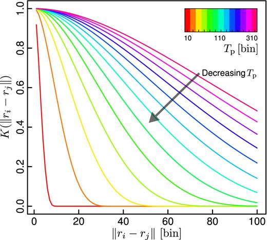
The behaviour of the family of tapering functions used in this work (the Wendland 2.0 function class) corresponding to different values of the tapering parameter Tp. The abscissas represent the distance between two measurement locations (denoted by ri) in data set space, which are shown in units of data ordinals (i.e bin units, ri ≡ i). Larger values of Tp result in functions with a larger support interval.
The likelihood is then estimated by replacing |$\boldsymbol {\Psi }$| in equation (1), by the two-tapered precision matrix estimator,|$\boldsymbol {\Psi ^\mathrm{t}}$|. In the following sections, we will show that the CT method is not only useful to approximate the MLE in a more computationally efficient way, as shown in Kaufman et al. (2008). As we will see, CT is also an appropriate technique to significantly reduce the impact of the noise in the precision matrix estimated from a set of mock measurements, increasing in this way the precision of the obtained likelihood confidence regions.
COVARIANCE TAPERING IN PRACTICE
Testing CT on independent normal-distributed measurements
In this section, we compare the performance of the CT approach with the standard MLE method when applied to the case of Nb independent normal-distributed random variables, in a similar analysis to those performed by Dodelson & Schneider (2013), Taylor et al. (2013) and Percival et al. (2014). This simple test is able to illustrate how the CT technique can be used to minimize the effects of covariance errors on the estimation of likelihood confidence intervals.
Our data set for this test consists of Nb Gaussian numbers with null mean and standard deviation equal to unity, in which case the covariance matrix is given by the Nb × Nb identity matrix. However, we perform a MLE of the sample mean, μ, without assuming any data independence. We first compute |$\hat{\sf{C}}$| from a set of Ns independent Monte Carlo realizations of Nb independent Gaussian numbers |$D^s_i$|. This estimate can be used to obtain |$\boldsymbol {\hat{\Psi }}$| and |$\boldsymbol {\Psi ^t}$| using equations (3) and (12). Both of these estimates will include ‘apparent’ correlations between different bins, due to the noise in the off-diagonal elements. We generate an additional independent set of Nb Gaussian numbers to be used as the data set for the target parameter estimation. The estimation of the sample mean is achieved by maximizing the likelihood function in equation (1). In this case the model is quite simple, a constant function Ti(μ) = μ. This procedure is repeated 105 times, obtaining an estimation for the target parameter on each time. By using the set of all the estimated values of μ we are able to compute the standard error σ achieved by the MLE method. The use of an independent data set on parameter estimation, employing the first Ns samples for the estimation of |$\hat{\sf{C}}$|, gives an unbiased set of target parameter estimations (Percival et al. 2014).
The results of this test are shown in Fig. 2, where the open points correspond to the parameter variance obtained when the standard technique is used, i.e. the precision matrix is approximated by |$\boldsymbol {\hat{\Psi }}$|, for the case of Nb = 15. The comparison of these results with the dotted line, which corresponds to the true expected variance of the mean of a Gaussian random variable, illustrates the effect of the noise in the covariance matrix. As can be seen, the variance decreases as Ns increases, which is expected due to the corresponding improvement on the |$\hat{\sf{C}}$| estimations. This behaviour is well described by the formulae given in Dodelson & Schneider (2013), as can be seen by looking at the dashed line in Fig. 2. The same behaviour has been seen over a wide range of Nb. The agreement found here is consistent with the results of Taylor & Joachimi (2014), given that the cases considered here correspond to the regime of large Ns compared to the number of parameters and data bins used. The solid line corresponds to the variance obtained when the precision matrix is estimated using |$\boldsymbol {\Psi ^\mathrm{t}}$| of equation (12) with a tapering scale of 10 bins. The application of the CT method significantly reduces the impact of the noise in the variance of the target parameter, leading to results that are much closer to those of the ideal case.
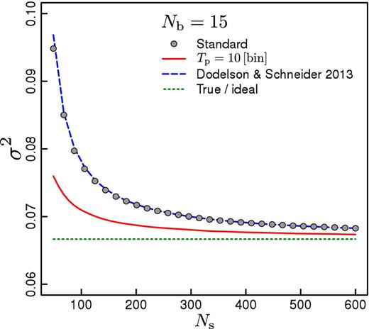
Variance of 105 MLE of the mean of sets of Nb = 15 uncorrelated normal random variables, as a function of the number of independent data realizations used on estimation of the precision matrix. Open symbols correspond to the variance obtained when the standard method is used (i.e. the precision matrix is approximated by |$\boldsymbol {\hat{\Psi }}$|). The dashed line shows the results obtained when applying the CT technique (i.e. the precision matrix is approximated by |$\boldsymbol {\Psi ^\mathrm{t}}$|) with a tapering parameter of 10 bins. The solid line corresponds to the analytic formulae given in Dodelson & Schneider (2013). The dotted line correspond to the expected variance for the mean of uncorrelated Gaussian random variables with first and second moment equal to zero and one, respectively.
Testing the CT method for realistic covariances
In the previous section, we tested the results obtained by applying CT in an ideal case in which the true covariance matrix is diagonal. In this section, we extend this test by considering the case in which the different elements of the data set have non-negligible correlations. To this end, we generate Monte Carlo realizations of Nb Gaussian random variables with zero mean, correlated following a realistic model of the covariance matrix of the two-point correlation function (Sánchez, Baugh & Angulo 2008). The upper triangular of the top-left panel of Fig. 3 shows the model for the covariance matrix for the case of Nb = 50, normalized as indicated in the figure key (that is, the correlation matrix). For comparison, the lower triangular part of the same panel shows the estimate |$\hat{\sf{C}}$| obtained using 300 independent Monte Carlo realizations. As can be seen, the main features of the model covariance matrix are recovered. However, the presence of noise is clear in the off-diagonal elements of the matrix, corresponding to covariances of measurements at large separations. The signal-to-noise ratio of the covariance matrix is smaller for the off-diagonal elements. The main idea of this work is to control the propagation of these errors into the precision matrix, restricting in this way their impact on the likelihood function and the obtained confidence intervals of the target parameters.
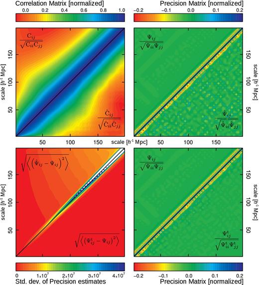
Top-left panel: comparison between the model for the covariance matrix used in this work (upper triangular part) and the standard estimation using 300 realizations. Top-right panel: the true precision matrix |$\boldsymbol {\Psi }$| (the matrix inverse of the model, upper triangular part) compared to the usual estimator |$\boldsymbol {\hat{\Psi }}$|. Bottom right panel: as in the above panel, but comparing this time |$\boldsymbol {\Psi }$| with the CT estimator |$\boldsymbol {\Psi ^\mathrm{t}}$| using Tp = 230 h−1 Mpc. Bottom left panel: standard deviations for 104 precision matrix estimates, with (lower triangular part) and without CT (upper triangular part), around the true matrix |$\boldsymbol {\Psi }$|.
The top-right panel of Fig. 3 shows the precision matrices corresponding to the model for the covariance matrix (upper triangular part) and the one obtained using the standard estimator of equation (4), normalized in analogous manner to the covariance matrices. As can be seen, the presence of noise in the off-diagonal elements is even more remarkable in the case of the precision matrix. The increment on the noise is due to the propagation of errors during the matrix inversion operation. The bottom-right panel of Fig. 3 shows a comparison of the precision matrix obtained by applying CT with a tapering parameter Tp = 230 h−1 Mpc (lower triangular part) and the model precision matrix (upper triangular part, identical to the one shown in the upper part of the top-right panel). The application of CT leads to a significant suppression of the noise in the off-diagonal elements of the precision matrix.
The improvement in the accuracy obtained by applying CT can be quantified by computing the deviations of the different estimators from the true model precision matrix. The lower-left panel of Fig. 3, shows the standard deviations, element by element, of the estimators |$\boldsymbol {\hat{\Psi }}$| and |$\boldsymbol {\Psi ^t}$| for Ns = 300, with respect to the ideal precision matrix. The upper triangular part corresponds to the deviations obtained using the standard method (which are well approximated by the analytic formulae given in Taylor et al. 2013), whereas the lower triangular part shows the results obtained using the CT technique. The standard deviations obtained when CT is applied are smaller than those achieved by the standard technique, indicating a better performance at recovering the correct underlying precision matrix.
The success of the CT method depends on the selection of an adequate tapering scale Tp. In the case analysed in this section, a natural way to characterize the different approaches is through the recovered error in the mean μ. The ideal error, which represent the true constraining power of a given data set, can be easily computed by taking the inverse of the single element of the fisher matrix. As the derivative of the model with respect to the target parameter is 1 for each of the Nb dimensions, the ideal error of the mean is simply given by σideal = 1/∑ijΨij. Fig. 4 shows a comparison between the standard and CT methods for a fixed number of bins and simulations (Nb = 30, Ns = 100). For each method, we show the ratio σμ/σideal. The solid line corresponds to the results obtained by applying CT as a function of the tapering scale Tp. The dashed line shows to the error obtained using the standard method, where the precision matrix is estimated by |$\boldsymbol {\hat{\Psi }}$|. The standard deviation obtained in this case corresponds to an excess of 45 per cent with respect to that of the ideal case, indicated by the dotted line. As can be seen, there is an optimal tapering scale of Tp ≃ 230 h−1 Mpc), for which the error obtained is only 10 per cent larger than the ideal value. For large tapering scales, the CT method recovers the same results as the standard technique, whereas for small Tp the errors become larger again. This behaviour might be given by the relation between the tapering scale and the structure of the off-diagonal elements of the covariance matrix. For large values of Tp, the tapering procedure damps the contribution of the most off-diagonal elements of the covariance matrix, whose intrinsic values are small and are dominated by noise. As the tapering scale is reduced, the damping of the noise is more efficient and the results become more similar to those of the ideal case. However, if the tapering scale is too small, this procedure might affect entries of the covariance matrix whose intrinsic values are not small. As these off-diagonal elements are affected, the obtained results deviate again from those of the ideal case.
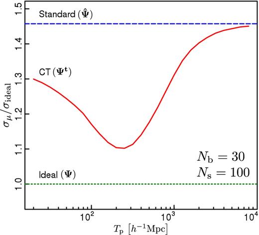
Error of the mean of Nb = 30 random Gaussian numbers with zero mean and covariance given by the model of Sánchez et al. (2008), normalized to the ideal error σideal predicted by the model. The dashed line corresponds to the error obtained using the standard method, where the |$\boldsymbol {\hat{\Psi }}$| estimator is taken as a proxy of the ideal precision matrix. The solid line shows the results corresponding to the CT technique, where the precision matrix is estimated by |$\boldsymbol {\Psi ^\mathrm{t}}$|. The dotted line corresponds to the ideal error.
In Fig. 5, we show the results of extending this test to a wide range of Ns values. The variance of the MLE of the mean of 105 independent data sets of Nb = 30 correlated Gaussian numbers is shown as a function of the number of realizations employed in the estimation of |$\hat{\sf{C}}$|. The points correspond to the variance inferred using the standard technique, whereas the solid coloured lines indicate the results obtained by applying CT with different Tp values, as indicated in the figure key. The dashed line corresponds to the expected ideal variance of the mean, |$\sigma ^2_\mathrm{ideal}$|. As can be seen in the left-hand panel of this figure, the variance recovered by applying CT with large tapering scales is very similar to the result of the standard method. However, as the tapering scale decreases, the variance also becomes smaller, reaching values close to those of the ideal case for Tp ≃ 230 h−1 Mpc. The lower panels in Fig. 5 show the behaviour of the estimated values of the target parameter for the standard (points) and CT (solid lines) methods. In all cases the recovered values of μ show no indication of a systematic deviation from the true value μ = 0, with only small fluctuations for different values of Ns.

Variance of 105 MLE of the mean of Nb Gaussian numbers, following a realistic model of the covariance. The results are presented as a function of the number of samples used in the covariance estimation. Open symbols correspond to the variance obtained when the precision matrix is estimated through the standard method (i.e. |$\boldsymbol {\hat{\Psi }}\rightarrow \boldsymbol {\Psi }$|). Solid coloured lines show the results obtained by CT using different Tp parameter values, as indicated in the key. The dashed line correspond to the expected variance for the mean, that is the inverse of the fisher element. Left-hand panel corresponds to Tp values between 230 and 3330 h−1 Mpc, whereas right-hand panel shows the results of Tp ranging from 66 to 230 h−1 Mpc. The bottom subpanels at both sides show the recovered μ values for all methods.
The right-hand panel of Fig. 5 shows the results obtained by applying the CT technique for values of the tapering scale of less than 230 h−1 Mpc, which result in larger variances of the target parameter. However, it is worth noticing that even in this case there is no bias in the obtained constraints. These results suggest that the optimal tapering scale depends only on the shape of the underlying covariance matrix, rather than the number of independent data samples used to compute |$\boldsymbol {\hat{C}}$|.
APPLICATION TO BARYON ACOUSTIC OSCILLATION MEASUREMENT
In this section, we analyse the applicability of the CT method, in the context of BAO measurements. For this test, we use the model of the full shape of the large-scale two-point correlation function, ξ(s), of Sánchez et al. (2013, 2014), which is based on renormalized perturbation theory (Crocce & Scoccimarro 2006). We generate sets of correlated Gaussian numbers with mean given by the model of ξ(s) and the same covariance matrix as in the test of the previous section (Sánchez et al. 2008). In this way, each Monte Carlo realization mimics a realistic measurement of the correlation function at the scales relevant for BAO measurements.
The procedure described above is repeated 2 × 10⁵ times to obtain a smooth measurement of the dispersion of the α values obtained from different realizations. Fig. 6 shows the behaviour of this dispersion as a function of the number of mock samples used in the estimation of the covariance matrix. The points correspond to the results obtained when the precision matrix is approximated by the estimator |$\boldsymbol {\hat{\Psi }}$| of equation (3). As expected, the error in α decreases as Ns increases, approaching the ideal error obtained when the true covariance matrix is used to evaluate the likelihood function, shown by the black solid line. The results from our Monte Carlo realizations are well described by the analytic formulae given by Dodelson & Schneider (2013), which is shown by the blue short-dashed line. The red long-dashed line corresponds to the result of rescaling the mean variance on α recovered from each MCMC by the correction factor of equation (7) which, as shown by Percival et al. (2014), correctly accounts for the additional error due to the noise in |$\boldsymbol {\hat{C}}$|.
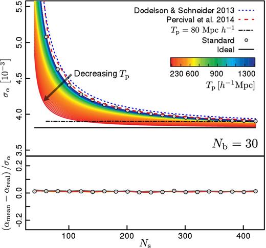
Standard deviation of the BAO peak scale as a function of the number of simulations used in the covariance estimate (upper panel). Open circles indicate the results corresponding to the standard method. Long and short dashed lines corresponds to the analytic formulae of Dodelson & Schneider (2013) and Percival et al. (2014). The black solid line indicates the error obtained when the ideal precision matrix is used. Coloured lines (from blue to red) show the results obtain by applying CT with different tapering scales. The black dot–dashed line show the CT results when a too small tapering parameter is used (Tp = 80 h−1 Mpc).
The thin solid lines in Fig. 6 correspond to the results obtained using the CT method, colour-coded according to the corresponding tapering scale. For large tapering scales the results closely resemble those of the standard technique. As the tapering parameter decreases, approaching the optimal scale found in the previous section of 230 h−1 Mpc, the dispersion of the BAO scale estimates becomes closer to the ideal error. These results show that, for a given value of Ns, the CT method leads to measurements of the BAO scale that are closer to the true constraining power of the data than the standard technique. For Ns ≃ 400 the uncertainty obtained using the CT method essentially recovers that of the ideal case.
The black dot–dashed line in Fig. 6 corresponds to the CT results obtained by setting Tp = 80 h−1 Mpc, illustrating the effect of implementing a too small tapering scale. As we found in the previous section, selecting a too small tapering scale leads to an increment of the errors in the target parameters. However, as shown in the lower panel of Fig. 6, even in this case the CT results show no systematic bias, with negligible differences from the true underlying parameter αtrue = 1 for the full range of Ns values analysed.
The improvement of the constraints achieved by the CT technique with respect to the standard method ultimately relays in a closer approximation of the ideal likelihood surface. In Fig. 7, we show the difference between the mean marginalized posterior distribution of the shift parameter α obtained by applying CT with different tapering scales (green and purple lines, as indicated in the figure key) and that of the ideal case. The posterior distribution corresponding to the standard method is shown as a solid orange curve. In general, the CT results provide a closer approximation of the ideal distribution than the standard method, most notably for a tapering scale of 230 h−1 Mpc. The use of a larger tapering scale leads to larger deviations from the ideal likelihood function. However, in all of these cases they are closer to the optimal result than the standard method. In contrast, using a too small tapering scales (as in the case of Tp = 50 h−1 Mpc shown in the figure) leads to deviations from the underlying likelihood function that can be even larger than those obtained with the standard technique. This highlights the importance of performing a careful analysis of the optimal tapering scale for each case, which will depend on the structure of the covariance matrix.
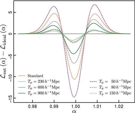
Difference between the mean marginalized posterior distribution of the shift parameter α obtained by applying CT with different tapering scales (green and purple lines) and that of the ideal case (grey line). The orange curve shows the results obtained by the standard method.
SUMMARY AND CONCLUSIONS
In this work, we have implemented and tested a novel technique for the estimation of the precision matrix, the CT method, developed by Kaufman et al. (2008). We have analysed the performance of the CT method and the standard technique by comparing the obtained parameter constraints with those found in the ideal case where the true precision matrix is known. For the latter case, the size of the errors in the estimated parameters is only governed by the constraining power of the data sample. Therefore, any excess seen in the recovered errors in comparison with that of the ideal case can be associated with the noise in the precision matrix estimation.
We first carried out an analysis similar to those performed by Dodelson & Schneider (2013), Taylor et al. (2013) and Percival et al. (2014), using the standard deviation of the maximum likelihood estimation of the mean of Nb independent normal random variables as a test case. Our results are in agreement with previous works, indicating that the noise in the covariance matrix estimation has a significant impact on the uncertainty obtained on parameter constraints. We found that the size of the synthetic data set used to estimate the precision matrix is crucial to control the impact of the covariance uncertainties on the final parameter constraints. Our results also show that CT helps to reduce the error in the precision matrix estimation, leading to uncertainties in the target parameters that are closer to the ideal case than those obtained with the standard method.
The efficiency of the CT technique for a data set composed of independent normal variables, where the true covariance matrix is diagonal, can be expected. In order to check the validity of the CT method in a more realistic situation, we also studied the case of the MLE of the mean of Gaussian numbers with non-zero correlations given by a realistic model of the covariance matrix of the two-point correlation function (Sánchez et al. 2008). Our results show that also in this case the CT method leads to smaller errors than the standard technique, without introducing any systematic bias in the estimated parameters. In this case we found an optimal tapering scale, defined as the value of the tapering parameter for which the obtained standard deviation is closer to its ideal value. For example, in the case of 30 normal distributed values and 100 synthetic samples on the covariance estimation, the CT method with the optimal tapering scale, gives a standard deviation only 10 per cent larger than that of the ideal case, whereas the standard technique results in errors 45 per cent larger. We showed that the optimal tapering parameter depends only on the structure of the underlying covariance matrix and is insensitive to the bin size or the number of synthetic samples used in the estimation of the precision matrix. Smaller tapering parameters than the optimal value result in an increase of the standard deviation, although no bias is introduced.
Finally, we performed an analysis of the CT technique on a more realistic context by testing its applicability to isotropic BAO measurements. We used an accurate model of the large-scale two-point correlation function (Sánchez et al. 2013) and its full covariance matrix (Sánchez et al. 2008) to generate Monte Carlo realizations of this quantity. We used these synthetic measurements to perform fits of the BAO signal following the methodology of Anderson et al. (2014). We found that the CT method significantly reduces the impact of the noise in the precision matrix on the obtained errors in the BAO peak position without introducing any systematic bias. As in the previous case, the optimal tapering parameter only depends on the shape of the true covariance matrix, with a preferred Tp scale similar to that of the previous test (i.e. the case of zero-mean correlated Gaussian numbers).
CT can help to reduce the required number of mock catalogues for the analysis of current and future galaxy surveys. This can be clearly illustrated by extending the analysis of Section 5 to the case of Ns = 600, corresponding to the number of mock catalogues used in the analysis of the SDSS-DR9 BOSS clustering measurements of Anderson et al. (2012). In this case, the uncertainty in the BAO shift parameter obtained by applying the CT technique is equivalent to that derived with the standard method using Ns = 2300 instead.
As we highlighted before, the performance of the CT technique ultimately depends on the structure of the underlying covariance matrix. In this work, we assumed a Gaussian model for the covariance matrix of the correlation function. Although this model gives an excellent description of the results of numerical simulations, more accurate models must include also the contribution from modes larger than the survey size (de Putter et al. 2012) or non-Gaussian terms (Scoccimarro, Zaldarriaga & Hui 1999) that would affect the off-diagonal elements of the covariance matrix. We leave the study of the performance of the CT under the presence of these contributions for future work, as well as the extension of the present analysis to alternative data sets such as the power spectrum or anisotropic clustering measurements in general.
The CT technique can be extremely useful for the analysis of future surveys such as Euclid and DESI. The small statistical uncertainties associated with these data sets will provide strong tests for the standard ΛCDM cosmological model. However, the large number of mock catalogues that are required by the standard technique to maintain the accuracy level of the cosmological constraints might be infeasible. The application of the CT technique can significantly reduce the number of mock catalogues required for the analysis these surveys, allowing them to reach their full constraining power.
The authors are thankful to Andrés Nicolás Ruiz and Salvador Salazar-Albornoz for useful discussions and suggestions about this manuscript. DJP acknowledges the support from Consejo Nacional de Investigaciones Científicas y Técnicas de la República Argentina (CONICET, project PIP 11220100100350) and the Secretaría de Ciencia y Técnica de la Universidad Nacional de Córdoba (SeCyT, project number 30820110100364). DJP also acknowledges the hospitality of the Max-Planck-Institut für extraterrestrische Physik were part of this work was carried out. AGS acknowledges the support from the Trans-regional Collaborative Research Centre TR33 ‘The Dark Universe’ of the German Research Foundation (DFG).
REFERENCES
