


Abstract
Cyclotron resonance scattering features observed in the spectra of some X-ray pulsars show significant changes of the line centroid energy with the pulsar luminosity. Whereas for bright sources above the so-called critical luminosity, these variations are established to be connected with the appearance of the high-accretion column above the neutron star surface, at low, sub-critical luminosities the nature of the variations (but with the opposite sign) has not been discussed widely. We argue here that the cyclotron line is formed when the radiation from a hotspot propagates through the plasma falling with a mildly relativistic velocity on to the neutron star surface. The position of the cyclotron resonance is determined by the Doppler effect. The change of the cyclotron line position in the spectrum with luminosity is caused by variations of the velocity profile in the line-forming region affected by the radiation pressure force. The presented model has several characteristic features: (i) the line centroid energy is positively correlated with the luminosity; (ii) the line width is positively correlated with the luminosity as well; (iii) the position and the width of the cyclotron absorption line are variable over the pulse phase; (iv) the line has a more complicated shape than widely used Lorentzian or Gaussian profiles; (v) the phase-resolved cyclotron line centroid energy and the width are negatively and positively correlated with the pulse intensity, respectively. The predictions of the proposed theory are compared with the variations of the cyclotron line parameters in the X-ray pulsar GX 304−1 over a wide range of sub-critical luminosities as seen by the INTEGRAL observatory.
1 INTRODUCTION
X-ray pulsars (XRPs) are neutron stars (NSs) in binary systems accreting matter usually from a massive optical companion. Because of the strong magnetic field (B ≳ 1012 G), the accreting plasma is channelled towards the NS magnetic poles where the accretion flow heats the surface and most of the gravitational energy is released via hard X-ray emission. The magnetic field modifies the observed X-ray spectrum often manifesting itself as the line-like absorption features, the so-called cyclotron lines. Such cyclotron resonance scattering features, sometimes also with harmonics, are observed in the spectra of about two dozens of XRPs (Coburn et al. 2002; Filippova et al. 2005; Walter et al. 2015).
In some cases, the luminosity-related changes of the line energy are observed, suggesting that the configuration of the line-forming region depends on the accretion rate. The line energy has been reported to be positively (for relatively low-luminous sources, L ≲ 1037 erg s− 1; see Staubert et al. 2007; Klochkov et al. 2012) and negatively correlated with luminosity (for relatively high-luminous sources, L ≳ 1037 erg s− 1; see Mihara, Makishima & Nagase 1998; Tsygankov et al. 2006, 2007; Tsygankov, Lutovinov & Serber 2010), as well as uncorrelated with it (Caballero et al. 2013).
The difference between positively and negatively correlated cases is explained by the absence or presence of the accretion column above the stellar surface, which begins to grow as soon as the accretion luminosity reaches its critical value L* ∼ 1037 erg s− 1 (Basko & Sunyaev 1976; Mushtukov et al. 2015b,c). The negative correlation in a high-luminosity case was discussed in a number of works: Poutanen et al. (2013) proposed that the line is produced in the spectrum reflected from the NS surface and the anticorrelation with luminosity is explained by variations of the NS area illuminated by a growing accretion column. Nishimura (2014) suggested that the growth of the column is associated with the decreasing magnetic field that leads to a shift in the cyclotron line position. This requires, however, that the column is only a few hundred metres high, contradicting the theoretical estimates giving a much taller column. The positive correlation in a low-luminous case has been explained by variations of the atmosphere height above the NS surface because of the changing ram pressure of the infalling material (Staubert et al. 2007). This model is based, however, on an ad hoc assumption that the stopping depth of accreting protons (identified there with the atmosphere scaleheight) is ∼100 m instead of a more realistic value of 1 m. Alternatively, Nishimura (2014) proposed that changes in the emission pattern towards more fan-like diagram at higher luminosity affect the position of the cyclotron line via the Doppler effect. There it was assumed that the velocity profile is not affected. This is, however, a gross simplification, because the accretion velocity in the vicinity of the NS surface is expected to change from the free-fall value of ∼c/2 to 0 with the grow of the luminosity to the critical value L*. Additionally, this model seems to contradict the positive correlation of the line width with luminosity (Klochkov et al. 2012), as the thermal width of the line is expected to be much smaller for directions across the magnetic field because of a weak transverse Doppler effect (Mushtukov, Nagirner & Poutanen 2015a).
In this work, we will focus only on the low-luminosity case (sub-critical XRPs). In this case, bulk of the radiation comes from the hotspot heated by the infalling plasma (Zel'dovich & Shakura 1969; Nelson, Salpeter & Wasserman 1993). This radiation, however, has to pass through the material falling inside the accretion channel. The optical thickness of the channel at the resonant energies is much higher than unity in the considered luminosity range, L ∼ 1035-1037 erg s− 1. The photons are resonantly scattered there, leading to the formation of a cyclotron absorption-like feature in the spectrum. Plasma in the accretion flow moves with a significant velocity towards the NS surface, and the scattering feature must be redshifted due to the Doppler effect. An observer thus sees the line at a lower energy than the cyclotron one associated with the magnetic field at the pole. The amplitude of the shift depends on the electron velocity and the angle between the photon momentum and the accretion flow velocity. As a result, the observed position and the shape of the cyclotron scattering feature depend on the velocity profile in the accretion channel (see Fig. 1). Particularly, it is expected that the lower the electron velocity in the region, the lower the redshift and the higher the line centroid energy. In this case, it is also closer to the actual cyclotron energy Ecyc ≃ 11.6 B12 keV, which is defined by the surface magnetic field strength B12 ≡ B/1012 G. The radiation pressure affects the velocity profile when the luminosity is approaching its critical value (Basko & Sunyaev 1976; Mushtukov et al. 2015b): the higher the luminosity, the lower the velocity in the vicinity of NS surface. Therefore, we expect a positive correlation between the line centroid energy and the XRP luminosity.
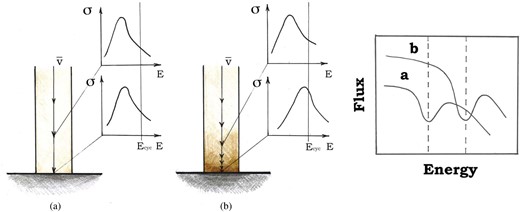
The schematic presentation of the dependence of the cyclotron line energy on the velocity profile in the line-forming region. The radiation pressure affects the velocity profile when the luminosity is approaching its critical value: the higher the luminosity, the lower the velocity in the vicinity of NS surface. The lower the electron velocity, the lower the redshift and the higher the resonant energy at a given height. As a result, a positive correlation between the line centroid energy and the luminosity is expected. Panel (a) corresponds to the low-luminosity case when the gas is in a free-fall. The observed cyclotron line is redshifted relative to the rest-frame value. Panel (b) is for the higher luminosity when the gas is decelerated close to the surface and the line shifts closer to the rest-frame position.
In this paper, we construct a simple model, which describes variations of the opacity near the cyclotron energy, and compare the predictions of our model with the observations obtained by the INTEGRAL space observatory of the XRP GX 304−1 during its type II outburst in the beginning of 2011.
2 THE MODEL
The basic process which determines the interaction between the radiation and matter in the vicinity of an NS surface is Compton scattering. In case of strong magnetic field, the scattering has a number of special features. Its cross-section strongly depends on the B-field strength, photon energy, polarization and momentum. Electron transitions between Landau levels cause the resonance scattering at some photon energies, where the cross-section can exceed the Thomson scattering cross-section by several orders of magnitude. The resonant scattering leads to appearance of cyclotron absorption features in the spectra of XRPs. The exact shape and position of the features in the spectra are determined by the structure of the line-forming region.
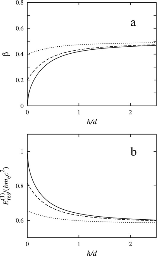
The dependence of (a) the dimensionless velocity and (b) the corresponding resonant scattering energy in the laboratory reference frame on the distance from the NS surface measured in units of the thickness of the accretion channel. The velocity profile is given by equations (6) and (7) and the cyclotron energy is computed from equation (1). Different curves correspond to various final electron velocities: β0 = 0 (solid), β0 = 0.2 (dashed), β0 = 0.4 (dotted). Here, the free-fall velocity is βff = 0.5 and the observing angle is θ = 0.
If the accreting matter is confined to a narrow wall of the magnetic funnel, the flux dependence on the height is more complicated. The flux drops as (1 + h2/d2)−1/2 when h ≪ l/(2π) and as (1 + 4π2 h2/l2)− 1 when h ≳ l/(2π), resulting in a slightly different velocity profile. However, the qualitative behaviour is the same (see also Lyubarskii & Syunyaev 1982; Becker 1998) and further in this paper we use equation (6) for calculation of the velocity profile.
Radiation from the hot NS surface has to pass through the layer of moving plasma and is resonantly scattered there by electrons. The resonant energy depends on the local electron velocity (see Fig. 2). As a result, it is expected that the position of the absorption line feature in the spectrum and its shape are determined by the plasma velocity profile near the NS surface. Higher luminosity would lead to lower velocity shifting the resonance to higher energy in the observer reference frame.
2.1 The opacity of moving plasma near the resonance energy
2.2 Opacity profiles
For our calculations we have taken an NS of mass M = 1.4 M⊙, radius R = 10 km and surface dipole magnetic field strength at the poles B0 = 5 × 10¹² G. The opacity averaged over the orientation of line-forming region (see equation 12) as a function of photon energy is presented in Fig. 3, where different lines correspond to different final velocity on the NS surface. The peak of the opacity, whose complicated shape is defined by the velocity distribution in the line-forming region, shifts to higher energies when the surface velocity of the accretion flow decreases. The lower the surface velocity, the wider the opacity peak produced by resonant scattering. The opacity profile determines the shape of the scattering feature in the XRP spectrum. Therefore, taking into account the connection between the accretion luminosity and the velocity β0, we find that the cyclotron absorption feature centroid energy and its width should be positively correlated with the luminosity for sub-critical XRPs: the higher the luminosity, the higher the line centroid energy, the wider the cyclotron line in the spectrum. The increase of the centroid energy is caused by the appearance of a layer with a lower velocity, where the redshift of the cyclotron energy is lower. This fact explains also the increase of the line width: it grows on its blue side because of the layers of lower velocity. We also note that the shape of the line is asymmetric and can hardly be approximated by the widely used Lorentzian or Gaussian profiles.
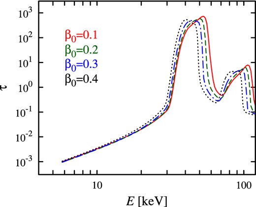
The averaged opacity profile for various final velocities β0 at the NS surface. The profiles are computed for the fixed accretion luminosity L = 1037 erg s− 1. We see that the lower the final velocity, the higher the centroid energy and the wider the feature. Here B0 = 5 × 10¹² G, i = 60°, α = 20°.
The behaviour of the line can be well illustrated by the ratio of opacities calculated for different surface velocity values (see Fig. 4). If one takes the ratio of the low-luminosity opacity (high β0) to the high-luminosity opacity (low β0), then the shape of the ratio is quite conservative and does not depend on the angles, which the opacity is averaged over: the ratio reaches a local maximum and then has a deep local minimum (see Fig. 4b). The same behaviour is expected for the ratio of higher luminosity XRP spectrum to the lower luminosity spectrum. Because we do not have a model for the spectrum formation, the analysis of spectral ratios can be suggested as a good test for the model.
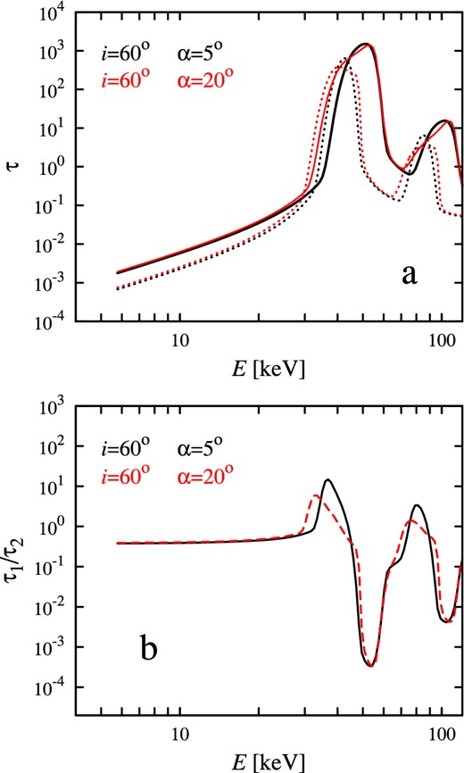
(a) The opacity profile averaged over the pulse period for various magnetic inclination α (see equation (12)). Black lines are for i = 60° and α = 5°, while red lines are for i = 60° and α = 20°. Solid and dotted lines are given for β0 = 0.1 and 0.4, respectively. (b) The ratio of the opacity profiles τ1 = τ(β0 = 0.4), τ2 = τ(β0 = 0.1) corresponding to the different velocities at the NS surface. Here B = 5 × 10¹² G.
It is also expected that the cyclotron line absorption feature has to show variability during the pulse period. The Doppler shift of the resonant energy is lower for larger angles between the accretion flow velocity and the line of sight (see equation 2). Therefore, it is expected that the phase-resolved line centroid energy would be anticorrelated with the pulse intensity for sub-critical XRP with a pencil beam emission diagram (Gnedin & Sunyaev 1973). Because the resonance peak in the scattering cross-section tends to be wider for the photons propagating along the B-field lines (Harding & Daugherty 1991; Mushtukov et al. 2015a), it is expected that the phase-resolved cyclotron line width would be positively correlated with the pulse intensity. The radiation beam pattern also affects the phase-averaged spectrum and its changes with the luminosity can affect the cyclotron line energy (Nishimura 2014). In our calculation the radiation beam pattern is taken into account in equation (10), where the opacity is weighted with the continuum intensity escaping in different direction.
3 COMPARISON WITH OBSERVATIONS
3.1 Observational data
The most reliable positive correlation between the cyclotron line energy and the luminosity has been observed in the spectra of XRP GX 304−1 (Yamamoto et al. 2011; Klochkov et al. 2012). Therefore, we use this source as a case study to verify the predictions of our model.
GX 304−1 belonging to the sub-class of XRPs with Be-type optical companions (Mason et al. 1978) has a relatively long pulse period of 272 s (McClintock et al. 1977). It is located at a distance of about 2.4 kpc (Parkes, Murdin & Mason 1980). The cyclotron absorption line at 54 keV in the source energy spectrum was discovered only recently (Yamamoto et al. 2011) using Suzaku and RXTE data obtained during type I outbursts recurrently observed from this system every 132.5 d.
In our current work, we reanalyse the data obtained by the INTEGRAL observatory (Winkler et al. 2003) during another type II outburst occurred in the beginning of 2011 (Yamamoto et al. 2012). The data sample is identical to the one utilized by Klochkov et al. (2012). The total duration of the outburst was about one month. It was evenly covered by eight INTEGRAL observations (during spacecraft revolutions 1131–1138). Both rising and declining parts as well as the maximum of the outburst were monitored.
The data from the IBIS/ISGRI detector (Lebrun et al. 2003) were screened and reduced following the procedures described in Krivonos et al. (2010) and Churazov et al. (2014). Energy calibration was provided by the Offline Scientific Analysis (osa) version 10.1 (Caballero et al. 2012). Additional gain correction based on the position of the tungsten fluorescent line (at 58.2 keV) was applied, keeping the uncertainty of energy reconstruction to less than 0.1 keV. Data from the JEM-X monitor (Lund et al. 2003) were processed with the standard procedures from osa 10.1.
Observed fluxes from GX 304−1 range between about 0.1 and 1 Crab, permitting us to trace the evolution of the energy spectrum in a wide energy range (5–100 keV) over very different luminosities of the source. Three spectra obtained at different states are shown in Fig. 5(a). Particularly, spectra obtained during the lowest luminosity state at the rising phase, peak phase, and lowest luminosity state at the declining phase of the outburst are denoted by Rev. 1131, Rev. 1134, and Rev. 1138, respectively. JEM-X data are used in the range 5–30 keV and shown by green and red circles (for JEM-X1 and JEM-X2 modules, correspondingly), IBIS/ISGRI data cover the energy range from 25 to 100 keV (shown by filled black circles). The solid curves represent the best-fitting models that consist of a power law with an exponential cutoff modified by the Gaussian line at 6.4 keV and the cyclotron absorption feature in the form of Lorentzian optical depth profile (CYCLABS model in xspec; Mihara et al. 1990). The final form of the fitting model in xspec package can be expressed as (GAU+POWERLAW*HIGHECUT)*CYCLABS.
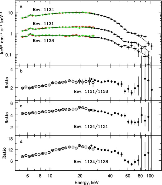
(a) Energy spectra of GX 304−1 obtained by main instruments of the INTEGRAL observatory during different spacecraft revolutions. Data in the energy range 5–30 keV are from JEM-X monitor (red and green points for JEM-X1 and JEM-X2 modules), between 25 and 100 keV – from the IBIS telescope. (b)–(d) Ratio of spectra obtained during different revolutions.
Three lower panels of Fig. 5 show the ratio of spectra obtained at different orbits (see Table 1). We see that the spectra during brighter states are harder. Such a behaviour can be accounted for by the increasing Compton y-parameter with increasing mass accretion rate (Postnov et al. 2015). The most important feature in all spectral ratios is a wave-like structure at energies between 40 and 80 keV. We see an excess and depression relative to the general trend below and above 55 keV, respectively.
Our results confirm conclusions made by Klochkov et al. (2012) about the positive correlation of the cyclotron energy with flux in GX 304−1. Dependence of the cyclotron line centre on the observed flux is shown in Fig. 6(a) for both shapes of the optical depth profile, Lorentzian (CYCLABS model; red points) and Gaussian (GABS model; blue points). The corresponding dependences of the line width on flux are shown in Fig. 6(b). We see that both the line energy and its width correlate with the flux. However, it is very important to keep in mind that the opacity profile differs significantly from a simple Gaussian or Lorentzian (see Section 2.2) at any intensity levels. These deviations leads to a difficulty with interpretation of the cyclotron energy obtained directly from the fits using such simple phenomenological models.
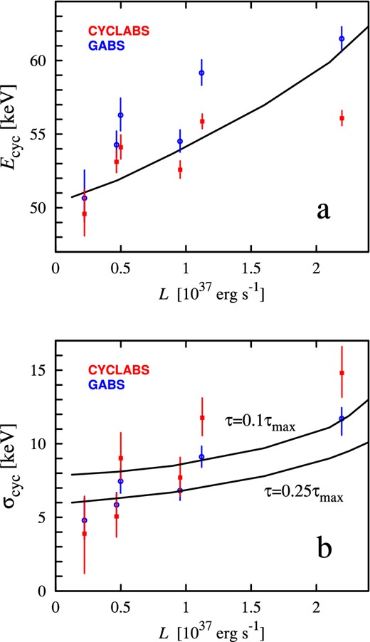
(a) The cyclotron line energy and (b) the cyclotron line width dependences on the 3–100 keV luminosity of GX 304−1. Red squares show results obtained using the Lorentzian profile of the optical depth (CYCLABS model); blue circles – using the Gaussian profile (GABS model) for the cyclotron absorption feature. Luminosities are calculated assuming the distance to the source of 2.4 kpc. Theoretical relations are given by black solid lines for the cyclotron energy at the NS surface for parameters Ecyc, 0 = 66.5 keV, i = 70°, α = 10°, L* = 2.7 × 1037 erg s− 1. A pure O-mode was considered. The width of the resonance is measured at the level of 10 and 25 per cent of the maximum τ(E).
3.2 Observations versus theory
Because there is no model of the line formation, we cannot predict well the shape of the absorption feature and its width. The line width in the observed spectrum can be different from the width of the resonance in optical thickness. We have measured the full width of the theoretical τ(E) dependence at the level of 10 and 25 per cent of the maximal τ as a function of the accretion luminosity (see black solid lines in Fig. 6b). We see that the model predicts a positive correlation, which is consistent qualitatively with the data. Moreover, we see that the observed ratios of the spectra obtained in different intensity states show very peculiar behaviour at the energies close to the cyclotron energy: the ratios reach local maximum below the cyclotron energy, then decrease and reach local minimum above the cyclotron energy (see Fig. 5). The same behaviour is seen in the ratios of the opacity profiles (see Figs 4b and 7) calculated for different velocity gradients and, therefore, different accretion luminosity. This observation is consistent with our model that the cyclotron line forms by scattering of the hard radiation from the hotspots of the electrons in the accretion flow and that the behaviour of the cyclotron line is determined by the changes of the velocity profile in the line-forming region.
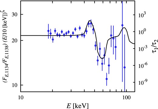
Ratio of spectra of GX 304−1 obtained in revolutions 1134–1138 corrected for different hardness ratio is given by blue circles (see also Fig. 5) and the ratio of the optical thicknesses for the case of pure O-mode polarization (solid line) for parameters Ecyc, 0 = 66.5 keV, ζ = 0.55, i = 70°, α = 10°.
Cyclotron line parameters for the INTEGRAL observations analysed in this work.
| Revolution | Lxa | CYCLABS | GABS | ||||
|---|---|---|---|---|---|---|---|
| number | (1037 erg s−1) | Ecyc | σcyc | τcyc | Ecyc | σcyc | τcyc |
| (keV) | (keV) | (keV) | (keV) | ||||
| 1131 | 0.50 | |$54.1^{+0.8}_{-0.8}$| | |$9.0^{+1.7}_{-1.5}$| | |$0.65^{+0.07}_{-0.07}$| | |$56.3^{+1.2}_{-1.1}$| | |$7.5^{+0.9}_{-0.8}$| | |$10.4^{+2.0}_{-1.8}$| |
| 1132 | 1.12 | |$55.9^{+0.5}_{-0.5}$| | |$11.8^{+1.3}_{-1.2}$| | |$0.74^{+0.05}_{-0.05}$| | |$59.2^{+0.9}_{-0.8}$| | |$9.1^{+0.7}_{-0.7}$| | |$14.3^{+2.1}_{-1.9}$| |
| 1134 | 2.20 | |$56.1^{+0.5}_{-0.5}$| | |$14.8^{+1.8}_{-1.6}$| | |$0.68^{+0.06}_{-0.05}$| | |$61.5^{+0.8}_{-0.7}$| | |$11.7^{+0.7}_{-1.1}$| | |$18.8^{+1.5}_{-1.2}$| |
| 1136 | 0.96 | |$52.6^{+0.6}_{-0.6}$| | |$7.7^{+1.4}_{-1.3}$| | |$0.53^{+0.05}_{-0.05}$| | |$54.5^{+0.8}_{-0.7}$| | |$6.8^{+0.7}_{-0.7}$| | |$7.5^{+1.3}_{-1.1}$| |
| 1137 | 0.47 | |$53.1^{+0.8}_{-0.7}$| | |$5.1^{+1.5}_{-1.4}$| | |$0.48^{+0.08}_{-0.07}$| | |$54.3^{+0.9}_{-0.9}$| | |$5.9^{+0.8}_{-0.8}$| | |$5.5^{+1.2}_{-1.0}$| |
| 1138 | 0.22 | |$49.6^{+1.6}_{-1.5}$| | |$3.9^{+2.5}_{-2.7}$| | |$0.39^{+0.56}_{-0.12}$| | |$50.6^{+1.9}_{-1.6}$| | |$4.8^{+1.5}_{-1.3}$| | |$3.8^{+1.7}_{-1.3}$| |
Note.aLuminosity in the 3–100 keV energy band, assuming source distance of 2.4 kpc.
In order to compare theoretical and observational wave-like structures, we use the ratio of spectra obtained at revolution numbers 1134 and 1138, when the accretion luminosities differ by a factor of 10, and correct the result for the difference in the spectral slope by multiplying it by the power-law Eζ with ζ = 0.55 (see Fig. 7). For calculation of the optical thickness ratio we used Ecyc, 0 = 66.5 keV and velocities on the bottom of line-forming region β0 = 0.1 and 0.4 for revolution numbers 1134 and 1138, respectively. During revolution 1134, the luminosity of GX 304−1 is very close to its critical value L* ≈ (2-3) × 1037 erg s− 1 (Mushtukov et al. 2015b), while during revolution number 1138 it is far below the critical luminosity. This fact explains our choice of β0 for the considered data sets (see also equation 8). The theoretical opacities were averaged over the pulse period with parameters i = 70° and α = 10° (see equation 12). We see that theoretical ratio of the opacities shows qualitatively similar wave-like structure seen in the data.
The cyclotron energy Ecyc, 0 = 66.5 keV is higher than line centroid energies measured from the data at any sub-critical luminosity states (see Fig. 6 and Table 1). This is well explained by our model: we always see a redshifted line absorption feature and only at critical luminosity the redshift (due to the Doppler effect) turns to zero, but the estimated line centroid energy might be still redshifted due to the complicated shape of the line. At sufficiently low-mass accretion rate corresponding to luminosities below 10−3L* even the resonant optical thickness drops below unity. At this point, the cyclotron line caused by scattering in the accretion flow disappears and the cyclotron line from the NS surface at E ≃ Ecyc, 0 can be observed in the spectrum. We thus expect that the positive correlation between the line centroid energy and the accretion luminosity discussed in the present paper should be replaced by a negative correlation at sufficiently low luminosities. Here we do not discuss the line formation in a region where the plasma flow is stopped by Coulomb collisions and assume that the initial spectrum does not contain scattering features. In that sense, the theory does not give a complete model for the line formation, however, it points at the effects that have to be taken into account and gives a qualitatively satisfactory description of the current observational data.
4 SUMMARY
We have shown that the cyclotron line absorption feature in the spectra of sub-critical XRPs can be produced by scattering off moving electrons in the accretion channel. The variation of the line position with the accretion luminosity is naturally explained by changes of the plasma velocity profile near the NS surface, which is affected by the radiation flux from the hotspot. The presented model has several characteristic features:
the line centroid energy is positively correlated with the luminosity,
the line centroid energy is always redshifted from the true cyclotron energy corresponding to the surface magnetic field at the NS pole,
the cyclotron line width is also positively correlated with the luminosity,
the line is expected to be asymmetric with excess at its red wing and it can hardly be approximated by widely used Lorentzian or Gaussian profiles,
the phase-resolved cyclotron line centroid energy and the width are expected to be negatively and positively correlated with the pulse intensity, respectively.
In order to get the exact shape of the cyclotron line, a self-consistent model of the line-forming region including radiation transfer and hydrodynamics is required, which is beyond the scope of this work. Our theory is shown to be in good qualitative agreement with the available observational data on the sub-critical XRP GX 304−1 and has profound implications for the interpretation of the data on the cyclotron lines observed in XRPs.
This work was supported by the University of Turku Collegium (SST), the Magnus Ehrnrooth Foundation (AAM), the Academy of Finland grant 268740 (JP) and the German research Foundation (DFG) grant WE 1312/48-1 (VFS). The authors are grateful to E. M. Churazov for developing the methods of analysis of INTEGRAL/IBIS data and providing the software. The research used the data obtained from the HEASARC Online Service provided by the NASA/GSFC.
REFERENCES
