


Abstract
We conduct a comprehensive numerical study of the orbital dependence of harassment on early-type dwarfs consisting of 168 different orbits within a realistic, Virgo-like cluster, varying in eccentricity and pericentre distance. We find harassment is only effective at stripping stars or truncating their stellar discs for orbits that enter deep into the cluster core. Comparing to the orbital distribution in cosmological simulations, we find that the majority of the orbits (more than three quarters) result in no stellar mass loss. We also study the effects on the radial profiles of the globular cluster systems of early-type dwarfs. We find these are significantly altered only if harassment is very strong. This suggests that perhaps most early-type dwarfs in clusters such as Virgo have not suffered any tidal stripping of stars or globular clusters due to harassment, as these components are safely embedded deep within their dark matter halo. We demonstrate that this result is actually consistent with an earlier study of harassment of dwarf galaxies, despite the apparent contradiction. Those few dwarf models that do suffer stellar stripping are found out to the virial radius of the cluster at redshift = 0, which mixes them in with less strongly harassed galaxies. However when placed on phase-space diagrams, strongly harassed galaxies are found offset to lower velocities compared to weakly harassed galaxies. This remains true in a cosmological simulation, even when haloes have a wide range of masses and concentrations. Thus phase-space diagrams may be a useful tool for determining the relative likelihood that galaxies have been strongly or weakly harassed.
1 INTRODUCTION
Early-type dwarf galaxies are easily the most common galaxies in clusters (Binggeli, Sandage & Tammann 1985). It is often stated that their low mass, and small potential well, should make them highly sensitive to their environment (e.g. Lisker et al. 2009). Environmental processes that could influence dwarf galaxies in clusters include ram-pressure stripping and starvation (Boselli et al. 2008), and harassment (Moore, Lake & Katz 1998) from high-speed tidal encounters with other cluster galaxies and the overall cluster potential. However, the significance of each mechanism for early-type dwarf galaxies is yet to be ascertained (see Recchi 2014 for a recent review of environmental effects).
Studies of dwarf ellipticals in Virgo – the nearest galaxy cluster – using the Sloan Digital Sky Survey optical imaging have revealed them to be an inhomogenous group of objects (Lisker, Grebel & Binggeli 2006; Lisker et al. 2007). Some are shaped like thick discs, and may contain prominent spiral arms or bars, or blue cores of central star formation. The degree of flattening is a function of luminosity, and the presence (or lack) of a nucleus (Lisker et al. 2009). Observations have also revealed that most early-type dwarfs are not morphologically simple (Aguerri et al. 2005; Janz et al. 2014); only approximately one-fifth are well described by a single Sérsic function with or without a nucleus. Roughly one third are found to have bars, and another approximately fifth have lens features (Janz et al. 2012; Janz et al. 2014). Dynamically, many early-type dwarfs are rotationally supported (Toloba et al. 2009). In fact rotating early-type dwarfs lie on the same Tully–Fisher relation as dwarf irregulars (van Zee, Skillman & Haynes 2004; Toloba et al. 2011). However, some early-type dwarfs have very complex dynamics including kinematically decoupled cores (Toloba et al. 2014a,b). Simulations demonstrate that harassment will rarely produce such features (González-García, Aguerri & Balcells 2005), supporting the idea that tidal encounters in a group environment may be required to reproduce the dynamics of those galaxies presenting these complex dynamics.
In this study we will focus on how harassment drives the evolution of dwarf galaxies in the galaxy cluster environment. Harassment is the combined effects of tidal forces from the overall cluster potential well, and repeated high-speed tidal encounters with other cluster galaxies. The effect of the high-speed tidal encounters can enhance mass loss and heating by ∼30 per cent (Gnedin 2003; Knebe et al. 2006). Tidal forces can strip dark matter, stars, and gas into low surface brightness streams that trail along the orbit of the galaxy through the cluster (Smith, Davies & Nelson 2010). Low surface brightness disc galaxies are especially sensitive to harassment and may have their stellar discs truncated and heated (Aguerri & González-García 2009), converting them into dispersion-supported objects that resemble early-type dwarfs (Moore et al. 1998). However high surface brightness giant discs are much more robust to harassment (Moore et al. 1999), losing only a small fraction of stars, and suffering some disc thickening (Gnedin 2003). Indeed, a difference in the size–luminosity relation of cluster discs compared to field discs is observationally detected. However, Maltby et al. (2010) find a size difference only in intermediate- and low-luminosity discs, whereas in Coma a size difference is also detected in massive discs (Aguerri et al. 2004; Gutiérrez et al. 2004).
Mastropietro et al. (2005) conducted simulations of harassment acting on stellar-only discy dwarfs in clusters, by placing high-resolution live models in a cosmological simulation of a cluster. Many of these initially thin, cool disc galaxy models ended up with thick, dispersion-supported stellar discs following harassment. A similar process of tidal stirring is also believed to have occurred to initially discy dwarfs in order to form the dwarf spheroidal population of the Milky Way (Mayer et al. 2006). However, the Mastropietro et al. (2005) simulations only explored a limited number of orbits which, unfortunately, do not constitute an unbiased subsample from the full distribution of orbits occurring during cluster assembly. As we will show later, this has important implications for assessing the impact of harassment in the evolution of low-mass satellites.
Harassment should also have an impact on the globular cluster systems (GCSs) of dwarfs in galaxy clusters. A population of luminous early-type dwarfs in clusters have very rich GCSs (Miller & Lotz 2007; Peng et al. 2008). Sánchez-Janssen & Aguerri (2012) argued that the richness and extent of their GCSs is evidence against their progenitors being brighter, more massive galaxies. They also showed that at a fixed stellar mass these massive early-type dwarfs also have a considerably larger globular cluster (GC) population than field dwarf irregulars, which also argues against a direct link between these two populations.1 One example is VCC 1087 which has >60 GCs (Beasley et al. 2006), and these are distributed out to 5–6 Reff. If the GCS is more extended compared to stars, then the GCs are expected to be even more sensitive to tidal stripping than the stars. Then tidal encounters can strip off GCs (Romanowsky et al. 2012), and potentially place the GCS briefly out of dynamical equilibrium, and/or modify their radial profile about a cluster galaxy. Interestingly, the GCSs of some early-type dwarfs (e.g. VCC 1087, VCC 1261, VCC 1528) appear highly rotationally supported (Beasley et al. 2009). In Smith et al. (2013c) we studied the impact of harassment on the dynamics of the GCSs of early-type dwarfs undergoing harassment using numerical simulations. We found that roughly ∼85 per cent of the dark matter haloes had to be stripped before we saw any removal of stars or globular clusters. This occurs because the stars and globular clusters are embedded deeply within the potential well of their galaxy's dark matter halo, and so are not tidally stripped until the dark matter halo is heavily truncated, and there is little dark matter left. Similar results are found for models of dwarf spheroidals suffering tidal stripping in the Local Group (Peñarrubia, Navarro & McConnachie 2008). New recipes could be developed, based on these results, for improving the modelling of stellar stripping from galaxies in semi-analytical models. Ryś, van de Ven & Falcón-Barroso (2014) claim that galaxies with higher dark-to-stellar mass ratio are preferentially found in the cluster outskirts, whereas central objects show ratios that are lower. Smith et al. (2013c) also studied whether the GCS dynamics were too disturbed by tidal encounters for dynamical masses, derived from their motions, to be useful. We found that the GCSs very quickly relax after a tidal encounter, and that unbound GCs quickly separate from the stellar body of the early-type dwarf. Therefore, the GCS dynamics provide good dynamical mass measurements, only failing when the early-type dwarf galaxy is on the verge of complete destruction (>95 per cent of the dark matter unbound).
However, Smith et al. (2010) found that the strength of the effects of harassment is highly dependent on the orbital parameters of the galaxy. This is in good agreement with fully cosmological simulations (Mastropietro et al. 2005). Eccentric orbits that pass near the cluster centre but have apocentre near the cluster virial radius were found to typically suffer weak effects from harassment. In comparison, a circular orbit near the cluster centre, that spends a much greater fraction of its time where the potential is most destructive, suffers strong mass loss from harassment. Bialas et al. (2015) also find that, in addition to orbit, disc inclination with respect to the orbital plane and disc size can also influence the amount of stellar mass lost. Smith et al. (2013c) found that most of the mass loss arises from the tides of the cluster potential, with a small additional amount of mass loss (∼30 per cent) due to high-speed tidal encounters with other cluster galaxies, in agreement with previous studies (Gnedin 2003; Knebe et al. 2006). Observationally, differences can be seen in the properties of cluster dwarfs if they are divided into two bins: high and low line-of-sight velocities. Those in the low-velocity bin are systematically more round in shape than those in the high-velocity bins, for a sample of galaxies at small projected distance from the cluster centre (Lisker et al. 2009). Muriel & Coenda (2014) show that for late-type galaxies between 1 and 2 virial radii from the cluster, a low-velocity sample showed systematically redder colour, higher surface brightness, and smaller size, at fixed stellar mass, compared to a high-velocity subsample.
Clearly, orbital parameters are highly important for dictating the strength of the cluster environmental effects. However, in Smith et al. (2010, 2013c) we considered only a limited range of orbits (e.g. circular near the cluster centre, or plunging from the cluster outskirts). Thus, the aim of this study is to carry out a comprehensive study of how orbital parameters control the strength of harassment. We therefore run simulations for 168 different orbits (each with their own unique orbital parameters) of an early-type dwarf galaxy model undergoing harassment in a simulated cluster environment. Our set up is described in Section 2, our results are given in Section 3, and we summarize and conclude in Section 4.
2 SETUP
2.1 The code
In this study we make use of gf (Williams & Nelson 2001; Williams 1998), which is a TREESPH algorithm that operates primarily using the techniques described in Hernquist & Katz (1989). The early-type dwarf galaxies we consider are gas-free and therefore not star-forming. We therefore do not include a smoothed particle hydrodynamics component or star formation recipe in our models, and so we operate the code purely as a gravitational code without considering hydrodynamics. gf has been parallelized to operate simultaneously on multiple processors to decrease simulation run-times. The tree code allows for rapid calculation of gravitational accelerations. In all simulations, the gravitational softening length, ϵ, is fixed for all particles at a value of 100 pc, which is large enough to avoid artificial clumping, and equal to the value used in the harassment simulations of Mastropietro et al. (2005). Gravitational accelerations are evaluated to quadrupole order, using an opening angle θc = 0.7. A second-order individual particle time-step scheme was utilized to improve efficiency following the methodology of Hernquist & Katz (1989). Each particle was assigned a time-step that is a power of two division of the simulation block time-step, with a minimum time-step of ∼0.5 yr. Assignment of time-steps for collisionless particles is controlled by the criteria of Katz (1991). For details of code testing, please refer to Williams (1998).
2.2 New harassment model
Following the approach of Smith et al. (2010), we model the dynamical and time-evolving potential of a galaxy cluster using analytical potentials (also see Knebe et al. 2005). An analytical gravitational potential is used for the main cluster, and each individual ‘harasser galaxy’ (cluster galaxies that can interact with a model galaxy) has its own unique analytical potential. This approach has advantages – the spatial resolution of gravity from harasser galaxies is effectively infinite. Also placing high-resolution model galaxies in cosmological simulations (e.g. Moore et al. 1999; Mastropietro et al. 2005) is numerically challenging. In comparison, computing accelerations from analytical potentials is very fast. There are also disadvantages, however, as harasser galaxies move on fixed tracks and cannot respond to the gravity of the live model galaxy. For high-velocity encounters this is of negligible consequence, but we are unable to accurately model low-speed tidal encounters using this approach and for this reason we deliberately select orbits resulting in high-speed encounters only (see Section 2.4 for more details).
In this study, we greatly improve on the harassment model of Smith et al. (2010, 2013c). In the new harassment model the properties of the main cluster halo and harasser galaxy haloes are dictated by a cosmological simulation of a cluster. We shall refer to the main cluster halo as the ‘cluster halo’ hereafter in order to distinguish it from other haloes. For each snapshot of the cosmological simulation we measure the properties (e.g. virial mass and radius) of all haloes at that instant. Then for each halo we construct an analytical potential that mimics each individual halo's tidal field. By applying the tidal field from all haloes simultaneously we construct the total tidal field of the cluster. Unlike in Smith et al. (2010) this approach allows for the growth in mass and structural evolution of the cluster with time as it accretes new galaxies. Furthermore, the properties of individual harasser galaxies also evolve in time.
The original cosmological N-body simulation was performed with an adaptive mesh refinement code mlapm (Knebe, Green & Binney 2001), and is fully described in Warnick & Knebe (2006) and Warnick, Knebe & Power (2008). Each dark matter particle has a mass ∼1.6 × 10⁸ h−1 M⊙, and the highest spatial resolution is ∼2 kpc. The cluster used is C3 from table 1 of Warnick & Knebe (2006). At z = 0 the cluster has a virial mass of 1.1 × 10¹⁴ h−1 M⊙, and a virial radius of 973 h−1kpc (a reasonable approximation to Virgo; see McLaughlin 1999 and Urban et al. 2011). The cluster is followed for ∼7 Gyr (since redshift = 0.8), during which time it approximately doubles in mass. A snapshot is produced once every ∼0.16 Gyr. This high time resolution enables us to follow the orbits of individual haloes with high accuracy. In any snapshot halo properties are measured with the halo finder MHF (MLAPM's halo finder; Gill, Knebe & Gibson 2004a), down to 20 particles per halo. Therefore, the minimum resolved halo mass is ∼3 × 10⁹ h−1 M⊙. There are initially a total of 402 haloes including the cluster and harasser haloes.
The properties and position of each halo in a snapshot are taken directly from the cosmological simulation using the Gill et al. (2004a) halo tracker. Between snapshots we linearly extrapolate halo positions and properties. As snapshots are only ∼0.16 Gyr apart this leads to smooth halo motion as a function of time. This procedure allows us to calculate the potential and accelerations at any position, and at any moment over the ∼7Gyr duration of the simulation.
By linearly extrapolating the position of each halo, halo velocities may be artificially reduced, especially near pericentre where the motion of the halo is least linear. We attempt to quantify the reduction in the orbital velocities using the following approach. We first calculate the orbit of a tracer particle in a host halo with the same mass and properties as the main cluster halo in our harassment model. We choose an orbit with orbital eccentricity of 0.8, and with pericentre distance (normalized by the cluster virial radius) of 0.2. As we will show in Fig. 10, this is a high-probability orbit in cosmological simulations of clusters. Because we choose a high eccentricity, low pericentre distance orbit, the effect of linear extrapolation should be relatively strong. We then measure the reduction in the true orbital velocity that would occur if we had used linear extrapolation between snapshots separated by 0.16 Myr, as done in our harassment model. We find the orbital velocity is reduced by no more than 4 per cent, and this only occurs when a halo is very close to pericentre where it spends little time. Therefore, we consider the linear extrapolation to have a negligible impact on our results.
2.3 Galaxy models
Our approach is to place live models of galaxies on orbits within the harassment model. Our galaxy models consist of three components: an NFW dark matter halo, a thick exponential distribution of stars, and a spheroidal distribution of globular cluster particles following a Hernquist profile.
2.3.1 The dark matter halo
Positions and velocities are assigned to the dark matter particles using the publically available algorithm mkhalo from the nemo repository (McMillan & Dehnen 2007). Dark matter haloes produced in this manner are evolved in isolation for 2.5 Gyr to test stability, and are found to be highly stable.
Our model galaxy has a dark matter halo mass of 1011 M⊙, consisting of 100 000 dark matter particles, with a concentration c = 14. The virial radius is r200 = 95 kpc with respect to the field. The peak circular velocity of the halo is 88 km s−1 at a radius of 15 kpc. If the halo were placed at a radius of 200 kpc within the smooth background potential of the cluster, the ratio of its central density is approximately five times that of the surrounding ambient medium.
2.3.2 The stellar distribution
The scalelength and mass of the stellar distribution are chosen to approximately match the observed properties of luminous Virgo dEs. These are characterized by close-to-exponential luminosity profiles (Janz & Lisker 2008). Our fiducial model has a total stellar mass of 3.0 × 10⁹ M⊙ (3 per cent of the halo mass; Peng et al. 2008), and is formed from 20 000 star particles. The stellar distribution has exponential scalelength Rd = 1.5kpc, consistent with the scalelength of disc galaxies of this stellar mass from Fathi et al. (2010). The effective radius is ∼2.6 kpc. The effective surface brightness of the model is ∼20 mag arcsec−2 in the H band, which is reasonable for early-type galaxies of this luminosity (Janz et al. 2014).
In the top panel of Fig. 1, we show the radial density profile of the dark matter halo (solid line), and the stellar distribution (dashed line). In the bottom panel of Fig. 1, the resulting circular velocity is shown (solid, dark blue line). This is similar to the circular velocity curves in observed early-type dwarfs (Ryś et al. 2014). We also show the azimuthal velocity (solid, light blue line), and the velocity dispersion components (dotted lines). A radially varying velocity dispersion is chosen that ensures the stellar distribution is Toomre stable (Toomre 1964) at all radii. In practice, a Toomre parameter of Q > 1.5 is required throughout the stellar body to ensure stability. We choose a fairly hot stellar system with a similar degree of rotational and dispersion support in the plane. Early-type dwarfs with a similar amount of dispersional support are observed in Virgo (Toloba et al. 2009; Toloba et al. 2011). This results in a thick stellar distribution with axial ratio b/a ∼0.6 consistent with the range of axial ratios observed in dwarf galaxies of this luminosity (Lisker et al. 2007; Sánchez-Janssen, Méndez-Abreu & Aguerri 2010). A full description of the procedures followed to set up the stellar distribution can be found in Smith et al. (2010).
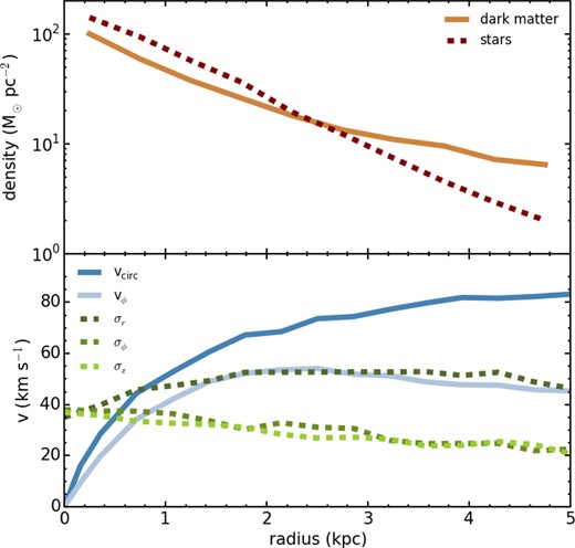
The radial density profile of the dark matter halo (solid line), and stellar distribution (dashed line), is shown in the top panel. These quantities are measured within annuli that lie parallel to the plane of the disc, and whose vertical height extends to ±1 kpc above and below the plane of the disc. In the lower panel, the circular velocity in the plane of the disc (solid, dark blue line) is shown, measured from the radial gradient of the potential. The azimuthal velocity (solid, light blue line) and the velocity dispersion components (dotted lines) are also shown, measured directly from the stellar dynamics.
We choose a thick, hot stellar disc for our dwarf galaxy, unlike in many previous harassment studies whose stellar discs are initially cold, thin and highly rotationally supported (e.g. Mastropietro et al. 2005; Smith et al. 2010; Bialas et al. 2015). The cool, thin discs of previous studies are often so thin that they have no known observable counterpart (Sánchez-Janssen et al. 2010). Harassment simulations that start with cool, thin dwarf discs demonstrate that to convert the thin discs into thick discs requires sufficient tidal heating that there is additional tidal stripping of the stars (e.g. see fig. 10 from Mastropietro et al. 2005). Our dwarf model approximates redshift zero observations of early-type dwarfs with thick stellar discs, and rich extended GCSs (e.g. VCC 1087). It is difficult to conceive how such dwarfs can initially have very thin discs, then lose enough mass that their stars are stripped and their discs thickened, without first stripping away their GCS (cf. Smith et al. 2013c). Therefore, it is likely that the types of galaxies we model formed with thick discs, or quickly evolved into thick discs through mechanisms other than heavy, harassment-induced tidal mass loss. Nevertheless, as we will discuss in Section 3.5.2, our choice of initially thick stellar discs has little significance for our key results on the amount of stellar stripping seen in our simulations. We will present a systematic study of stellar mass loss, and change in disc angular momentum, disc size, disc shape, and rotation-to-dispersion ratio, as a function of initial disc properties (e.g. disc thickness, disc size, halo profile, and initial rotation-to-dispersion ratio) in a follow-up publication.
2.3.3 The globular cluster distribution
The distribution is radially truncated at a cut-off radius of 7.5kpc. The observed GCS density distribution in luminous dEs depends on projected radius roughly as R−1 (Puzia et al. 2004; Beasley et al. 2006). We obtain an adequate match to this radial dependence by choosing the Hernquist scalelength rh = 3.75kpc (half the cut-off radius). Particle velocities are assigned using the Jeans equation for an isotropic dispersion-supported system.
Finally, we note that all models (combined dark matter halo, stellar distribution and surrounding GCs) are evolved in isolation for 2.5 Gyr to ensure stability, before introduction into the cluster environment model.
2.4 Orbits
We choose to fully simulate only orbits that match the following requirements.
Objects on first infall are excluded – galaxies must have had at least one pericentre passage.
Objects must have entered the virial radius of the cluster in the past.
Objects that entered the cluster in the past, but are now found out to twice the current virial radius are included – backsplash galaxies (see Gill, Knebe & Gibson 2005).
Objects that undergo low-speed tidal encounters are excluded – encounter velocities must be greater than 400 km s−1.
In practice, we find that galaxies that are on first infall do not result in any stripping of stars or globular clusters. In fact, as we will show, even those that have passed pericentre once show no mass loss of stars or globular clusters. Therefore, we choose to exclude ‘first-infaller’ orbits, as these consistently show no effects from harassment, and therefore we do not wish to spend computational time modelling systems where very little of interest occurs (requirement i). We also consider backsplash galaxies as these may have been affected by harassment when they were in the cluster, despite ending up outside of it (requirement iii). As discussed previously, harasser galaxies are on fixed orbital tracks and cannot respond to the potential of the live model. This is a reasonable approximation for a high-speed encounter, but is a poor description of a low-speed tidal encounter. Therefore, we choose to model only the high-speed tidal encounters of harassment, and exclude all orbits where low-speed tidal encounters occur (requirement iv). With encounter velocities >400 km s−1, we ensure collisions occur at greater than five times the internal velocities of the galaxy.
In order to find orbits that match these conditions, we place a massless tracer particle with the initial position and velocity of every halo in the cosmological simulation. We then evolve the orbits of all the massless tracer particles in the potential field of the harassment model. This step is necessary as the orbits of the massless tracer particles do not exactly match the orbits of the original dark matter haloes, as the analytical potentials used in the harassment model are only approximations to the potential field of the original cosmological simulation. However, by using massless tracer particles, we can quickly trace out all the orbits, and exclude those orbits that do not match our orbital criteria. We have confirmed that, when we replace a tracer particle with a live model of the galaxy, the tracer particle orbit accurately matches the orbit of the live model.
After filtering the orbits by these conditions, 168 out of 401 orbits remain. We simulate all of these with a live, high-resolution galaxy model. For each orbit we measure the most recent apocentre and pericentre distance, and then use these to calculate the orbital eccentricity of the most recent orbit e = (rapo − rperi)/(rapo + rperi).
2.5 Measured properties
2.5.1 Bound fractions
The following technique is found to be a reliable and reproducible method for measuring the fraction of particles that remain bound to the galaxy at any instant. Initially, the position of the centre of density is obtained. This involves finding the particle with the highest number of nearby neighbours. In practice, for each particle, the number of neighbours within a sphere is counted. The radius of the sphere is systematically varied from 0.1 to 1.0 kpc in nine equally spaced bins, and the position of the particle with the most neighbours is recorded for each of the nine bins. An iterative one-sigma clip is then applied to these nine positions, and the average of the positions that remain after the clipping is then used as the coordinates of the centre-of-density. Then in the next step all particles within a 2.5 kpc radius of the centre-of-density of the galaxy are selected. The choice of 2.5 kpc is fairly arbitrary, but is roughly of the order of the effective radius of the dwarf galaxy and the final bound fractions are found to be very insensitive to this choice of radius. Each particle confirms whether it is bound to the other particles within this radius. Those that are bound to each other are considered a bound core within the galaxy centre. Now an iterative procedure begins. In each iteration, all particles (including those beyond 2.5 kpc) are tested to see whether they are bound to the bound core. If they are, then their mass is added to the bound core. We call this method of growing the mass of the bound core the ‘snowballing’ method. Then the iteration is repeated until the bound mass of the galaxy increases by no more than 1 per cent between iterations. In practice, the total bound mass is found within five to 10 iterations. We find the snowballing method of measuring bound masses to be robust and trustworthy, and we have applied this technique successfully in several previous studies (Smith et al. 2013a,b,c).
2.5.2 Generalized Sérsic fits
3 RESULTS
3.1 Dependence of mass loss on orbital parameters
In Fig. 2, we show the residual bound mass fractions at redshift z = 0 (as symbol colour shading) as a function of the orbital properties of each galaxy model (i.e. eccentricity on the y-axis, normalized pericentre distance on the x-axis) for the dark matter (upper-left panel), stars (upper-right panel), and globular clusters (lower-left panel). In the lower-right panel, the symbol colour shading indicates the number of pericentre passages over the duration of each harassment simulation.
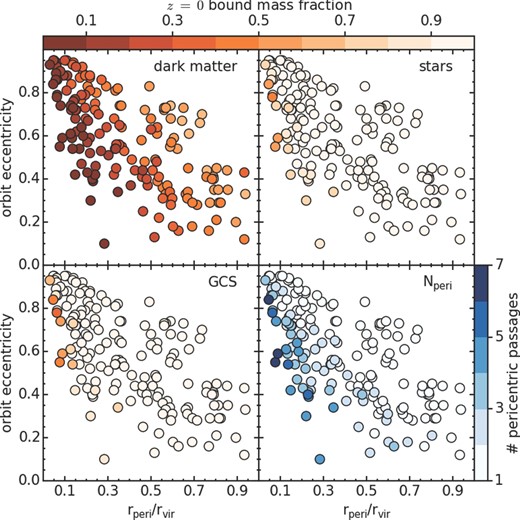
The effect of orbital parameters on the bound mass fractions of all 168 of our models. Colour of the symbol indicates the final bound mass fraction of the model's dark matter (upper-left), stars (upper-right), and globular clusters (lower-left), using the upper colour bar. In the lower-right panel, the symbol colour indicates the number of pericentre passages over the duration of the simulation (see lower-right colour bar). Each panel is a plot of the orbital parameters: eccentricity (y-axis) versus normalized pericentre distance (x-axis), where each symbol is one of our 168 galaxies.
3.1.1 Dependence of dark matter mass loss on orbit
This is shown in the upper-left panel of Fig. 2. The range of symbol colour shading across this figure indicates that dark matter mass loss depends strongly on orbital parameters. Small pericentre distances (to the left of the panel) tend to suffer greater dark matter mass loss. These destructive orbits can, however, have a wide range of eccentricity. Hence orbits with strong harassment fall in a tall and thin triangle, in the lower-left corner of the plot. If we classify strongly harassed galaxies as those that lose more than 85 per cent of their dark matter (see Section 3.1.2), the triangular shaped region reaches across to roughly rperi/rvir = 0.4, and up to eccentricities of almost 1. This wide range of eccentricity means that strongly harassed galaxies must have a large range of apocentres, indicating that such galaxies will not be found exclusively near the cluster centre.
To be as destructive as a circular orbit, a highly eccentric orbit must have a smaller pericentre distance – this is the reason the region of strong harassment is triangular shaped. We will show in Section 3.1.4 that the mass loss strongly depends on the pericentre distance and number of pericentre passages. There is a secondary dependence on eccentricity because, for a fixed pericentre distance, the eccentricity of the orbit will determine the number of pericentre passages. We note that here we have fixed the model galaxy's parameters and vary only the orbit. However, in Smith et al. (2013c) we found negligible change to the bound dark matter fraction when we varied halo mass by a factor of 10, and a modest ∼15 per cent change when we varied concentration from five up to 30.
3.1.2 Dependence of stellar and GCS mass loss on orbit
In the upper-right panel of Fig. 2 symbol colour indicates the final stellar bound mass fractions as a function of orbital parameters. Rather strikingly, the great majority of the orbits we consider result in no stellar mass loss at all. Only models which suffer the very strongest dark matter mass loss (>85 per cent unbound) show any stellar mass loss at all (those located in a tall, thin triangle in the lower-left of the distribution). This confirms our previous result that the stellar body only begins to be stripped once 80–90 per cent of the dark matter halo has been unbound (e.g. see fig. 5 of Smith et al. 2013c). This indicates that the stars are deeply embedded within the potential well of the halo, and so do not suffer tidal mass loss until the halo has been heavily truncated and stripped itself.
In the lower-left panel of Fig. 2 symbol colour indicates the final globular cluster bound mass fractions as a function of orbital parameters. In many ways the bound GCS fraction panel is roughly the same as the bound stellar mass-loss panel (upper-right panel), demonstrating that GCs and the stellar distribution are similarly affected by harassment. This is because the stars and GCs have a similar radial distribution. As we will show in Section 3.1.5, however, the GCSs actually suffer marginally more tidal mass loss. Nevertheless, most of the orbits considered result in no loss of GCs. Only when the strongest dark matter mass loss occurs (in the lower-left corner triangle described previously) are GCs stripped. Thus, tidal stripping of stars and globular clusters requires orbits with small pericentre distances, but orbital eccentricity can vary widely. Furthermore, for very high eccentricity orbits the pericentre distance must be very small to cause tidal stripping of the stars and globular clusters.
3.1.3 Mass loss as a function of specific energy and number of pericentre passages
As shown in the lower-right panel of Fig. 2 the great majority of our live models pass pericentre only once. This is because the cluster is constantly accreting new galaxies and so, at redshift zero, many galaxies may have only had time to be accreted and complete one pericentre passage. However, where dark matter mass loss was strong (in the lower-left corner triangle) galaxies suffer multiple pericentre passages (three to seven pericentre passages over the duration of the simulation). We further consider the correlation between number of pericentre passages and mass loss in the following subsections. Gill et al. (2004b) find that with increasing numbers of pericentre passages, the orbits of substructure in their clusters become more circularized, due to the growth in the depth of the potential well of their clusters with time. This suggests that those of our models with large numbers of pericentre passages had higher eccentricity in the past.
In Fig. 3 we consider the correlation between the final bound fraction of dark matter (red circles) and stars (blue triangles) as a function of orbital specific energy (left) and number of pericentre passages (right). Orbital specific energy (left) is calculated by the sum of the kinetic and potential energy of each galaxy, measured at redshift zero. There is a strong correlation between the amount of dark matter that is stripped and the orbital specific energy. Rocha, Peter & Bullock (2012) find that specific orbital energy is also positively correlated with time of infall into the host halo. There is also a clear correlation between the amount of dark matter and stars that are stripped and the number of pericentre passages the galaxy has completed by redshift zero (right panel). However, with each pericentre passage the fraction of the total bound mass that is stripped decreases rapidly. This is similar to the results of Taylor & Babul (2004), who find that with each pericentre passage between a quarter and half of the remaining bound mass of a subhalo is stripped.
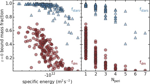
Correlations between the final bound fraction of dark matter (red circles) and stars (blue triangles) as a function of orbital specific energy (left; shown as log-scale) and number of pericentre passages (right).
3.1.4 Recipes for dark matter stripping as a function of orbital parameters
The time-averaged radius of an eccentric orbit can be expressed as ravg = (rperi,norm/(1 − e))(1 − e2), where rperi,norm is pericentric distance normalized by the cluster virial radius, and e is orbital eccentricity. In the left panel of Fig. 4 we plot final bound dark matter fraction versus time-averaged radius. As the time-averaged radius increases, the bound dark matter fraction increases. However, the trend broadens at larger radius due to eccentricity, with high eccentricity galaxies having relatively lower dark matter fractions. Therefore, the time-averaged radius alone cannot be used as a reliable predictor for the amount of mass loss suffered.
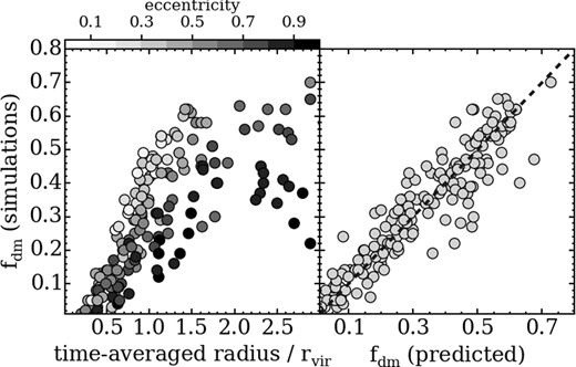
Final bound dark matter fraction versus time-averaged radius (left panel). Symbols are coloured by eccentricity (see colour bar). Final bound dark matter fraction versus predicted dark matter fraction (right panel) considering a simple mass-loss model where there is a constant fractional mass loss between each pericentre passage (see text for details).
In Taylor & Babul (2004), a simple recipe is considered for the mass loss of a satellite galaxy in a host halo. Between each pericentric passage, the mass of the satellite is found to decrease by between 25 and 45 per cent of its mass prior to pericentric passage. The exact fraction that is lost, which we will refer to as fperi, is found to depend on the halo's concentration, and the eccentricity of the orbit. If these parameters are fixed, the fraction of dark matter remaining after Nperi pericentre passages will be: fdm = (1 − fperi)|$^{N_{\rm {peri}}}$|. For our models, we know fdm and Nperi (upper-left and lower-right panel of Fig. 2, respectively), so we can calculate fperi, in eccentricity and pericentre space.
In practice, we find there is no clear trend in fperi with eccentricity, when pericentric distance is fixed. The lack of a trend with eccentricity may arise because, with each pericentre passage, a galaxy's orbit becomes increasingly circularized by growth of the cluster potential (Gill et al. 2004b). Instead, we find a clearer trend with pericentric distance. The trend has a linear form and can be approximated by fperi = 0.70 − 0.43 rperi,norm. Therefore, the mass lost at each pericentre can vary from 27 per cent (at rperi,norm=1.0) up to 70 per cent (at rperi,norm=0.0). Our upper limit of fperi=70 per cent is higher than the 45 per cent of Taylor & Babul (2004). However, their recipe was for a satellite orbiting in a single host halo, and thus additional mass loss from harassment was not considered.
Using this recipe, if we consider a galaxy with normalized pericentric distance rperi,norm, we can calculate fperi. Then, if the galaxy has Nperi pericentre passages, we can predict the final dark matter fraction. In the right-hand panel of Fig. 4, we show the correlation between the predicted and the real dark matter fraction. A good correlation can be seen, and the predicted dark matter fractions matches the real dark matter fractions to within ±0.11 (one-sigma errors).
In summary, a simple description for the distribution of dark matter mass loss in orbital parameter space can be found if we follow the approach of Taylor & Babul (2004). For a given orbit, we assume a constant fraction of the dark matter is lost between each subsequent pericentric passage. We find that this constant is a linear function of the pericentric distance of the orbit. In this description, with increasing numbers of pericentre passages, a galaxy suffers increasing amounts of mass loss. The number of pericentre passages is a function of both pericentre distance and eccentricity (e.g. see lower-right panel of Fig. 2). In this way, the total mass loss becomes a function of both pericentre and eccentricity, although the fractional mass loss between pericentre passages is only a function of pericentre distance. With further testing, this recipe for dark matter stripping may be useful for semi-analytic models of galaxy formation where dark matter stripping is often prescribed based on simplistic simulations of dark halo interactions (e.g. Lee & Yi 2013). We will test this prescription thoroughly in a future study, using cosmological simulations of clusters and groups with a wide range of masses.
3.1.5 Histograms of mass loss
In Fig. 5 we show the bound mass fractions by z = 0 for all our sample of model galaxies. At z = 0, all our haloes have lost at least ∼30 per cent of their dark matter (brown). There are of roughly equal numbers in each bound mass bin between a bound mass fraction of 0.0 (all dark matter stripped), and 0.6 (only 40 per cent of dark matter stripped). In comparison, the stars (blue) and globular clusters (green) suffer weaker fractional mass loss – there are few models (∼5 per cent) that lose more than ∼20 per cent of their stars and globular clusters. This is because the stars and globular clusters are deeply embedded within the dark matter halo. Therefore, the halo must be heavily truncated and stripped for the stars and globular clusters to suffer tidal stripping. In fact, it can be seen that the globular clusters are slightly more susceptible to tidal stripping than the stars. This is because in our initial conditions we assume the globular cluster distribution is slightly more radially extended than the stars. Wetzel & White (2010) classify galaxies that have lost ≥97 per cent of their dark matter as destroyed in their semi-analytical model prescription. Only seven of our 168 models lose this much dark matter, and they lose 25–59 per cent of their stars, and 28–68 per cent of their GCS. However, we note that the distribution of orbits found in our harassment simulations should not be considered identical to that found in cosmological simulations. Therefore, to quantify the number of orbits that result in strong mass loss, we instead consider the fraction of such orbits found in cosmological simulations (see Section 3.5.1).
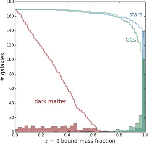
The bound mass fractions at z = 0 for all our model galaxies. Shaded histograms indicate the number distribution. Stepped lines indicate the cumulative distribution, which is cumulative moving from the right to the left. Colour indicates bound fractions of dark matter (brown), stars (blue), and globular clusters (green).
3.2 Final radial profiles of stars and the GCS – dependence on orbit
3.2.1 Effects on scalelengths of stars and the GCS
In each panel of Fig. 6, symbol position shows the orbital parameters of each model, as in Fig. 2. We see that much of the orbital parameter space results in a stellar distribution that is entirely unaffected by harassment. Those stellar bodies that lose no stars are also unchanged in effective radius. In the case of the strongest harassment, when stars are stripped, our models show reduced effective radii as their stellar distributions are truncated.
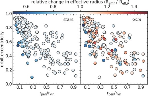
Effect of orbital parameters on the scalelength of the spatial distribution of the stars (left panel) and globular clusters (right panel). Each panel is a plot of the eccentricity (y-axis) versus normalized pericentre distance (x-axis), where each symbol is a single galaxy from the harassment simulations. Symbol colour indicates the change in the effective radius.
In the right panel symbol colour indicates the exponential scalelength of the GCS distribution. Comparing to the stellar effective radius (left panel), the exponential scalelength of the GCS is less clearly correlated with orbit. There is a weak hint that the smallest scalelengths are found preferentially to the left of the distribution of points. However, in general the trend with orbit is very noisy due to the fact that, with only a few dozen globular clusters, we suffer low-number statistics when measuring the GCS scalelength. Also, by measuring variations of the inner GCS, we are probing changes in the innermost radii of the GCS, instead of the outer GCS which is more sensitive to harassment. We find clearer results by studying averaged number density profiles, as shown in Section 3.2.2.
We measure a projected number density profile of the GCS for each model galaxy by placing a series of circular annuli, centred on the centre-of-density of the stellar distribution. We then average the profiles for certain subsamples and illustrate the results in Fig. 7. The blue lines are the whole sample, the green and red lines are for a sub-sample of strongly harassed (fdm < 0.1) and very strongly harassed (fdm < 0.05) galaxies, respectively. Error bars indicate the standard deviation. Between the panel rows we vary how extended the GCS is initially. The middle row is our standard model with a Hernquist scalelength rh = 3.75 kpc. In the upper row we halve the initial scalelength creating a concentrated GCS (‘conc GCS’) model, and in the lower row we double the initial scalelength creating an extended GCS (‘extd GCS’) model.

Projected GC surface density profiles, averaged for all galaxies (blue curves), a sub-sample of strongly harassed galaxies (green curves) and very strongly harassed galaxies (red curves). Error bars indicate the standard deviation. The left column panels are the projected number density as a function of radius. The right-column panels show the projected number density as a function of galactocentric radius normalized by the effective radius of the stellar distribution. The distributions for three types of GCS concentrations are shown. The middle-row panels illustrate the results for the standard model used in this study, whereas the upper-row panels show the corresponding relations for an identical model except, in the initial conditions, the scalelength of the GCS distribution is halved creating a concentrated distribution. Similarly in the lower-row panels, the curves show the results when the scalelength of the standard model is doubled creating an extended GCS distribution.
3.2.2 Effect on the GC-averaged number density profile
We first consider our standard model – see the central-left panel. Even for strong harassment we find only a weak change in the GCS profile (compare the blue and green lines). However, if harassment is very strong a significant change occurs, with the profile steepening at small radius, and flattening at large radius. Could this be used as a test of the strength of harassment in real galaxies? Unlike the model galaxy, real galaxies have a range of initial sizes. Therefore, to create an average profile it is necessary to normalize the radius by the effective radius of the stars in the galaxy, as shown in the centre-right panel. The effective radius is measured at the same instant that the GCS is viewed. Unfortunately, now the difference between the red and blue line is not so strong. This is because for very strong harassment, both the stellar disc and GCS are being affected by harassment in a similar way. When the GCS changes shape the effective radius is reduced, and this causes the change in profile shape to be less prominent when the normalized radius is used.
This is not the case if the stars and GCS are affected to differing degrees by harassment. For example, compare the middle-right panel to the upper-right and lower-right panels. If the GCS is initially very extended, it is preferentially truncated by harassment with respect to the stars, and then a change due to harassment is visible, even when the radius is normalized by the effective radius. Alternatively, if the GCS is initially very concentrated, then it is the stars that are preferentially truncated by harassment, while the GCS is nearly unaffected (see upper-left panel). Thus when the radius is normalized by the effective radius, the GCS appears to become more extended as a result of harassment.
The conclusion to draw from this is that the GCS profile is indeed altered when there is very strong harassment, at least in the standard and extended GCS case. However, when normalized radius plots are used, as is necessary for a real galaxy sample, detecting the change in profile becomes an additional function of how extended the GCS initially was with respect to the stars. If the GCS is initially very extended (considerably more than is currently observed) compared to the stars, then it is more sensitive to harassment than the stars. Then a change in GCS profile could be detected in the case of very strong harassment.
3.3 Changes to the circular velocity profile
We calculate the total mass profile, measured in a spherical volume, as a function of radius for all of our galaxies at z = 0. The total mass profile is converted into a circular velocity profile for each galaxy. We separate our galaxies into subsamples based on their final bound dark matter fraction, and combine the profiles together in each subsample to calculate an average circular velocity profile. The results are shown in Fig. 8. The key indicates the range of bound dark matter fraction for each subsample. At large radius (r ∼ 10 reff), the circular velocity is most sensitive to the mass loss, indicating preferential stripping of the outer halo first. Comparing the blue curve to the orange curve, we see that even when 80–95 per cent of the dark matter is stripped (orange curve), the mean circular velocity has only fallen by ∼20 per cent at 5 reff. This indicates that the majority of the dark matter losses occurred beyond 5 reff. However, if we consider the innermost circular velocity profile, there is very little change. This demonstrates that the innermost dark matter has been affected only weakly. A more significant change occurs to the circular velocity profile if harassment is very strong [i.e. resulting in more than 95 per cent loss of dark matter (red curve)]. Now the mean velocity profile falls by ∼45 per cent at 5 reff, and the gradient of the profile at small radii begins to flatten. Although we note that, even with such strong harassment, the mean circular velocity in the inner 0.5 reff is still only slightly reduced.
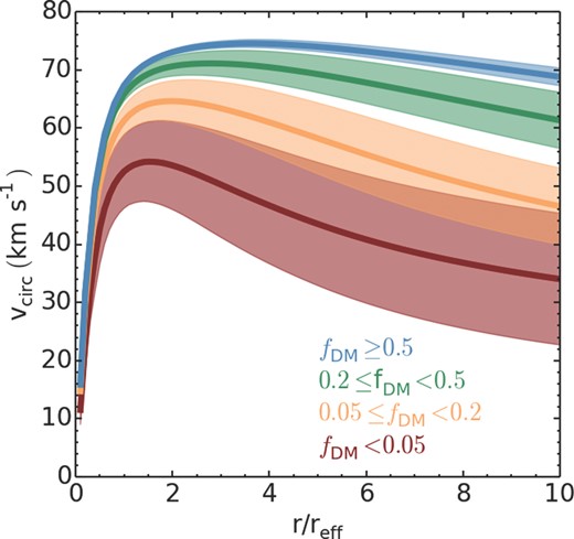
The averaged circular velocity profile of our model dwarf galaxies, separated into subsamples according to the strength of dark matter mass loss that occurred due to harassment (see legend). fdm > 0.5 can be considered weak harassment with no stellar stripping (blue curve). fdm < 0.05 can be considered very strong harassment resulting in significant stellar stripping (red curve). Shading indicates the one-sigma deviation of the subsample from the mean value.
3.4 Mass loss within one effective radius
In Fig. 9 we plot the ratio of the total mass over the stellar mass (Mtot/M⋆) within one effective radius as a function of a galaxy's normalized clustocentric radius. All quantities are measured at z = 0 for all our galaxy models (grey symbols). At large radius (R > 1.5 Rvir) the ratio approaches ∼2.2, which is the value of our initial conditions. With decreasing radius the ratio falls in value to Mtot/Mstr ∼ 1.6, with some scatter (values from ∼1.4 to 2.2). In general, our simulations show only a mild decrease in Mtot/Mstr as we move to smaller clustocentric radius. The gradient is shallow because mass is lost preferentially beyond one effective radius in our models (see the previous section). These results can be compared with the data points of observed early-type dwarfs from fig. 8 of Penny et al. (2015), given the caveat that the observed early-type dwarfs may not be subject to the constraint of having conducted at least one pericentre passage, as are our model dwarfs. We overlay the observed data points (orange symbols) on our plot. In general, the trend between the observed galaxies and our simulations is similar. However there is clearly significantly less scatter in the simulation results compared to the observations. Although this is to be expected given that we use exactly the same model dwarf galaxy for each harassment simulation. Also, our results are measured directly from the simulation and so do not have measurement errors. Meanwhile, the real dwarfs may have an intrinsic scatter in their properties, even prior to the effects of harassment. In addition, there is scatter due to measurement errors in Mtot/Mstr. These measurement errors are typically greater than ±0.5 (e.g. Ryś et al. 2014; Penny et al. 2015).
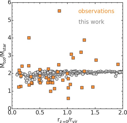
The ratio of the total mass over the stellar mass, measured within one effective radius, is plotted against the normalized clustocentric radius for our model galaxies (grey symbols). All quantities are measured at z = 0. The grey line indicates the running mean of our data points. Orange symbols indicate the observed results, compiled from several sources, by Penny et al. (2015).
3.5 Searching for strongly harassed galaxies
3.5.1 How many are strongly harassed?
We have previously seen that ‘strong harassment’ (i.e. harassment sufficiently strong to cause at least some stripping of stars and globular clusters) only occurs in a tall triangle in the lower-left corner of the eccentricity–pericentre distance plots (e.g. see upper-right panel of Fig. 2). Therefore, strong harassment occurs preferentially for orbits with small pericentre distance, but can have a range of eccentricity (hence the triangle extends up to eccentricity ∼1.0). To get an approximate estimate of the fraction of galaxies that fall within the ‘strong harassment’ area of the orbital parameter space, we return to the eight cosmological clusters described in Warnick & Knebe (2006). All eight clusters have similar, Virgo cluster-like masses [∼(1–3) × 1014 M⊙].
We first define a region in the orbital parameter space in which we see strong harassment occurring. This is simply done by eye, based on where we see stripping of stars, truncation of the stellar distribution, and unbinding of GCs (i.e. from the upper-right, lower-left panel of Fig. 2, and left-panel of Fig. 6). Clearly, doing this by-eye is rather approximate, but we only wish to get a rough estimate of the fractions of haloes in cosmological simulations with these types of destructive orbits. We choose a line that intersects the y-axis at an eccentricity of 1.0, and intersects the x-axis at rperi/rvir = 0.4, and every point below this line is assumed to lie in the strong harassment area. For every halo in the cosmological simulations, we measure the eccentricity and pericentre distance of the most recent orbit.
Fig. 10 shows the distribution of orbital parameters from the cosmological clusters. We exclude ‘first-infaller’ orbits in order to compare with our harassment models. The darkness of the blue shading indicates the relative numbers of haloes that fall in any one pixel. The dark blue region indicates that orbits with eccentricities of ∼0.6–1.0 and pericentre distance of ∼0.0–0.2 are relatively more common than other orbits in our cosmological clusters. This is in good agreement with the eccentricity and pericentre distributions in other cosmological simulations (Benson 2005; Wetzel 2011). The halo finder used (see Gill et al. 2004a) tracks haloes even after they have been destroyed. Therefore, the lack of orbits in the lower-left corner of Fig. 10 indicates that such orbits are genuinely rare. However, the lack of orbits in the upper-right corner is due to the fact that we only consider orbits that conduct at least one pericentre passage, and there is not enough time for objects with such orbits to fall into the cluster.
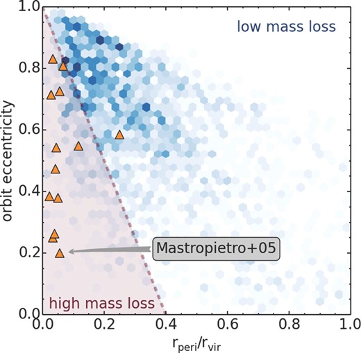
Relative probabilities of different orbital parameters (eccentricity on the y-axis, normalized pericentre distance on the x-axis). Darker pixel indicates orbital parameters that are more commonly found in the eight cosmological cluster simulations from Warnick & Knebe (2006). All haloes that were on first infall are excluded from this plot in order to make it comparable to these harassment simulations. The shaded region beneath the dashed line indicates the region of orbital parameter space where we see sufficiently strong harassment to begin stripping the stellar body of the galaxy in our harassment models (e.g. see upper-right panel of Fig. 2). Orange triangles indicate the orbital parameters for the 13 galaxies from Mastropietro et al. (2005) that have experienced at least one full orbit.
We calculate the total percentage of haloes that fall within the ‘high mass loss’ area shown in Fig. 10. If we consider haloes that are found out to two virial radii at redshift zero (i.e. including the backsplash population) we find 19 per cent lie in the triangle of orbits where at least some stars were stripped (i.e. the final bound stellar fraction is less than one). If we consider just the C3 cluster in the same way (which is the cluster we have used for the harassment model) the percentage is 18 per cent indicating that cluster–cluster variations are not large. Once again we consider all the clusters together, but this time we include only haloes found within one virial radius at redshift zero (i.e. excluding the back-splash galaxies). The percentage in the triangle is now 25 per cent, and therefore it is reasonable to state that less than a quarter of the orbits we measure in our cosmological simulations would result in stellar stripping.
In any case, the great majority of haloes in our cosmological simulations do not have orbits which result in strong harassment. As all our clusters are roughly the mass of Virgo-like clusters, we suggest that this may be true for early-type dwarfs in Virgo too. In other words, the majority of early-type dwarfs in Virgo may have only suffered weak harassment (with no stellar stripping, or change in disc size) despite spending many gigayears in the cluster environment. We note that if we had included first infallers, the percentage of orbits resulting in strong harassment would likely be even lower, strengthening our conclusion even further. One caveat, however, is that we have assumed dwarf galaxies initially have thick, dispersion-supported stellar discs. A second caveat is that we assume they enter the cluster environment as initially unperturbed systems, whose mass is dominated by an extended dark matter halo, in common with previous harassment studies, and consistent with the results from halo abundance matching (Guo et al. 2010).
3.5.2 Comparison with Mastropietro et al. (2005)
The small fraction of strongly harassed dwarf galaxies we find appears to be strongly at odds with the results of Mastropietro et al. (2005), which claimed that harassment was highly efficient at stripping and heating stars from their model dwarf galaxies. In this section we attempt to understand the source of these apparent differences.
First note that, by construction, the 20 orbits simulated by Mastropietro et al. (2005) do not represent an unbiased subsample of the underlying orbital distribution for cluster haloes. On the contrary, half of their orbits correspond to particles that were already within the virial radius by z = 0.5 and, more importantly, the other half were located within 0.2 rvir at that time. As a result, their initial distribution of orbits is biased towards orbits that result in strong harassment. This is shown by the orange triangles in Fig. 10, where we plot all 13 galaxies from their simulations that have completed at least one orbit about the cluster by z = 0 on to our probability density distribution of orbits (blue shading). It is clear that most of the galaxies have rperi/rvir < 0.1 (with the exception of two galaxies). Furthermore, all but one fall within the triangle where we find harassment is sufficiently strong to affect the stellar discs of our model galaxies. Therefore, it is perhaps unsurprising that for those 13 systems they find harassment to be highly influential for the stellar component of galaxies. If we were to randomly select orbits from our cosmological simulations, it is highly unlikely that we would choose so many orbits falling within this triangle. This can be seen by comparing the location of the Mastropietro et al. (2005) data points to the distribution of orbits in our cosmological simulations. In fact, in the previous section we found that less than ∼20 per cent of all subhalo orbits fall within this triangle, whereas this fraction is ∼60 per cent in the Mastropietro et al. (2005) simulations.
Secondly, one might wonder how well our results compare to Mastropietro's for galaxies on similar orbits about the cluster. In Fig. 11 the shading of each symbol indicates the amount of bound dark matter. Moving across the figure from lower-left to upper-right, bound dark matter fractions increase both in our simulations (circle symbols) and in those from Mastropietro et al. (2005) (triangle symbols) in a similar manner. For similar types of orbits, the amount of dark matter remaining in our models is comparable with the amount of dark matter remaining in the Mastropietro et al. (2005) simulations. Thus, our model dwarf galaxies are responding in a similar manner to the Mastropietro et al. (2005) dwarf models when they have similar orbits.
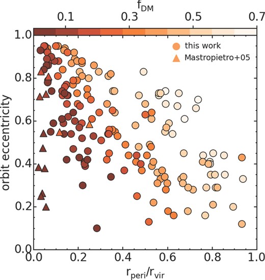
Comparison of the dark matter bound fractions from our simulations (circle symbols) with the 13 galaxies available from Mastropietro et al. (2005; triangle symbols). Symbol shading indicates the remaining bound dark matter fraction, with darker shading showing lower remaining bound dark matter fractions (i.e. stronger mass loss).
One clear difference between our initial conditions and those of Mastropietro et al. (2005) is that we choose a stellar disc that is thick, hot, and dispersion dominated, whereas their galaxy stellar discs are initially thin, cold, and rotation dominated. However, this does not cause a significant change in the amount of tidal stripping of stars. For example, their thin cool discs do not lose significant numbers of stars (>10 per cent) until large amounts of dark matter (>85 per cent) have been stripped. This is almost identical to what is seen in our models (e.g. see fig. 5 from Smith et al. 2013c). Therefore, disc thickness and the amount of dispersion support are apparently not sensitive parameters controlling stellar mass loss in early-type dwarf discs. In addition, Kazantzidis et al. (2011) find that tidal transformation of discy dwarf galaxies into dSphs occurs essentially independent of disc thickness.
Finally, it is important to point out that the seven (out of 20) galaxies in Mastropietro et al. (2005) that have not completed one full orbit about the cluster by z = 0 barely lose any stellar mass, and their discs suffer very little thickening or morphological transformation (other than the development of a bar; see table 1 and fig. 10 in that paper). Unfortunately, these objects receive little attention throughout the subsequent analysis and discussion, giving the impression that the majority of cluster galaxies are strongly influenced by harassment.
In summary, we show that our model dwarfs suffer similar amounts of mass loss of dark matter as those considered in Mastropietro et al. (2005) if they have similar orbits. However, harassment appears much more influential in Mastropietro et al. (2005) as the type of orbits they consider are biased towards orbits that result in strong mass loss. Furthermore, the majority of their models that suffer no stellar mass loss are neglected from the main body of their analysis. We find that changes in orbit can be very significant for the strength of harassment. This highlights the importance of considering the statistical probability of particular orbits when interpreting the results of harassment simulations, especially when a limited number of orbit types are considered.
3.5.3 Where are the strongly harassed galaxies found now?
In Section 3.5.1, we find that the strongly harassed dwarf galaxies are probably not found in substantial numbers in clusters. However, where might we expect to find the small fraction that are strongly harassed? We have previously seen that strong harassment occurs primarily for orbits with small pericentres (e.g. see upper-left panel of Fig. 2). However strong harassment orbits can have a broad range of eccentricities meaning their apocentres can be spread beyond the cluster core. Furthermore, galaxies with eccentric orbits spend the majority of their time at apocentre, and therefore it is inevitable that strongly harassed galaxies will be found beyond the cluster core. Consider the triangular area of ‘strong harassment’ we defined in Section 3.5.1. If we calculate the apocentre of orbits that fall on the hypotenuse of this triangle, we find a range of normalized apocentre of rapo/rvir = 0.4-0.8. Thus, we expect that strongly harassed galaxies may be found almost out to the virial radius of the cluster.
We confirm this in Fig. 12, where we plot the final dark matter fraction fdm as a function of the final clustocentric radius (normalized by virial radius) for all our harassment models. There is a clear, strong trend for decreasing bound dark matter fraction with decreasing distance to the cluster centre. However, the trend is very broad, meaning that a wide range of dark matter bound fractions may be found at any particular radius. For example, at the virial radius, galaxies can be found with bound fractions less than 0.1 or greater than 0.7. The most eccentric orbits (those with symbols that are more blue) are preferentially (but not uniquely) found lower in the spread. This can be more clearly seen by comparing the running averages of low (red) and high (blue) eccentricity galaxies. This occurs because galaxies spend a significant fraction of their time near apocentre. Given a group of objects at a particular radius that are all simultaneously at apocentre, those that have more eccentric orbits are able to pass closer to the cluster centre when at pericentre, and this is where the tidal field is more destructive. It is also interesting to note that galaxies with fdm < 0.1 (i.e. strongly harassed galaxies) can be seen at a large range or radii, out to near the virial radius of the cluster. This means that we cannot assume that strongly harassed galaxies are only found near the cluster centre, and thus determining if a galaxy is strongly harassed based on the clustocentic radius alone is very difficult.
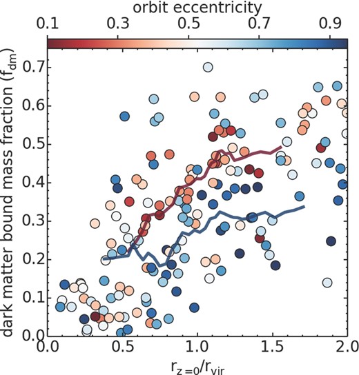
Bound dark matter fraction versus (normalized) clustocentric radius from the final snapshot of this study's harassment simulations. Symbol colour indicates the eccentricity of the orbit (see colour bar). The blue curve is a running average of data points with eccentricities >0.75, while the red curve is a running average of data points with eccentricities <0.3. There is typically an offset between the red and blue curve indicating that, at fixed radius, galaxies that have suffered the most mass loss are typically on more eccentric orbits. This occurs because eccentric orbits can bring more plunging, and so more tidally stripped galaxies out to apocentre where they spend the majority of their time.
However we can make progress if we consider the orbital velocity of the galaxy and simultaneously the clustocentric radius. A diagram of orbital velocity versus clustocentric radius is known as a ‘phase-space diagram’. In the upper panel of Fig. 13 we show the phase-space diagram of our harassed model galaxies in the final snapshot. Galaxy orbital velocities tend to rise as the clustocentric radius becomes smaller, as expected for galaxies that fall into the potential well of the cluster and gain velocity as a result. Symbol shading indicates the remaining bound dark matter fraction, with darker symbols having suffered more mass loss. At a fixed radius, the models which lose more dark matter are systematically at lower orbital velocity. This is likely due to the growth in mass, and so deepening of the potential well, of the cluster with time. Thus galaxies that fall into the cluster in the past tend to have lower velocities than galaxies that infall more recently. As a result, galaxies which have spent more time being affected by the cluster also have lower velocities, and so are offset in phase-space.
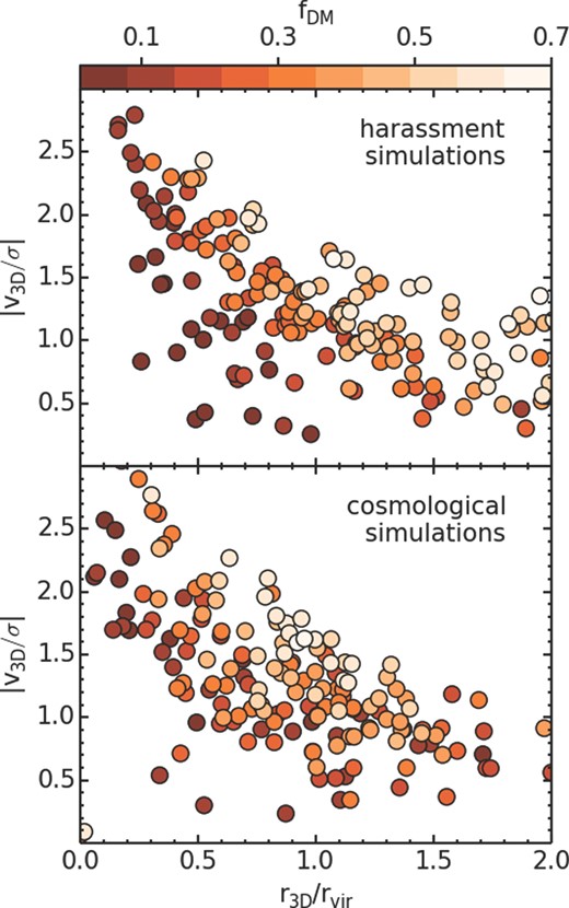
Phase-space diagrams of haloes in the final snapshot from our harassment model galaxies (top panel), and from the cosmological simulation of the C3 cluster of Warnick & Knebe (2006) (lower panel) where we exclude first infallers. The three-dimensional orbital velocities (y-axis) are normalized by the 3D velocity dispersion of galaxies within the cluster virial radius. The 3D clustocentric radius (x-axis) is normalized by the virial radius of the cluster. Symbol shading indicates the remaining bound dark matter fraction, with darker indicating stronger mass losses. In both the harassment simulations and cosmological simulations, the haloes that suffer stronger mass loss are systematically found at lower orbital velocity at a fixed radius.
In principle, this suggests that a phase-space diagram analysis of galaxies might provide useful information determining statistically which galaxies are likely to have suffered more or less mass-loss from harassment. However, so far we have only shown that this works in a highly idealized scenario (i.e. high-speed encounters only, with no first infallers, and a galaxy of a single halo mass and concentration). We will test if this remains valid in less ideal and more realistic scenarios in Section 3.5.4. The phase-space diagram also reveals that there are strongly harassed galaxies with a high velocity (i.e. at small clustocentric distance), and weakly harassed galaxies at small radius. Therefore, neither a simple velocity cut nor a simple radial cut is effective in selecting galaxies that are all strongly or weakly harassed. Instead, both the velocity and radial information must be combined in a phase-space diagram to best separate between strongly and weakly harassed galaxies.
3.5.4 Phase-space diagrams of cosmological cluster simulations
We take the halo properties of all haloes in the final snapshot of the C3 cluster from Warnick & Knebe (2006) (the same cluster on which our harassment model is based). We exclude first infallers to make the plot comparable with our harassment simulations. We then measure the three-dimensional orbital velocities and clustocentric radius of each halo and plot them in the lower panel of Fig. 13. As in the upper panel, symbol colour denotes the fraction of dark matter that remains bound. This is calculated by dividing the final virial mass by the initial virial mass measured 7 Gyr ago. Comparing the upper and lower panels of Fig. 13 a number of expected differences can be seen.
In the bottom panel, the separation between galaxies that have most of their dark matter remaining and those that do not is less clear than in the upper panel. This is expected as a number of other effects are present in the cosmological simulations that do not exist in the more idealized harassment models. Halo masses vary from ∼109 to 1013 M⊙ in the cosmological simulations, and more massive haloes do not necessarily suffer similar fractional mass loss as lower mass haloes for the same orbit. Also in Smith et al. (2013c), we found more concentrated haloes were more robust to harassment-induced mass loss. Therefore, variations in concentration and virial radius are also likely sources of scatter in the cosmological simulations. Additionally, haloes that infall as part of a group in the cosmological clusters suffer mass loss from a mixture of low- and high-speed encounters, whereas we deliberately excluded all orbits involving low-speed tidal encounters in our harassment study.
It is remarkable, however, that despite these sources of noise haloes which suffer more mass loss are systematically shifted to lower orbital velocities at a specified radius. This is exciting because it means that phase-space analysis could potentially provide a highly useful tool in the future for determining if cluster galaxies have a high or low probability of having suffered strong mass loss due to the cluster potential in real clusters. We will investigate this further in a future study, allowing for projection effects in order to provide a fair comparison with observations.
4 SUMMARY AND CONCLUSIONS
Using our new, cosmologically derived harassment models, we study the influence of orbital parameters (eccentricity and pericentre distance) on the effects of harassment on early-type dwarfs in a cluster with a Virgo-like mass. We measure the fraction of stars and globular clusters that are tidally stripped. We also quantify the change in the spatial distribution of the stars and globular clusters of each dwarf galaxy model. We conduct a comprehensive study of the effects of varying the orbital parameters, consisting of 168 separate orbits of a live galaxy model within a realistic cluster potential. Our key results may be summarized as follows:
Harassment is only effective at stripping stars and globular clusters from early-type dwarfs whose orbit passes deep within the cluster core. However, such orbits have a wide range of eccentricity from near-circular (e ∼ 0) to highly elongated (e ∼ 1).
We calculate that less than a quarter of haloes in cosmological simulations, that have completed at least one pericentre passage, fall in the area of orbital parameter space where harassment is sufficiently strong to result in mass loss of at least some stars and globular clusters (i.e. the final bound stellar and globular cluster fraction is less than one). Therefore we find that harassment is only efficient for a fraction of the orbits in our cluster. We demonstrate that this result is actually consistent with the results of Mastropietro et al. (2005), despite appearing to be contradictory. This highlights the importance of considering the statistical probability of particular orbits when interpreting the results of harassment simulations, especially when a limited number of types of orbit are considered.
Due to the range of eccentricity, heavily harassed objects can be found at a large range of radii, some out to near the virial radius of the cluster. Therefore, strongly harassed objects are not found exclusively near the cluster core, and so a clustocentric radius cut does not cleanly separate weakly and strongly harassed galaxies.
Phase-space diagrams (plots of clustocentric velocity versus clustocentric radius) are much more successful at separating weakly and strongly harassed galaxies. In our harassment simulations, we see that galaxies which suffer more mass loss are systematically shifted to lower orbital velocities.
We find the same signature can be seen in phase-space diagrams of a cosmological cluster, despite the additional noise from widely ranging halo masses, halo virial radii, concentrations, and possible low-speed tidal encounters. Thus we expect that a phase-space analysis of real cluster galaxies should provide information on the relative likelihood that they have suffered weak/strong mass loss due to the cluster potential.
The stellar discs and GCSs of our dwarf galaxy models are initially surrounded by a massive, and extended dark matter halo, in common with previous harassment studies, and consistent with the observed stellar to dark matter relation (Guo et al. 2010). Despite all our models having spent many gigayears being influenced by the cluster environment, the great majority showed no stripping or change in radial profiles of their stars and globular clusters. This is due to the fact that they are deeply embedded within the dark matter halo, and so only suffer tidal stripping when the dark matter halo is heavily tidally truncated and stripped. This only occurs for a fraction of the orbits. Therefore, dwarf galaxies may not be significant contributors to the population of intra-cluster globular clusters found in the Virgo cluster (e.g. Williams et al. 2007; Lee, Park & Hwang 2010; Durrell et al. 2014). For dwarf galaxies that are infalling into the cluster for the first time, the mass loss can be expected to be even weaker. This could suggest that, contrary to common belief, most dwarf galaxies in similar mass clusters (e.g. Virgo) have not been significantly tidally stripped by harassment. If so, then the varied and inhomogeneous properties of early-type cluster dwarfs would likely have been set at birth, or in a group environment, rather than by the destructive tidal effects of the galaxy cluster potential.
MF acknowledges support by FONDECYT grant 1130521. RSJ was financed through a Plaskett fellowship. Funding for this research was provided in part by the Marie Curie Actions of the European Commission (FP7-COFUND). GC acknowledges support by FONDECYT grant 3130480. RS acknowledges support from Brain Korea 21 Plus Program (21A20131500002) and the Doyak Grant(2014003730). RS also acknowledges support from the EC through an ERC grant StG-257720, and Fondecyt (project number 3120135). THP acknowledges support by the FONDECYT Regular Project No. 1121005, Gemini-CONICYT Program No. 32100022, as well as support from the FONDAP Center for Astrophysics (15010003). MF and THP acknowledge support from the BASAL Center for Astrophysics and Associated Technologies (PFB-06), Conicyt, Chile. JALA was supported by the projects AYA2010-21887-C04-04 and by the Consolider-Ingenio 2010 Programme grant CSD2006-00070. JJ thanks the ARC for financial support via DP130100388. AK is supported by the Ministerio de Economía y Competitividad (MINECO) in Spain through grant AYA2012-31101 as well as the Consolider-Ingenio 2010 Programme of the Spanish Ministerio de Ciencia e Innovación (MICINN) under grant MultiDark CSD2009-00064. He also acknowledges support from the Australian Research Council (ARC) grants DP130100117 and DP140100198. He further thanks The Lucksmiths for a little distraction. TL, RSJ, RS, and JJ gratefully acknowledge the Aspen Center Of Physics (NSF grant No. 1066293) for their great hospitality, and the valuable service they offer to visiting scientists. SKY acknowledges support from the National Research Foundation of Korea (Doyak grant 2014003730). MAB acknowledges support from the Spanish Government grant AYA2013-48226-C3-1-P and from the Severo Ochoa Excellence programme.
Note that, of course, this applies to these populations at the present day. The progenitors of current dEs were of course star-forming galaxies at some point in their past history, but the fossil record provided by their GCSs suggests that the early episodes of star formation in dEs occurred under different physical conditions from those in current field dIrrs – in the sense that GC formation was favoured.
REFERENCES
