Isolating signatures of major cloud–cloud collisions – II. The lifetimes of broad bridge features

Haworth, T. J.; Shima, K.; Tasker, E. J.; Fukui, Y.; Torii, K.; Dale, J. E.; Takahira, K.; Habe, A.

doi:10.1093/mnras/stv2068

ABSTRACT

We investigate the longevity of broad bridge features in position–velocity diagrams that appear as a result of cloud–cloud collisions. Broad bridges will have a finite lifetime due to the action of feedback, conversion of gas into stars and the time-scale of the collision. We make a series of analytic arguments with which to estimate these lifetimes. Our simple analytic arguments suggest that for collisions between clouds larger than R ∼ 10 pc the lifetime of the broad bridge is more likely to be determined by the lifetime of the collision rather than the radiative or wind feedback disruption time-scale. However, for smaller clouds feedback becomes much more effective. This is because the radiative feedback time-scale scales with the ionizing flux N_ly as |$R^{7/4}N_{{\rm ly}}^{-1/4}$| so a reduction in cloud size requires a relatively large decrease in ionizing photons to maintain a given time-scale. We find that our analytic arguments are consistent with new synthetic observations of numerical simulations of cloud–cloud collisions (including star formation and radiative feedback). We also argue that if the number of observable broad bridges remains ∼ constant, then the disruption time-scale must be roughly equivalent to the collision rate. If this is the case, our analytic arguments also provide collision rate estimates, which we find are readily consistent with previous theoretical models at the scales they consider (clouds larger than about 10 pc) but are much higher for smaller clouds.

stars: formation, ISM: bubbles, ISM: clouds, ISM: kinematics and dynamics, galaxies: ISM

1 INTRODUCTION

Collisions between giant molecular clouds in galactic discs are a candidate mechanism for triggering the formation of massive stars and potentially even massive star clusters. When two clouds collide, a dense layer of material rapidly forms which might provide the conditions required for high-mass star formation. This process has been studied in numerical simulations by, for example Stone (1970), Habe & Ohta (1992), Ricotti, Ferrara & Miniati (1997), Anathpindika (2010), Inoue & Fukui (2013), Takahira, Tasker & Habe (2014) and Wu et al. (2015), which show that collisions can indeed create the conditions required for high-mass star formation. Dobbs, Pringle & Duarte-Cabral (2015) used numerical simulations of gas evolving in a galactic potential to estimate a collision rate of about 1 per 10 Myr for clouds larger than about 10 pc. Similar estimates of the collision frequency for clouds larger than 10 pc have also been obtained by Tasker & Tan (2009), Tasker (2011) and Tasker, Wadsley & Pudritz (2015).

Observationally, many massive stars and star clusters have now been identified as possibly resulting from cloud collisions. Two particularly compelling examples are M20 (Torii et al. 2011) and NGC3603 (Fukui et al. 2014). These are star clusters which appear to be at a junction between two clouds with line-of-sight velocities differing by approximately 20 km s⁻¹. Of course it is possible that such a configuration could result from an independent star formation scenario and a chance alignment of two other clouds along the line of sight. However, analysis of the ¹²CO (J = 3–2, 2–1 and 1–0) lines demonstrated that the components of these two separate clouds closest to the stellar cluster are being heated by the cluster – implying that they must be spatially coincident.

Another signature of cloud–cloud collisions is a broad bridge feature in position–velocity diagrams (hereafter p–v diagrams). This is two velocity peaks, spatially coincident but separated in velocity, with intermediate intensity gas at intermediate velocities. In Haworth et al. (2015), we produced synthetic p–v diagrams from a range of different simulations of molecular clouds, including cloud collisions and isolated clouds with radiative feedback. We found that indeed broad bridges appeared in our cloud collision models, but did not arise in any of the simulations of isolated clouds with radiative feedback (though in principle, a broad bridge could possibly arise given a favourable configuration of gas clouds merely coincident along the line of sight). Haworth et al. (2015) also compared the simulated p–v diagrams with observed broad bridge features towards M20, a site of collision according to Torii et al. (2011).

Broad bridges in p–v diagrams clearly can arise from cloud–cloud collisions; however, it is currently unclear for how long they should survive. Feedback from winds and the ionizing radiation field of any OB stars that form as well as the conversion of gas into stars and the finite lifetime of the collision will presumably limit the amount of time that broad bridge features are visible for. In this paper, we combine a series of analytic arguments with new synthetic observations of cloud collision models, both with and without radiative feedback, to try and address this question.

2 ANALYTIC ARGUMENTS REGARDING THE TIME-SCALE FOR DISRUPTION OF BROAD BRIDGES

In this section, we explore the time for which a broad bridge feature might survive. There are many processes that might act to remove the broad bridge such as the collision being completely braked or ending as one cloud punches through the other, radiative/mechanical feedback from massive stars and the conversion of gas into stars.

2.1 Preamble: what is the broad bridge

We begin by recapping what the broad bridge feature is in the context of a collision. Fig. 1 shows a schematic of a cloud–cloud collision, as well as a cartoon of the p–v diagram the observer would see. A smaller cloud (blue) drives into a larger cloud (red). The entirety of the smaller cloud undergoes collision quite quickly, resulting in a compressed layer that continues to move into the larger cloud. Between the bulk velocities of the compressed layer and larger cloud, there is intermediate-velocity gas (yellow). For the observer viewing angle in the schematic, the observer sees some redshifted component moving away from them, a blueshifted component moving towards them and the intermediate-velocity gas. In the p–v diagram, this manifests itself as two peaks along the velocity dimension, separated by lower intensity intermediate-velocity emission – the broad bridge feature. An example of a p–v diagram with a broad bridge towards in M20, taken with Mopra, is given in Fig. 2.

Figure 1.

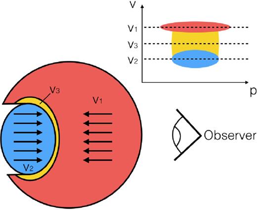
A schematic of a collision–observer system and a cartoon p–v diagram showing a broad bridge feature. Different colour components in the collision schematic correspond to the different colours on the p–v diagram.

Open in new tab Download slide

Figure 2.

An example CO (J = 1 → 0) p–v diagram of a possible cloud–cloud collision towards M20 (Torii et al. 2011). This p–v diagram is produced using data taken using Mopra and was presented in Haworth et al (2015).

Open in new tab Download slide

The intermediate-velocity gas is replenished as long as the collision is still occurring, so in order to remove the broad bridge feature the collision either needs to end (being fully braked or with one cloud punching right through the other) or the compressed dense layer resulting from the smaller cloud needs to be at least partially removed.

2.2 Details of the collision

We consider a collision between two clouds in a scenario similar to that discussed by Habe & Ohta (1992). One cloud of radius R₁ collides with a second, larger (R₂), cloud at velocity v_c. The entirety of the small cloud has been compressed after a time approximately given by t_c ≈ R₁/v_c (this is a lower limit, since it assumes that the post-collision velocity is small). We work in a frame in which the larger cloud is stationary. After t_c the compressed layer is still moving with some finite bulk velocity relative to the larger (in our frame, static) cloud, meaning that the broad bridge is still observable for some subsequent time-scale (to be determined below). Our considerations here are only very approximate, we do not include the effects of turbulence or instabilities that can arise in a compressive flow (e.g. McLeod & Whitworth 2013).

2.3 The collision time-scales

The broad bridge will disappear if the clouds break to the extent that they are no longer separated in velocity by more than half the sum of their turbulent velocity dispersions. If this happens, then only a single feature will appear in the p–v diagram. The broad bridge may also disappear if the smaller cloud punches right through the larger. To estimate these time-scales, we require a description of the smaller cloud velocity as a function of time.

2.3.1 Momentum-driven motion in the limit of constant deceleration

The smaller cloud (compressed layer) collides with the larger cloud in a frame in which the large cloud is initially static. We assume that all material from the larger cloud encountered by the compressed layer is swept up to travel with it. By conservation of momentum, this sweeping up of material decreases the velocity in the compressed layer and will lead to the collision being completely stalled after a distance

\begin{equation} D_{{\rm stag}} = \frac{2\rho _1R_1v_{\rm c}}{\rho _2v(t)}. \end{equation}

(1)

Assuming constant deceleration from the collision velocity v_c to zero

\begin{equation} \frac{\mathrm{d}v}{\mathrm{d}R} = \frac{v_{{\rm c}}}{D_{{\rm stag}}} = \frac{\rho _2v(t)}{2\rho _1R_1} \end{equation}

(2)

which yields

\begin{equation} \frac{\mathrm{d}v}{\mathrm{d}t}=\frac{\mathrm{d}v}{\mathrm{d}R}\frac{\mathrm{d}R}{\mathrm{d}t} = \frac{\rho _2v(t)^2}{2\rho _1R_1} \end{equation}

(3)

integrating this gives us a crude estimate of the velocity of the smaller cloud relative to the larger as a function of time

\begin{equation} v(t) = \frac{1}{\frac{\rho _2t}{2\rho _1R_1} + \frac{1}{v_{\rm c}}} = \frac{2R_1\rho _1v_{\rm c}}{\rho _2 tv_{\rm c} + 2\rho _1R_1}. \end{equation}

(4)

This is shown for the 20 km s⁻¹ collision between large clouds from Shima, Tasker & Habe (in preparation)as well as the 10 km s⁻¹ collision model from Takahira et al. (2014) in Fig. 3. The Shima et al. (in preparation) models include sink formation and radiative feedback, whereas the Takahira et al. (2014) models do not. Included in Fig. 3 are also points inferred from synthetic molecular line data cubes of the simulations (these synthetic observations will be discussed in more detail below). There are three time regions denoted on each plot. The leftmost region (t < t_c) is prior to the crossing time-scale of the smaller cloud. In this region, we do not necessarily expect good agreement because only some small fraction of the smaller cloud is undergoing collision, which the analytic model does not account for. In the middle time region, the whole small cloud is compressed into a layer travelling with a similar bulk velocity (ignoring turbulence), we therefore expect quite good agreement with our simple analytic estimate in this regime. The right-hand time region is beyond the time-scale that we predict the smaller cloud has exited the larger. In this region, it is again difficult to estimate the velocities from p–v maps since the broad bridge is completely removed or unclear. The derived estimates in this final time zone are made using a combination of p–v maps, the raw simulation data and line profiles.

Figure 3.

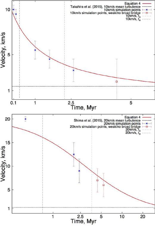
The velocity of the compressed layer as a function of time estimated using momentum balance and by assuming constant deceleration. The points are extracted from p–v diagrams/line profiles from synthetic data cubes of simulations (which we will discuss in Section 3). The width of the secondary peak in the broad bridge or ease with which two distinct velocity components can be identified determines the size of the error bars. The left-hand vertical line denotes the time after which the small cloud is compressed. The right-hand vertical line denotes the time after which the smaller cloud has punched through the larger.

Open in new tab Download slide

The simple analytic approximation reproduces the values seen in the simulations to within (at worst) ∼20 per cent and will therefore be a suitable tool for giving a first-order estimate of the time-scale over which the broad bridge survives due to the overall collision lifetime. Although after t_c the velocities predicted by our simple relation lie within the uncertainties (which are mostly based on how broad the two peaks of the broad bridge are), the simulations typically exhibit lower velocities than the analytic model predicts. This could be due to turbulent ram pressure braking the cloud further. The analytic solution also does not include gravity, which could affect the motion.

Equation (4) integrated until the collision velocity is less than half the sum of the two clouds turbulent velocity dispersions

\begin{equation} v(t)< \frac{1}{2}(\Delta v_1 + \Delta v_2), \end{equation}

(5)

or until the compressed layer escapes the larger cloud (traverses R₁ + R₂) gives us our first broad bridge lifetime estimate. For the latter criterion, we obtain an exit time-scale for the smaller cloud of

\begin{equation} t_e = \frac{2\rho _1R_1}{\rho _2v_{\rm c}}\left[\exp \left(\frac{\rho _2(R_1+R_2)}{2\rho _1R_1}\right)-1\right]. \end{equation}

(6)

This is our first broad bridge lifetime estimate, we will utilize it in Section 3.

2.4 Radiative feedback disruption time-scale

During the collision material is compressed into a dense layer, which continues to travel into the larger cloud, giving rise to the secondary feature in the p–v diagram. It is also within this dense region that star formation (possibly massive star formation) will occur. However, once stars have formed their ionizing radiation will result in bubbles of hot gas that might disrupt the dense layer, potentially rendering it unobservable (at least in molecular lines) once some fraction of it has been ionized.

For a star emitting N_ly ionizing photons per second into a medium of number density n a bubble of ionized gas results, with a ‘Strömgren’ radius (Strömgren 1939)

\begin{equation} r_{\rm s} = \left(\frac{3N_{{\rm ly}}}{4\pi n^2 \alpha _{{\rm B}}} \right)^{1/3}, \end{equation}

(7)

where α_B is the hydrogen case B recombination coefficient (that for recombinations in to all states other than the ground). This bubble is hot (10⁴ K) and overpressured relative to the ambient medium, meaning it expands. For our purposes, the extent of the H ii region (with sound speed c_i) under such so-called D-type expansion can be adequately described by the relation derived by Spitzer (1998)

\begin{equation} r(t) = r_{\rm s}\left(1 + \frac{7c_it}{4r_{\rm s}}\right)^{4/7} \end{equation}

(8)

(though the interested reader is directed towards Bisbas et al. 2015, for a discussion on the shortcomings and interpretation of the Spitzer solution, including how it differs from the solution derived by Hosokawa & Inutsuka 2006). As the ionized region expands, it will disrupt a larger volume of the material that makes up the broad bridge feature, until at some point it renders it undetectable.

We assume that the compressed layer has a length approximately the same as the smaller cloud diameter, 2 × R₁ and that the width is less than the Strömgren radius (see Appendix A). If this is the case, and we assume that the stars are centrally condensed in a cluster, then we only need to calculate the extent along the length of the layer that is ionized as a function of time. If the broad bridge is unobservable after some fraction f of the compressed layer is ionized, then we can calculate the broad bridge lifetime in the presence of radiative feedback using fR₁ = r(t), giving

\begin{equation} t_{\rm r} = \frac{4r_{\rm s}}{7c_i}\left[\left(\frac{fR_1}{r_{\rm s}}\right)^{7/4}-1\right]. \end{equation}

(9)

We can recast r_s in terms of collision variables. If the shock is isothermal, then the number density just behind the shock is

\begin{equation} n = \frac{\rho _2}{m_{\rm H}}\left(\frac{v_{\rm L}}{c_2}\right)^2 , \end{equation}

(10)

where v_L, ρ₂ and c₂ are the dense layer velocity and the larger cloud density and sound speed, respectively. Substituting equation (10) into equation (7) results in

\begin{equation} r_{\rm s} = \left(\frac{3N_{{\rm ly}} m_{\rm H}^2 c_2^4}{4\pi \alpha _{\rm B} \rho _2^2 v_{\rm L}^4}\right)^{1/3} \end{equation}

(11)

which combined with equation (9) gives us a radiative feedback disruption time-scale as a function of the large cloud density and collision velocity

\begin{equation} t_{\rm r} = \frac{4}{7c_i}\left(\frac{3N_{{\rm ly}} m_{\rm H}^2 c_2^4}{4\pi \alpha _{\rm B} \rho _2^2 v_{\rm L}^4}\right)^{1/3}\left[\left(\frac{fR_1}{\left(\frac{3N_{{\rm ly}} m_{\rm H}^2 c_2^4}{4\pi \alpha _{\rm B} \rho _2^2 v_{\rm L}^4}\right)^{1/3}}\right)^{7/4}-1\right]. \end{equation}

(12)

At the first level of approximation, we might set the dense layer velocity equal to the collision velocity (v_L = v_c). Indeed, if these equations are applied to observations, we suggest just using the observed collision velocity. However, for our discussion here it is more accurate to use the mean velocity over the lifetime of the broad bridge feature. To estimate the mean velocity, we first calculate an initial estimate of t_r using the velocity at the onset of collision v_c. We then calculate the mean velocity over this initial t_r time-scale estimate using equation (4). Lastly, we iterate over t_r and v_L until the fractional change in mean velocity is less than 1 per cent. Typical mean velocities over the radiative time-scale are around 40–60 per cent of the initial collision velocity.

We plot the disruption time-scale as a function of ionizing flux for different cloud/collision parameters in Fig. 4, each assuming that the clouds have a density of 100 m_H cm⁻³. We assume that the ionized and neutral gases have temperatures (sound speeds) of 10⁴ and 10 K (11.5 and 0.19 km s⁻¹), respectively. We also assume that the critical fraction of the cloud length that needs to be ionized is f = 0.5. Different lines in Fig. 4 correspond to different smaller cloud radii and collision velocities in the upper and lower panels, respectively. Since the radiative disruption time-scale scales as |$R_1^{7/4}$| but only |$N_{{\rm ly}}^{-1/4}$|⁠, a reduction of the cloud size by a factor of 10 requires a reduction in the ionizing luminosity by a factor of 10⁷ to maintain the same disruption time-scale. We therefore expect broad bridges to be disrupted more readily by radiative feedback in collision between smaller clouds, even if the ionizing luminosity is substantially lower. We will compare these relations with simulations in Section 3.

The time-scale for a broad bridge to be disrupted by radiative feedback as a function of ionizing flux. The upper panel is for a 20 km s−1 collision for different cloud radii. The lower panel is for a 10 pc cloud and different collision velocities. These plots assume that both colliding clouds have a density of 100 mH cm−3.

Figure 4.

The time-scale for a broad bridge to be disrupted by radiative feedback as a function of ionizing flux. The upper panel is for a 20 km s⁻¹ collision for different cloud radii. The lower panel is for a 10 pc cloud and different collision velocities. These plots assume that both colliding clouds have a density of 100 m_H cm⁻³.

Open in new tab Download slide

2.5 Stellar wind feedback disruption time-scale

We can estimate the effect of stellar wind feedback using a similar approach to that for radiative feedback. That is we can compare the size of a wind-blown bubble with the size of the compressed layer. We base our treatment of the expanding wind-blown region on the expansion in a cold uniform medium presented by Ngoumou et al. (2015), which in turn is based on Steigman, Strittmatter & Williams (1975) and Lamers & Cassinelli (1999). In this model, the bubble radius is given by

\begin{equation} r_{\rm w}(t) = 0.83\dot{M_{\rm w}}^{1/4}v_{\rm w}^{1/4}\rho _{\rm s}^{-1/4}t^{1/2}, \end{equation}

(13)

where |$\dot{M_{\rm w}}$|⁠, v_w and ρ_s are the wind mass loss rate, velocity and slab density (all in cgs units), respectively. Comparing equation (13) with some critical fraction of the layer size fR₁, and assuming an isothermal shock, gives a time at which disruption of the broad bridge due to winds takes place of

\begin{equation} t_{\rm w} = \frac{f^2R_1^2 \rho _2^{1/2} v_{\rm L}}{0.6889 \dot{M_{\rm w}}^{1/2}v_{\rm w}^{1/2} c_2}. \end{equation}

(14)

Note that this assumes that the total wind luminosity goes in to disrupting the broad bridge.

Plots of the broad bridge disruption time-scale as a function of wind luminosity for a variety of cloud sizes and collision velocities are given in Fig. 5. Note that in these plots we assume a wind velocity of 2000 km s⁻¹ and a gas density of 100 m_H cm⁻³. We again calculate the mean dense layer velocity using the iterative procedure discussed in Section 2.4.

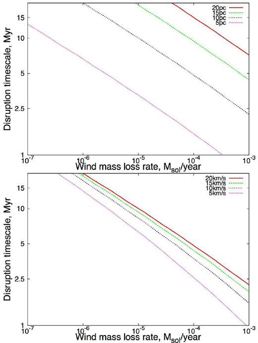
The time-scale for a broad bridge to be disrupted by stellar wind feedback as a function of wind luminosity for different cloud radii (at 20 km s−1 collision, top panel) and collision velocities (for a cloud of 10 pc radius, lower panel). The plots assume that both clouds have a density of 100 mH cm−3.

Figure 5.

The time-scale for a broad bridge to be disrupted by stellar wind feedback as a function of wind luminosity for different cloud radii (at 20 km s⁻¹ collision, top panel) and collision velocities (for a cloud of 10 pc radius, lower panel). The plots assume that both clouds have a density of 100 m_H cm⁻³.

Open in new tab Download slide

By comparing equation (12) with equation (14) for systems where (fR₁/r_s)^7/4 ≫ 1, our radiative feedback time-scale dominates over that for winds when

\begin{equation} \left(\frac{\dot{M_{\rm w}}}{10^{-6}\,{\rm M}_{\odot }\,\textrm {yr}^{-1}}\right) < 1.7 \left(\frac{R_1}{\textrm {pc}}\right)^{1/2}\left(\frac{N_{{\rm ly}}}{10^{48}\,\textrm {s}^{-1}}\right)^{1/2}, \end{equation}

(15)

where our assumed values are that the wind velocity is 2000 km s⁻¹, the ionized and neutral gas temperatures are 10⁴ and 10 K, respectively, f = 0.5 and case B recombination coefficient of 2.7 × 10⁻¹³ cm³ s⁻¹. According to previous numerical simulations by Dale et al. (2013, 2014) radiative feedback is typically expected to dominate over winds.

2.6 The star formation disruption time-scale

The gas mass depletion through star formation is roughly given by the time integral of the average star formation rate |$\dot{M}$|⁠. The broad bridge will be disrupted when some fraction F (which is probably different from the fraction of the length f discussed in the feedback time-scales) of the dense layer mass M_l is converted into stars

\begin{equation} \int \dot{M}{\rm d}t = FM_{{\rm l}}, \end{equation}

(16)

then the time-scale for star formation to remove the broad bridge is

\begin{equation} t_{{\rm sf}} = FM_{\rm l}/\dot{M}. \end{equation}

(17)

Unfortunately t₀, F, M_l and |$\dot{M}$| are all rather uncertain, so a more useful relation is difficult to derive. In subsequent comparison with numerical models in this paper, we therefore extract the values of t₀ and |$\dot{M}$| from the simulations. We assume that M_l is the smaller cloud mass and F is 0.5. This is the most uncertain time-scale in this paper.

2.7 Weaknesses of the analytic arguments

Our arguments made above are purely intended to provide rough lifetime estimates and to build an understanding of how feedback might disrupt the broad bridge feature. They may also assist in a basic interpretation of real observations. However, they have a number of shortcomings.

Simulations by Dale & Bonnell (2011) find that radiative feedback can be ineffective if the H ii region is substantially matter bounded. That is, if photons are able to stream freely from the ionized bubble. This would make radiative feedback much less effective than we predict and so will increase t_r.
Regarding both winds and ionizing radiation, we assume that the sources responsible for feedback are colocated. In reality, they will be distributed throughout the colliding layer.
At present there is no consideration of supernovae, which might also be effective at removing broad bridges after about 5 Myr.
We do not account for the effects of turbulence and assume constant deceleration in our collision time-scale estimate.
We assume that the collision is isothermal. In reality, the compressed layer density will likely larger than that given by the isothermal shock condition (equation 10), at least in the absence of turbulence.

3 NUMERICAL COMPARISON

We now study the evolution of the broad bridge feature in two numerical models and compare with our expectations from the analytic expressions. One of the models is without any form of feedback or sink formation, the second includes radiative feedback and sink formation. Neither include feedback from winds.

3.1 Numerical method

3.1.1 Hydrodynamic models

The hydrodynamic models that we post process are simulations of cloud–cloud collisions by Takahira et al. (2014) and Shima et al. (in preparation). These models were both run using the grid-based radiation hydrodynamics code enzo (Bryan et al. 2014). They both consider head-on collisions between two non-identical, turbulent clouds.

The collision with feedback and sink particles is the 20 km s⁻¹ collision model from Shima et al. (in preparation). A summary of the cloud parameters is given in Table 1. Once sink particles form in this simulation, they are assumed to have an ionizing luminosity of 3 × 10⁴⁶ photons s⁻¹ M|$_{{\odot }}^{-1}$|⁠. In this model, both clouds are travelling in opposite directions at 10 km s⁻¹. We consider snapshots at 0.4, 2, 2.4, 4.4 and 5.4 Myr after the onset of collision. At 2.4 Myr, there is approximately 100 M_ȯ in sink particles, implying an ionizing flux of 3 × 10⁴⁸ photons s⁻¹; this is the value we use in our radiative feedback disruption time-scale estimate.

Table 1.

Open in new tab

Summary of the parameters of the feedback model from Shima et al. (in preparation).

Parameter	Value	Description
R₁	14.45 pc	Smaller cloud radius
R₂	27.93 pc	Larger cloud radius
ρ₁	24.4 m_H cm⁻³	Smaller cloud density
ρ₂	11.79 m_H cm⁻³	Larger cloud density
v_c	20 km s⁻¹	Collision velocity
Δv₁	1 km s⁻¹	Smaller cloud turbulent velocity
Δv₂	1.49 km s⁻¹	Larger cloud turbulent velocity
Q	3 × 10⁴⁶ s⁻¹ M\|$_{{\odot }}^{-1}$\|	Ionizing flux per solar mass
Q_tot	3 × 10⁴⁸ s⁻¹	Total ionizing flux after 2.4 Myr
		of collision

Parameter	Value	Description
R₁	14.45 pc	Smaller cloud radius
R₂	27.93 pc	Larger cloud radius
ρ₁	24.4 m_H cm⁻³	Smaller cloud density
ρ₂	11.79 m_H cm⁻³	Larger cloud density
v_c	20 km s⁻¹	Collision velocity
Δv₁	1 km s⁻¹	Smaller cloud turbulent velocity
Δv₂	1.49 km s⁻¹	Larger cloud turbulent velocity
Q	3 × 10⁴⁶ s⁻¹ M\|$_{{\odot }}^{-1}$\|	Ionizing flux per solar mass
Q_tot	3 × 10⁴⁸ s⁻¹	Total ionizing flux after 2.4 Myr
		of collision

Table 1.

Open in new tab

Summary of the parameters of the feedback model from Shima et al. (in preparation).

Parameter	Value	Description
R₁	14.45 pc	Smaller cloud radius
R₂	27.93 pc	Larger cloud radius
ρ₁	24.4 m_H cm⁻³	Smaller cloud density
ρ₂	11.79 m_H cm⁻³	Larger cloud density
v_c	20 km s⁻¹	Collision velocity
Δv₁	1 km s⁻¹	Smaller cloud turbulent velocity
Δv₂	1.49 km s⁻¹	Larger cloud turbulent velocity
Q	3 × 10⁴⁶ s⁻¹ M\|$_{{\odot }}^{-1}$\|	Ionizing flux per solar mass
Q_tot	3 × 10⁴⁸ s⁻¹	Total ionizing flux after 2.4 Myr
		of collision

Parameter	Value	Description
R₁	14.45 pc	Smaller cloud radius
R₂	27.93 pc	Larger cloud radius
ρ₁	24.4 m_H cm⁻³	Smaller cloud density
ρ₂	11.79 m_H cm⁻³	Larger cloud density
v_c	20 km s⁻¹	Collision velocity
Δv₁	1 km s⁻¹	Smaller cloud turbulent velocity
Δv₂	1.49 km s⁻¹	Larger cloud turbulent velocity
Q	3 × 10⁴⁶ s⁻¹ M\|$_{{\odot }}^{-1}$\|	Ionizing flux per solar mass
Q_tot	3 × 10⁴⁸ s⁻¹	Total ionizing flux after 2.4 Myr
		of collision

The collision without feedback or sink particles (i.e. without star formation) is the 10 km s⁻¹ collision model from Takahira et al. (2014). A summary of the clouds parameters is given in Table 2. In this model, the collision is in such a frame that the larger cloud is stationary. We consider snapshots at 0.1, 0.2, 1, 1.6, 2.6 and 4.4 Myr after the onset of the collision.

Table 2.

Open in new tab

Summary of the parameters of the feedback model from Takahira et al (2014).

Parameter	Value	Description
R₁	3.5 pc	Smaller cloud radius
R₂	7.2 pc	Larger cloud radius
ρ₁	47.4 m_H cm⁻³	Smaller cloud density
ρ₂	25.3 m_H cm⁻³	Larger cloud density
v_c	10 km s⁻¹	Collision velocity
Δv₁	1.25 km s⁻¹	Smaller cloud turbulent velocity
Δv₂	1.71 km s⁻¹	Larger cloud turbulent velocity

Parameter	Value	Description
R₁	3.5 pc	Smaller cloud radius
R₂	7.2 pc	Larger cloud radius
ρ₁	47.4 m_H cm⁻³	Smaller cloud density
ρ₂	25.3 m_H cm⁻³	Larger cloud density
v_c	10 km s⁻¹	Collision velocity
Δv₁	1.25 km s⁻¹	Smaller cloud turbulent velocity
Δv₂	1.71 km s⁻¹	Larger cloud turbulent velocity

Table 2.

Open in new tab

Summary of the parameters of the feedback model from Takahira et al (2014).

Parameter	Value	Description
R₁	3.5 pc	Smaller cloud radius
R₂	7.2 pc	Larger cloud radius
ρ₁	47.4 m_H cm⁻³	Smaller cloud density
ρ₂	25.3 m_H cm⁻³	Larger cloud density
v_c	10 km s⁻¹	Collision velocity
Δv₁	1.25 km s⁻¹	Smaller cloud turbulent velocity
Δv₂	1.71 km s⁻¹	Larger cloud turbulent velocity

Parameter	Value	Description
R₁	3.5 pc	Smaller cloud radius
R₂	7.2 pc	Larger cloud radius
ρ₁	47.4 m_H cm⁻³	Smaller cloud density
ρ₂	25.3 m_H cm⁻³	Larger cloud density
v_c	10 km s⁻¹	Collision velocity
Δv₁	1.25 km s⁻¹	Smaller cloud turbulent velocity
Δv₂	1.71 km s⁻¹	Larger cloud turbulent velocity

3.1.2 Radiative transfer

As for our original synthetic observations in Haworth et al. (2015), we use the torus radiation transport and hydrodynamics code to post-process simulations in this paper (Harries 2000; Kurosawa et al. 2004; Haworth & Harries 2012). In particular, we use the molecular line transfer algorithm discussed by Rundle et al. (2010) and Haworth et al. (2013). torus is capable of non-local thermodynamic equilibrium (LTE) statistical equilibrium calculations, which were used in Haworth et al. (2015); however, since we are post-processing a relatively large number of snapshots in order to study the time evolution of broad bridges we assume LTE when calculating the molecular level populations in this paper. This does not alter the qualitative p–v diagram (we are only studying the morphological evolution) and substantially reduces our computational expense. With the level populations calculated, a synthetic data cube is generated using ray tracing (Rundle et al. 2010). This data cube is manipulated using the starlink image analysis tool gaia to produce p–v maps. In this paper, we produce synthetic ¹²CO (J = 1 → 0) data assuming an abundance relative to hydrogen of 8 × 10⁻⁵.

3.2 Results of synthetic observations

3.2.1 20 km s⁻¹ collision model from Shima et al. (in preparation)

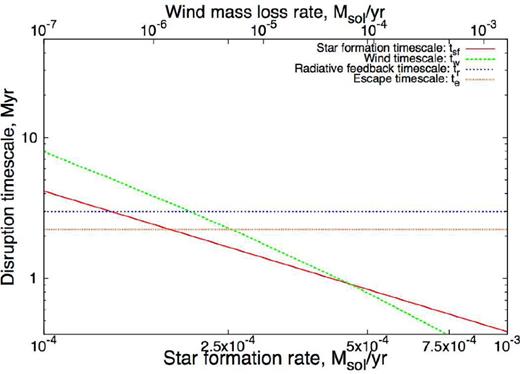
We first apply our analytic arguments to a 20 km s⁻¹ collision between two large clouds studied by Shima et al. (in preparation). The parameters of this model are given in Table 1. In Fig. 6, we plot the broad bridge disruption time-scales based on the exit time-scale (equation 6), wind/radiative feedback (equations 9 and 14) and star formation rate (equation 17) for this model. We allow the star formation rate and wind mass-loss rate to vary and use the known ionizing flux of stars in the simulation at 2.4 Myr (3 ×10⁴⁸ photons s⁻¹). From these disruption time-scales, we expect the broad bridge to be first disrupted after about 3.5 Myr because the smaller cloud has exited the larger (see the red small-dotted horizontal line in Fig. 6). High star formation rates or wind mass-loss rates are required to disrupt the broad bridge on a comparable time-scale. We expect that radiative feedback would require about 11 Myr to clear the broad bridge.

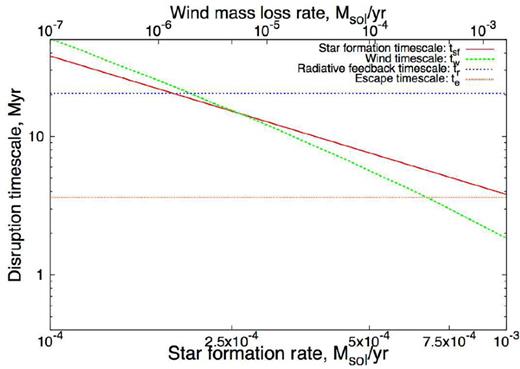
Various time-scales for associated with the broad bridge for the 20 km s−1 collision model from Shima et al. (in preparation). tsf, tr and tw are the time it takes for star formation, radiative feedback and wind feedback to quench the broad bridge. te is the time it takes for the small cloud to punch through the larger cloud.

Figure 6.

Various time-scales for associated with the broad bridge for the 20 km s⁻¹ collision model from Shima et al. (in preparation). t_sf, t_r and t_w are the time it takes for star formation, radiative feedback and wind feedback to quench the broad bridge. t_e is the time it takes for the small cloud to punch through the larger cloud.

Open in new tab Download slide

Fig. 7 shows the p–v diagram for this model at 0.4, 2, 2.4 and 4.4 Myr after the onset of collision. In the upper-left panel, the clouds have only just begun colliding. This snapshot is at a time earlier than the time-scale for crossing the small cloud at the collision velocity. At this stage in the collision, the p–v diagram just looks like clouds coincident along the line of sight (though there is some very weak intermediate-velocity emission). As the collision progresses the broad bridge forms, getting harder to identify as the two intensity peaks approach one another and as the smaller cloud's signature becomes more disordered. By 4.4 Myr (bottom-right panel), the broad bridge is obviously not present, consistent with the result expected from our simple analytic estimates. Although the broad bridge is not observable, there is disordered emission from gas over a 10 km s⁻¹ velocity range at this time. By 4.4 Myr, the larger cloud's feature has also started to be significantly disrupted. The larger feature also appears to decrease in velocity dispersion with time (its thickness along the velocity axis decreases). This is due to dissipation of the turbulence, either by collisions or dilution in the wider interstellar medium.

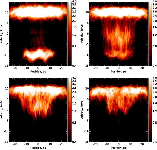
12CO (J = 1 → 0) synthetic p–v diagrams of snapshots from the 20 km s−1 collision model from Shima et al. (in preparation). The panels are for snapshots at 0.4 (top left), 2 (top right), 2.4 (bottom left) and 4.4 Myr (bottom right).

Figure 7.

¹²CO (J = 1 → 0) synthetic p–v diagrams of snapshots from the 20 km s⁻¹ collision model from Shima et al. (in preparation). The panels are for snapshots at 0.4 (top left), 2 (top right), 2.4 (bottom left) and 4.4 Myr (bottom right).

Open in new tab Download slide

Our analytic arguments give a broad bridge lifetime consistent with the observations to within at least 1 Myr in this case. According to these arguments, the broad bridge lifetime in this scenario is determined by the collision lifetime, rather than feedback. Though it is likely that conversion of gas into stars, feedback and the collision lifetime do all cumulatively contribute, meaning that the collision lifetime estimate is likely an upper limit on the broad bridge lifetime.

3.2.2 10 km s⁻¹ collision model from Takahira et al (2014)

We now apply our analytic arguments to the 10 km s⁻¹ collision model from Takahira et al. (2014), the parameters of which are summarized in Table 2. Unlike in the previous model, this does not include any radiative feedback or star formation. The disruption time-scales for this model are shown in Fig. 8, where we assume an ionizing luminosity an order of magnitude lower than that in the previous model (10⁴⁷ photons s⁻¹). In this collision between smaller clouds, our analytic arguments predict that star formation as well as radiative and wind feedback will be much more effective at disrupting the broad bridge – to the extent that they can readily dominate over the collision time-scale. Recall that since the radiative disruption time-scale scales as |$R_{\rm s}^{7/4}$| but only |$N_{{\rm ly}}^{-1/4}$|⁠, a reduction of the cloud size by a factor of 10 requires a reduction in the ionizing luminosity by a factor of 10⁷ to maintain the same disruption time-scale. The simulations in Takahira et al. (2014) did not include star formation or feedback. Since the predicted escape time-scale is smaller than the radiative one, we do not expect radiative feedback to be important to the broad bridge lifetime.

Various time-scales for associated with the broad bridge for the 10 km s−1 collision model from Takahira et al (2014). tsf, tr and tw are the time it takes for star formation, radiative feedback and wind feedback to quench the broad bridge. te is the time it takes for the small cloud to punch through the larger cloud.

Figure 8.

Various time-scales for associated with the broad bridge for the 10 km s⁻¹ collision model from Takahira et al (2014). t_sf, t_r and t_w are the time it takes for star formation, radiative feedback and wind feedback to quench the broad bridge. t_e is the time it takes for the small cloud to punch through the larger cloud.

Open in new tab Download slide

p–v diagrams for snapshots of this model at 0.1, 1, 1.6 and 2.6 Myr are shown in Fig. 9. There is similar evolution to the other collisional model, only with less small-scale clumpy structure due to the lack of conversion of gas into stars, as well as a lack of feedback. The bottom-right panel of Fig. 9 is 0.2 Myr after the exit time-scale predicts that the broad bridge should be disrupted. Although some remnant of a secondary intensity peak remains, it has been predominantly disrupted and is no longer so ‘broad’. The actual exit time in the simulation is about 2.8 Myr, compared to our analytic estimate of 2.2 Myr. This difference is consistent with our findings in Section 2.3.1, where the actual collision velocity in the simulations was typically slightly lower than the analytic relations predict. This is due to lack of treatment of processes such as turbulent pressure and gravity.

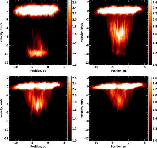
12CO (J = 1 → 0) synthetic p–v diagrams of snapshots from the 10 km s−1 collision model from Takahira et al. (2014). The panels are for snapshots at 0.1 (top left), 1 (top right), 1.6 (bottom left) and 2.6 Myr (bottom right).

Figure 9.

¹²CO (J = 1 → 0) synthetic p–v diagrams of snapshots from the 10 km s⁻¹ collision model from Takahira et al. (2014). The panels are for snapshots at 0.1 (top left), 1 (top right), 1.6 (bottom left) and 2.6 Myr (bottom right).

Open in new tab Download slide

4 DISCUSSION

4.1 On the cloud–cloud collision rate

We have developed tools for estimating broad bridge lifetimes which, where testable, seem to be consistent with our numerical models. In general, we expect broad bridge lifetimes of around 1–5 Myr. To date, seven broad bridge features have been identified in the Galaxy. Six of these are strong: M20 (Torii et al. 2011; Haworth et al. 2015), RCW 120 (Torii et al. 2015), NGC 3603 (Fukui et al. 2014), RCW 38 (Fukui et al. 2015), NGC 6334 and NGC 6357. Westerlund 2 also shows a weak broad bridge feature (Furukawa et al. 2009). Dobbs et al. (2015) predict collisions of the order 1 every 10 Myr for clouds of size 10 pc or larger, which would be inconsistent with the amount of broad bridge features currently observed (which are a lower limit, given that more may yet be observed) if our typical broad bridge lifetimes are correct.

However, in order for the number of broad bridges to not be extremely large (or zero), there should always be approximately an equilibrium number of broad bridges. In order to achieve a steady state, the rate at which broad bridges are formed must be approximately equal to the destruction rate. We can hence use our analytic arguments to estimate the equilibrium collision rate as a function of cloud size. We do this in Fig. 10 for 10 km s⁻¹ collisions. We assume that the larger cloud radius is twice that of the smaller. We assume that the smaller cloud has a density that scales as

\begin{equation} n = \max \left(-2.1*\frac{R}{\textrm {pc}} + 54.75, 10\right) \end{equation}

(18)

(which is based on the radii and densities of the clouds in the dynamical models discussed here) and that the larger cloud is half of this density. We also assume that the ionizing luminosity of the resulting stars varies with colliding cloud sizes as

\begin{equation} N_{{\rm ly}} = \left(\frac{3\times 10^{48}R_1}{14.45\,\textrm {pc}}\right)^{-2}\,\textrm {s}^{-1} \end{equation}

(19)

which is motivated by the Shima et al. (in preparation) simulation. We only consider the maximum required collision rate based on the exit time-scale (equation 6) and the radiative feedback time-scale (equation 12).

Figure 10.

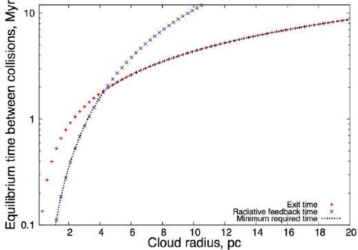
The time between cloud–cloud collisions as a function of cloud radius assuming that an equilibrium number of broad bridge features is maintained. This is for collision parameters discussed in Section 4.1.

Open in new tab Download slide

For clouds larger than about 5 pc, the exit time-scales require collision rates consistent with those calculated by Dobbs et al. (2015), but for smaller clouds (not identified in the Dobbs et al. 2015, estimates) the collision rates are expected to be much higher (this is required by both the exit and radiative feedback time-scales). Of the systems observed to host broad bridges, NGC 6334 and NGC 6357 are approximately 10 pc in size; however, all others are less than 4 pc. For the example of M20 which is about 2 pc in size, from our equilibrium consideration we expect about four such collisions per Myr. This is in contrast to the Dobbs et al. (2015) general value of about 1 per 10 Myr. It is therefore possible that high cloud–cloud collision rates, leading to massive star formation, are present in the Galaxy that are not contradictory to those rates expected from Dobbs et al. (2015). Higher collision rates for smaller clouds could be tested using new galactic models that are able to identify clouds below 10 pc in size. If higher collision rates for smaller clouds are found, this would call for further detailed simulations of the collisional process. In particular, to understand the link between the properties of the colliding clouds (e.g. radius, density, turbulence, collision velocity) and any subsequent star formation (e.g. star formation efficiency and mass spectrum), which might be compared with observations of candidate collision sites.

5 SUMMARY AND CONCLUSIONS

We study the lifetimes of broad bridge features in p–v diagrams. We do so using a combination of analytic arguments and by post-processing hydrodynamic and radiation hydrodynamic simulations of cloud–cloud collisions. We draw the following main conclusions from this work.

We derived simple analytical tools to estimate broad bridge lifetimes. The lifetime of the broad bridge is constrained by either the collision time-scale, the time-scales for disruption by winds or radiative feedback and the time-scale for the depletion of gas through star formation.
The radiative feedback lifetime t_R scales with the ionizing flux as |$t_{\rm R}\propto N_{{\rm ly}}^{-1/4}$| and the smaller cloud radius as |$t_{\rm R}\propto R_{\rm s}^{7/4}$|⁠. This implies that to maintain a given radiative feedback disruption time-scale for smaller clouds, the ionizing flux needs to be more drastically reduced. Due to this effect, although larger clouds have their broad bridge lifetimes determined by the collision time-scale, for smaller clouds feedback can play a dominant role in determining the broad bridge lifetime.
If we assume that there should be some constant number of broad bridges with time, then the disruption time-scales should be roughly equal to the time between collisions at a given cloud size. If this is the case, our disruption time-scales give collision rate estimates. We find that such estimates are readily consistent with the 1 per 10 Myr collision rate estimates by Dobbs et al. (2015) for clouds larger than about 6 pc. However, for smaller clouds (which Dobbs et al. 2015, do not consider) we find much high collision rates, for example 4 per Myr for 2 pc radius clouds.
Given conclusion (3) and the fact that most high-mass star formation sites where broad bridges have been identified are less than 4 pc in size, we suggest that a large number of smaller scale cloud–cloud collisions could be triggering a substantial amount of high-mass star formation.

ACKNOWLEDGMENTS

We thank the referee for their insightful and thorough review, which led to the introduction of some interesting new aspects to the paper. TJH is funded by the STFC consolidated grant ST/K000985/1. EJT is funded by the MEXT grant for the Tenure Track System. Enzo simulations were carried out on the Cray XC30 at the Center for Computational Astrophysics (CfCA) of the National Astronomical Observatory of Japan. This research was supported by the DFG cluster of excellence ‘Origin and Structure of the Universe (JED)’. AH is supported by JSPS KAKENHI Grant Number 15K05014.

REFERENCES

Anathpindika

S. V.

2010

,

MNRAS

,

405

,

1431

Bisbas

T. G.

et al.

2015

,

MNRAS

,

453

,

1324

Crossref

Search ADS

Bryan

G. L.

et al.

2014

,

ApJS

,

211

,

19

Crossref

Search ADS

Clarke

C.

,

Carswell

B.

2007

,

Principles of Astrophysical Fluid Dynamics

.

Cambridge Univ. Press

,

Cambridge

Google Scholar

Google Preview

OpenURL Placeholder Text

WorldCat

Dale

J. E.

,

Bonnell

I.

2011

,

MNRAS

,

414

,

321

Crossref

Search ADS

Dale

J. E.

,

Ngoumou

J.

,

Ercolano

B.

,

Bonnell

I. A.

2013

,

MNRAS

,

436

,

3430

Crossref

Search ADS

Dale

J. E.

,

Ngoumou

J.

,

Ercolano

B.

,

Bonnell

I. A.

2014

,

MNRAS

,

442

,

694

Crossref

Search ADS

Dobbs

C. L.

,

Pringle

J. E.

,

Duarte-Cabral

A.

2015

,

MNRAS

,

446

,

3608

Crossref

Search ADS

Fukui

Y.

et al.

2014

,

ApJ

,

780

,

36

Crossref

Search ADS

Fukui

Y.

et al.

2015

,

preprint (arXiv:1504.05391)

Furukawa

N.

,

Dawson

J. R.

,

Ohama

A.

,

Kawamura

A.

,

Mizuno

N.

,

Onishi

T.

,

Fukui

Y.

2009

,

ApJ

,

696

,

L115

Crossref

Search ADS

Habe

A.

,

Ohta

K.

1992

,

PASJ

,

44

,

203

Harries

T. J.

2000

,

MNRAS

,

315

,

722

Crossref

Search ADS

Haworth

T. J.

,

Harries

T. J.

2012

,

MNRAS

,

420

,

562

Crossref

Search ADS

Haworth

T. J.

,

Harries

T. J.

,

Acreman

D. M.

,

Rundle

D. A.

2013

,

MNRAS

,

431

,

3470

Crossref

Search ADS

Haworth

T. J.

et al.

2015

,

MNRAS

,

450

,

10

Crossref

Search ADS

Hosokawa

T.

,

Inutsuka

S.-i.

2006

,

ApJ

,

646

,

240

Crossref

Search ADS

Inoue

T.

,

Fukui

Y.

2013

,

ApJ

,

774

,

L31

Crossref

Search ADS

Kurosawa

R.

,

Harries

T. J.

,

Bate

M. R.

,

Symington

N. H.

2004

,

MNRAS

,

351

,

1134

Crossref

Search ADS

Lamers

H. J. G. L. M.

,

Cassinelli

J. P.

1999

,

Introduction to Stellar Winds

.

Cambridge Univ. Press

,

Cambridge

Google Scholar

Google Preview

OpenURL Placeholder Text

WorldCat

McLeod

A. D.

,

Whitworth

A. P.

2013

,

MNRAS

,

431

,

710

Crossref

Search ADS

Ngoumou

J.

,

Hubber

D.

,

Dale

J. E.

,

Burkert

A.

2015

,

ApJ

,

798

,

32

Crossref

Search ADS

Ricotti

M.

,

Ferrara

A.

,

Miniati

F.

1997

,

ApJ

,

485

,

254

Crossref

Search ADS

Rundle

D.

,

Harries

T. J.

,

Acreman

D. M.

,

Bate

M. R.

2010

,

MNRAS

,

407

,

986

Crossref

Search ADS

Spitzer

L.

1998

,

Physical Processes in the Interstellar Medium

.

Wiley

,

New York

Google Scholar

Google Preview

OpenURL Placeholder Text

WorldCat

Steigman

G.

,

Strittmatter

P. A.

,

Williams

R. E.

1975

,

ApJ

,

198

,

575

Crossref

Search ADS

Stone

M. E.

1970

,

ApJ

,

159

,

277

Crossref

Search ADS

Strömgren

B.

1939

,

ApJ

,

89

,

526

Crossref

Search ADS

Takahira

K.

,

Tasker

E. J.

,

Habe

A.

2014

,

ApJ

,

792

,

63

Crossref

Search ADS

Tasker

E. J.

2011

,

ApJ

,

730

,

11

Crossref

Search ADS

Tasker

E. J.

,

Tan

J. C.

2009

,

ApJ

,

700

,

358

Crossref

Search ADS

Tasker

E. J.

,

Wadsley

J.

,

Pudritz

R.

2015

,

ApJ

,

801

,

33

Crossref

Search ADS

Torii

K.

et al.

2011

,

ApJ

,

738

,

46

Crossref

Search ADS

Torii

K.

et al.

2015

,

ApJ

,

806

,

7

Crossref

Search ADS

Umekawa

M.

,

Matsumoto

R.

,

Miyaji

S.

,

Yoshida

T.

1999

,

PASJ

,

51

,

625

Whitworth

A. P.

,

Bhattal

A. S.

,

Chapman

S. J.

,

Disney

M. J.

,

Turner

J. A.

1994

,

MNRAS

,

268

,

291

Crossref

Search ADS

Wu

B.

,

Van Loo

S.

,

Tan

J. C.

,

Bruderer

S.

2015

,

preprint (arXiv:1503.01873)

APPENDIX A: THE THICKNESS OF THE DENSE LAYER

Here we discuss the assumption that the slab thickness is less than the Strömgren radius. We begin by noting that this criterion is not essential and that so long as the layer is not much larger than the Strömgren radius (meaning that the H ii region will expand beyond the slab thickness quite quickly) our results are unaffected.

We can approximate the dense layer as a self-gravitating isothermal slab, for which the density distribution is given by

\begin{equation} \rho _{\rm L}(z) = \rho _{\rm L}(0)\,\textrm {sech}^2\left(\frac{z}{H}\right), \end{equation}

(A1)

where the scaleheight is

\begin{equation} H = \left(\frac{c_{\rm s}^2}{2 \pi G \rho _{\rm L}}\right)^{1/2} = \left(\frac{c_{\rm s}^4}{2 \pi G \rho _2 v_{\rm L}^2}\right)^{1/2} \end{equation}

(A2)

(see e.g. Umekawa et al. 1999; Clarke & Carswell 2007). We assume that the slab sound speed c_s is the same as for all neutral gas (i.e. the same as that in the neutral colliding clouds). Equating this scaleheight to the Strömgren radius (equation 11), we find that the assumption that the Strömgren radius is larger than the slab width applies wherever

\begin{equation} N_{{\rm ly}} > \frac{ 2^{1/2}\alpha _{\rm B} c_{\rm s}^2v_{\rm L} n_2^{1/2}}{3\pi ^{1/2}(Gm_{\rm H})^{3/2}}, \end{equation}

(A3)

which, inserting standard values, can be expressed as

\begin{equation} \left(\frac{N_{{\rm ly}}}{10^{46}}\right) > 6.85 \left(\frac{v_{\rm L}}{\textrm {km s}^{-1}}\right)\left(\frac{n_2}{\textrm {cm}^{-3}}\right)^{1/2}, \end{equation}

(A4)

where we remind the reader that v_L is the dense layer velocity and n₂ is the density in the larger cloud. For the example of the Shima et al. (in preparation) collision (discussed here in Section 3.2.1) we find a predicted slab scaleheight of 0.05 pc (so a slab width of about 0.1 pc) and that equation (A4) is satisfied. We remind the reader that this analysis assumes that the ionizing sources are centrally located.

A similar consideration can be made for winds by comparing equations (A2) and (13), which tells us that the wind will break out of the slab after a time

\begin{eqnarray} \left(\frac{t}{\textrm {yr}}\right) > 50.67 \left(\frac{v_{\rm L}}{\textrm {km s}^{-1}}\right)^{-1} \left(\frac{v_{\rm w}}{\textrm {2000 km s}^{-1}}\right)^{-1/2} \nonumber\\ \times \left(\frac{n_2}{\textrm {cm}^{-3}}\right)^{-1/2} \left(\frac{\dot{M}}{\textrm {M}_{{\odot }}\,\textrm {yr}^{-1}}\right)^{-1/2}. \end{eqnarray}

(A5)

We note that if ram pressure dominates over self-gravity, then the dense layer description of Whitworth et al. (1994) would be more appropriate than the self-gravitating one considered here.

Download all slides

Month:	Total Views:
January 2017	5
February 2017	7
March 2017	5
April 2017	6
May 2017	6
June 2017	5
July 2017	19
August 2017	7
September 2017	10
October 2017	3
November 2017	3
December 2017	5
January 2018	2
February 2018	2
March 2018	8
April 2018	5
May 2018	4
June 2018	8
July 2018	4
August 2018	5
October 2018	2
November 2018	2
December 2018	3
January 2019	7
February 2019	10
March 2019	10
April 2019	9
May 2019	7
June 2019	16
July 2019	12
August 2019	12
September 2019	15
October 2019	32
November 2019	17
December 2019	21
January 2020	19
February 2020	18
March 2020	10
April 2020	9
May 2020	5
June 2020	14
July 2020	7
August 2020	7
September 2020	12
October 2020	7
November 2020	9
December 2020	6
January 2021	5
February 2021	7
March 2021	10
April 2021	5
May 2021	5
June 2021	4
July 2021	7
August 2021	2
September 2021	5
October 2021	8
November 2021	6
December 2021	2
January 2022	13
February 2022	9
March 2022	13
April 2022	11
May 2022	6
June 2022	11
July 2022	36
August 2022	12
September 2022	10
October 2022	5
November 2022	7
December 2022	3
January 2023	3
February 2023	3
March 2023	5
April 2023	8
May 2023	3
June 2023	5
July 2023	2
August 2023	9
September 2023	2
October 2023	8
November 2023	4
December 2023	9
January 2024	13
February 2024	12
March 2024	17
April 2024	15
May 2024	15
June 2024	13
July 2024	23
August 2024	20
September 2024	23
October 2024	21
November 2024	14
December 2024	8
January 2025	8
February 2025	13
March 2025	21
April 2025	11
May 2025	6

Article Contents

Isolating signatures of major cloud–cloud collisions – II. The lifetimes of broad bridge features

ABSTRACT

1 INTRODUCTION

2 ANALYTIC ARGUMENTS REGARDING THE TIME-SCALE FOR DISRUPTION OF BROAD BRIDGES

2.1 Preamble: what is the broad bridge

2.2 Details of the collision

2.3 The collision time-scales

2.3.1 Momentum-driven motion in the limit of constant deceleration

2.4 Radiative feedback disruption time-scale

2.5 Stellar wind feedback disruption time-scale

2.6 The star formation disruption time-scale

2.7 Weaknesses of the analytic arguments

3 NUMERICAL COMPARISON

3.1 Numerical method

3.1.1 Hydrodynamic models

3.1.2 Radiative transfer

3.2 Results of synthetic observations

3.2.1 20 km s⁻¹ collision model from Shima et al. (in preparation)

3.2.2 10 km s⁻¹ collision model from Takahira et al (2014)

4 DISCUSSION

4.1 On the cloud–cloud collision rate

5 SUMMARY AND CONCLUSIONS

ACKNOWLEDGMENTS

REFERENCES

APPENDIX A: THE THICKNESS OF THE DENSE LAYER

Citations

Views

Altmetric

Email alerts

Astrophysics Data System

Citing articles via

Latest

Most Read

Most Cited

Article Contents

Isolating signatures of major cloud–cloud collisions – II. The lifetimes of broad bridge features Free

ABSTRACT

1 INTRODUCTION

2 ANALYTIC ARGUMENTS REGARDING THE TIME-SCALE FOR DISRUPTION OF BROAD BRIDGES

2.1 Preamble: what is the broad bridge

2.2 Details of the collision

2.3 The collision time-scales

2.3.1 Momentum-driven motion in the limit of constant deceleration

2.4 Radiative feedback disruption time-scale

2.5 Stellar wind feedback disruption time-scale

2.6 The star formation disruption time-scale

2.7 Weaknesses of the analytic arguments

3 NUMERICAL COMPARISON

3.1 Numerical method

3.1.1 Hydrodynamic models

3.1.2 Radiative transfer

3.2 Results of synthetic observations

3.2.1 20 km s−1 collision model from Shima et al. (in preparation)

3.2.2 10 km s−1 collision model from Takahira et al (2014)

4 DISCUSSION

4.1 On the cloud–cloud collision rate

5 SUMMARY AND CONCLUSIONS

ACKNOWLEDGMENTS

REFERENCES

APPENDIX A: THE THICKNESS OF THE DENSE LAYER

Citations

Views

Altmetric

Email alerts

Astrophysics Data System

Citing articles via

Latest

Most Read

Most Cited

This Feature Is Available To Subscribers Only

Isolating signatures of major cloud–cloud collisions – II. The lifetimes of broad bridge features

3.2.1 20 km s⁻¹ collision model from Shima et al. (in preparation)

3.2.2 10 km s⁻¹ collision model from Takahira et al (2014)