Simulating the 21 cm forest detectable with LOFAR and SKA in the spectra of high-z GRBs

Ciardi, B.; Inoue, S.; Abdalla, F. B.; Asad, K.; Bernardi, G.; Bolton, J. S.; Brentjens, M.; de Bruyn, A. G.; Chapman, E.; Daiboo, S.; Fernandez, E. R.; Ghosh, A.; Graziani, L.; Harker, G. J. A.; Iliev, I. T.; Jelić, V.; Jensen, H.; Kazemi, S.; Koopmans, L. V. E.; Martinez, O.; Maselli, A.; Mellema, G.; Offringa, A. R.; Pandey, V. N.; Schaye, J.; Thomas, R.; Vedantham, H.; Yatawatta, S.; Zaroubi, S.

doi:10.1093/mnras/stv1640

Abstract

We investigate the feasibility of detecting 21 cm absorption features in the afterglow spectra of high redshift long Gamma Ray Bursts (GRBs). This is done employing simulations of cosmic reionization, together with estimates of the GRB radio afterglow flux and the instrumental characteristics of the LOw Frequency ARray (LOFAR). We find that absorption features could be marginally (with a S/N larger than a few) detected by LOFAR at z ≳ 7 if the GRB is a highly energetic event originating from Pop III stars, while the detection would be easier if the noise were reduced by one order of magnitude, i.e. similar to what is expected for the first phase of the Square Kilometre Array (SKA1-low). On the other hand, more standard GRBs are too dim to be detected even with ten times the sensitivity of SKA1-low, and only in the most optimistic case can a S/N larger than a few be reached at z ≳ 9.

gamma-ray burst: general, dark ages, reionization, first stars, radio lines: general

1 INTRODUCTION

Present and planned radio facilities such as LOFAR¹ (van Haarlem et al. 2013), MWA,² PAPER³ and SKA,⁴ aim at detecting the 21 cm signal from the Epoch of Reionization (EoR) in terms of observations such as tomography (e.g. Tozzi et al. 2000; Ciardi & Madau 2003; Furlanetto, Sokasian & Hernquist 2004; Mellema et al. 2006; Santos et al. 2008; Geil & Wyithe 2009; Zaroubi et al. 2012; Malloy & Lidz 2013), fluctuations and power spectrum (e.g. Madau, Meiksin & Rees 1997; Shaver et al. 1999; Tozzi et al. 2000; Ciardi & Madau 2003; Furlanetto et al. 2004; Mellema et al. 2006; Pritchard & Loeb 2008; Baek et al. 2009; Patil et al. 2014), or absorption features in the spectra of high-z radio-loud sources (e.g. Carilli, Gnedin & Owen 2002; Furlanetto 2006; Xu et al. 2009; Meiksin 2011; Xu, Ferrara & Chen 2011; Mack & Wyithe 2012; Vasiliev & Shchekinov 2012; Ciardi et al. 2013; Ewall-Wice et al. 2014). These observations would offer unique information on the statistical properties of the EoR (such as e.g. its duration), the amount of H i present in the intergalactic medium (IGM), and, ultimately, the history of cosmic reionization and the properties of its sources.

In particular, the detection of absorption features in 21 cm could be used to gain information on the cold, neutral hydrogen present along the line of sight (LOS) towards e.g. high-z quasars, similarly to what is presently done at lower redshift with the Ly α forest (for a review see Meiksin 2009). While the detection and analysis of the 21 cm forest is in principle an easier task compared to imaging or even statistical measurements and could probe larger k-modes, these absorption like experiments are rendered less likely to happen due to the apparent lack of high-z radio-loud sources (e.g. Carilli et al. 2002; Xu et al. 2009), the most distant being TN0924-2201 at z = 5.19 (van Breugel et al. 1999).

Gamma Ray Bursts (GRBs) have been suggested as alternative background sources (e.g. Ioka & Mészáros 2005; Inoue, Omukai & Ciardi 2007; Toma, Sakamoto & Mészáros 2011), as they have been observed up to z ∼ 8–9 (Salvaterra et al. 2009; Tanvir et al. 2009; Cucchiara et al. 2011), they are expected to occur up to the epoch of the first stars (Bromm & Loeb 2002; Natarajan et al. 2005; Komissarov & Barkov 2010; Mészáros & Rees 2010; Campisi et al. 2011; Suwa & Ioka 2011; Toma et al. 2011) and to be visible in the IR and radio up to very high-z due to cosmic time dilation effects (Ciardi & Loeb 2000; Lamb & Reichart 2000). Because of the latter, if a GRB afterglow were observed in the IR by e.g. ALMA⁵ at a post-burst observer time of a few hours, this would offer a few days to plan for an observation in the radio accordingly (e.g. Inoue et al. 2007).

In this paper, we investigate the feasibility of detecting the 21 cm forest with LOFAR and SKA in the radio afterglow of high-z GRBs. In Section 2, we present the method used to calculate the forest; in Section 3 we discuss the properties of the GRBs; in Section 4 we present our results; and in Section 5 we give our conclusions.

2 THE 21 cm FOREST

In this work, we make use of the pipeline developed in Ciardi et al. (2013, hereafter C2013) to assess the feasibility of detecting the 21 cm forest in the spectra of high-z GRBs. For this reason, here we only give a brief overview of this pipeline, while we refer the reader to the original paper for more details.

If a radio-loud source is located at redshift z_s, the photons emitted at a frequency ν > ν_21cm = 1.42 GHz can be absorbed by the neutral hydrogen encountered along their LOS at z = (ν_21cm/ν)(1 + z_s) − 1, with a probability |$(1-{\rm e}^{-\tau _{\rm 21cm}})$|⁠. The optical depth in the low-frequency limit, as appropriate for the 21 cm line, can be written as (e.g. Madau et al. 1997; Furlanetto, Oh & Briggs 2006)

\begin{eqnarray} \tau _{\rm 21cm} & = & \frac{3}{32 \pi } \frac{h_p c^3 A_{\rm 21cm}}{k_{\rm B} \nu _{\rm 21cm}^2} \frac{x_{\rm H\,\small {i}} n_{\rm H}}{T_s (1+z) ({\rm d}v_\parallel /{\rm d}r_\parallel )}, \end{eqnarray}

(1)

where n_H is the hydrogen number density, |$x_{\rm H\,\small {i}}$| is the mean neutral hydrogen fraction, T_s is the gas spin temperature, A_21cm = 2.85 × 10⁻¹⁵ s⁻¹ is the Einstein coefficient of the transition, and dv_∥/dr_∥ is the gradient of the velocity along the LOS, with r_∥ comoving distance and v_∥ proper velocity including the Hubble flow and the gas peculiar velocity. The other symbols have the usual meaning.

The optical depth has been calculated using the simulation of reionization called |${\mathcal {L}}$|4.39 in C2013. This has been obtained by post-processing a gadget-3 (an updated version of the publicly available code gadget-2; see Springel 2005) hydrodynamic simulation with the 3D Monte Carlo radiative transfer code crash (Ciardi et al. 2001; Maselli, Ferrara & Ciardi 2003; Maselli, Ciardi & Kanekar 2009; Pierleoni, Maselli & Ciardi 2009; Partl et al. 2011; Graziani, Maselli & Ciardi 2013), which follows the propagation of UV photons and evaluates self-consistently the evolution of H i, He i, He ii and gas temperature. The hydrodynamic simulations were run in a box of size 4.39h⁻¹ Mpc comoving, with 2 × 256³ gas and dark matter particles, and cosmological parameters Ω_Λ = 0.74, Ω_m = 0.26, Ω_b = 0.024h², h = 0.72, n_s = 0.95 and σ₈ = 0.85, where the symbols have the usual meaning. The gas density, temperature, peculiar velocity and halo masses, were gridded on to a uniform 128³ grid to be processed with crash. The sources are assumed to have a power-law spectrum with index 3. For more details on the choice of the parameters and the results of the reionization histories we refer the reader to Ciardi et al. (2012) and C2013. Here, we further note that the simulations were designed to match WMAP observations of the Thomson scattering optical depth (Komatsu et al. 2011), while more recent Planck measurements (Planck Collaboration XIII 2015) favour a lower value, i.e. a delayed reionization process. This does not change our conclusions, and it actually makes them conservative, as more H i would be expected at each redshift compared to the model considered here.

Random LOS are cast through the simulation boxes and the corresponding 21 cm absorption is calculated. It should be noted that here we consider a case in which the temperature of the IGM is determined only by the effect of UV photons, i.e. gas which is not reached by ionizing photons remains cold, while the effect of Ly α and X-ray photons on the 21 cm forest is extensively discussed in C2013.

Once the theoretical spectra are evaluated, instrumental effects and noise need to be included to calculate mock spectra. To do this we assume a radio source at redshift z_s, with a power-law spectrum with spectral index α, and a flux density S_in(z_s). We then simulate spectra as they would be seen by LOFAR. While we refer the reader to C2013 for more details, here we just mention that the noise σ_n is given by⁶

\begin{equation} {\sigma _n} = \frac{W}{{{n_s}}}\frac{{{\rm SEFD}}}{{\sqrt{2N\left( {N - 1} \right) {t_{{\mathop {\rm int}} }} \Delta \nu } }}, \end{equation}

(2)

where W ∼ 1.3 is a factor which incorporates the effect of weighting, n_s = 0.5 is the system efficiency, Δν is the bandwidth, t_int is the integration time, N = 48 is the number of stations and the system equivalent flux density is given by

\begin{equation} {\rm SEFD} = \frac{{2{\kappa _{\rm B}}{T_{\rm sys}}}}{{N_{\rm dip}{\eta _\alpha }{A_{\rm eff}}}}, \end{equation}

(3)

where κ_B is Boltzmann's constant, |$A_{\rm eff} = {\rm min}(\frac{\lambda ^2}{3}, 1.5626)$| m² is the effective area of each dipole,⁷N_dip is the number of dipoles per station (we assume 24 tiles per station with 16 dipoles each), η_α = 1 is the dipole efficiency and the system noise is T_sys = [140 + 60(ν/300 MHz)^−2.55] K.⁸ As a reference, σ_n = 0.66 mJy for ν = 130 MHz, t_int = 1000 h and Δν = 10 kHz.

3 RADIO AFTERGLOWS OF HIGH-Z GRBs

Here, we discuss aspects of the radio afterglow emission from GRBs van Eerten (see e.g. 2013); Granot & van der Horst (see e.g. 2014, for recent reviews) that are most relevant for studies of the 21 cm forest at high redshift. GRB afterglows consist primarily of broad-band synchrotron emission from non-thermal electrons accelerated in the forward shock of relativistic blastwaves, which are driven into the ambient medium by transient, collimated jets triggered by the GRB central engine. The low-frequency radio flux is typically suppressed in the beginning due to synchrotron self-absorption and rises gradually as the blastwave expands. The light curve at a given frequency ν peaks when the emission becomes optically thin to self-absorption, after which it decays, according to the overall behaviour of the decelerating blastwave. As background sources for observing the 21 cm forest, the emission near this peak flux time is naturally the most interesting.

The expected observer peak time, t_pk(ν), and the corresponding peak flux, S_in(ν), can be evaluated using the formulation outlined in the appendix of Inoue (2004), which is based on standard discussions in the literature (e.g. Sari, Piran & Narayan 1998; Sari, Piran & Halpern 1999; Panaitescu & Kumar 2000) and is sufficient for our purposes of estimating the radio afterglow emission at relatively late times after the burst. We consider cases for which the peak time occurs after the crossing time of the minimum frequency, ν_m, as well as the jet break time but before the non-relativistic transition time, valid for the range of parameters chosen here.⁹ For concreteness, the spectral index of the accelerated electron distribution is taken to be p = 2.2, implying a radio spectral index of α = 0.6 for the optically thin, slow cooling regime. We also choose ϵ_e = 0.1 and ϵ_B = 0.01 for the fractions of post-shock energy imparted to accelerated electrons and magnetic fields, respectively, consistent with observationally inferred values Panaitescu & Kumar (2001). This gives

\begin{eqnarray} t_{pk}(\nu ) &\simeq & 540 \ {\rm d} \ E_{53}^{0.44} n_0^{0.2} \ \theta _{-1}^{0.88} \nonumber \\ &\times & \left(1 + z \over 11 \right)^{0.03} \left(\nu \over 10^8 \ {\rm Hz} \right)^{-0.97} \end{eqnarray}

(4)

and

\begin{eqnarray} S_{\rm in}(\nu ) &\simeq & 1.1 \times 10^{-3} \ {\rm mJy} \ E_{53}^{0.77} n_0^{-0.38} \ \theta _{-1}^{1.54} \nonumber \\ &\times & \left(D_{\rm L}(z) \over 3.3 \times 10^{29} \ {\rm cm}\right)^{-2} \left(1 + z \over 11 \right)^{2.53} \left(\nu \over 10^8 \ {\rm Hz}\right)^{-1.53}, \end{eqnarray}

(5)

where E = 10⁵³E₅₃ erg is the isotropic-equivalent blastwave kinetic energy, θ = 0.1 θ₋₁ rad is the jet collimation half-angle, n_medium = n₀ cm⁻³ is the ambient medium number density, and D_L(z) is the luminosity distance.

The known population of GRBs (referred to as GRBII, as they are expected to originate from standard Pop II/I stars) has been observationally inferred to possess values of these quantities up to E ∼ 10⁵⁴ erg, θ ∼ 0.3 rad and/or down to n_medium ∼ 10⁻⁴cm⁻³ Panaitescu & Kumar (2001); Ghirlanda et al. (2013a). Thus, they may provide fluxes up to S_in ∼ 0.1 mJy at ν ∼100 MHz and t_pk ∼ 3000 d (i.e. as sources virtually steady over several years) for events at z ∼ 10 under favourable conditions Ioka & Mészáros (see also 2005); Inoue et al. (see also 2007).

On the other hand, although not yet confirmed by observations, an intriguing possibility for high-z detections is the existence of GRBs arising from Population III stars (GRBIII), with significantly larger blastwave energies, up to values as high as E ∼ 10⁵⁷ erg, by virtue of their prolonged energy release fuelled by accretion of the extensive envelopes of their progenitor stars Komissarov & Barkov (2010); Mészáros & Rees (2010); Suwa & Ioka (2011). Compared to known GRBs, their blastwaves can expand to much larger radii and consequently with much brighter low-frequency radio emission, potentially exceeding S_in ∼10 mJy at ν ∼100 MHz and t_pk ∼ 3 × 10⁴ d for events at z ∼ 20 (Toma et al. 2011; Ghirlanda et al. 2013b).

Note that although more recent and detailed theoretical studies of afterglow emission relying on hydrodynamical simulations have revealed non-trivial deviations from the simple description presented above Ghirlanda et al. (2013b); van Eerten (2013), the latter should still be sufficient for our aim of discussing expectations for observations of 21 cm forest.

Finally, as reference numbers, Campisi et al. (2011) find that ∼1 (<0.06) yr⁻¹ sr⁻¹ GRBII (GRBIII) are predicted to lie at z > 6. This translates into ∼7.5 × 10⁻³ GRBII (∼4.5 × 10⁻⁴ GRBIII) per year in a 25 deg² (LOFAR) field of view, and ∼3 (∼0.2) per year in a 10⁴ deg² (SKA) field of view.

4 RESULTS

For an easier comparison to a case in which the background source is a radio-loud Quasi Stellar Object (QSO), here we show results for the same LOS and at the same redshift of C2013 (see their figs 11, 12 and 13).

In the upper panels of Fig. 1, we plot the spectrum of a GRBIII at z_s = 10 (i.e. ν ∼ 129 MHz) with a flux density S_in(z_s) = 30 mJy. The simulated absorption spectrum, S_abs, is shown together with the observed spectrum, S_obs, calculated assuming an observation time t_int = 1000 h, a bandwidth Δν = 10 kHz and a noise σ_n [given in equation (2); left-hand panels] and 0.1 σ_n (similar to the value expected for SKA1-low,¹⁰ which is ∼1/8th of the LOFAR noise; right-hand panels). In the lower panels of the figure, we also show the quantity |S_in − S_abs|/|S_obs − S_abs|, which effectively represents the signal to noise with which we would be able to detect the absorption. If indeed such powerful GRBs exist, then absorption features could be detected by LOFAR with an average¹¹ signal to noise S/N∼5, while if the noise were reduced by a factor of 10 the detection would be much easier.

Figure 1.

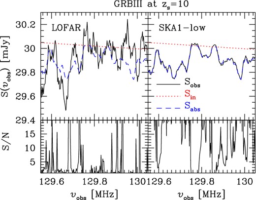
Upper panels: spectrum of a GRBIII positioned at z_s = 10 (i.e. ν ∼ 129 MHz), with a flux density S_in(z_s) = 30 mJy. The red dotted lines refer to the intrinsic spectrum of the source, S_in; the blue dashed lines to the simulated spectrum for 21 cm absorption, S_abs; and the black solid lines to the spectrum for 21 cm absorption as it would be seen with a bandwidth Δν = 10 kHz, after an integration time t_int = 1000 h. The left- and right-hand panels refer to a case with the noise σ_n given in equation (2) (LOFAR telescope) and with 0.1n (expected for SKA1-low), respectively. Lower panels: S/N corresponding to the upper panels. See text for further details.

Open in new tab Download slide

Fig. 2 shows a LOS to the same GRB located at z = 7.6, when the IGM is ∼80 per cent ionized by volume. The LOS has been chosen to intercept a pocket of gas with τ_21cm > 0.1 to show that strong absorption features could be detected, albeit by LOFAR only marginally with a S/N of a few, also at a redshift when most of the IGM is in a highly ionized state.

Figure 2.

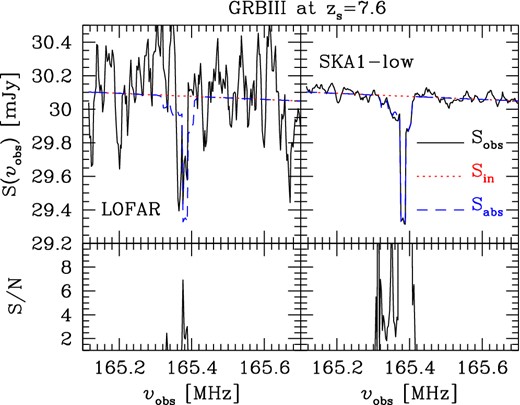
As Fig. 1, but the GRBIII is positioned at z_s = 7.6 (i.e. ν ∼ 165 MHz) and Δν = 5 kHz.

Open in new tab Download slide

On the other hand, a strong average absorption (rather than the absorption features seen in the previous figures) can be easily detected (S/N >10) in the spectra of GRBs located at very high redshift, as shown in Fig. 3. If the intrinsic spectrum of the source could be inferred through other means, for example, accurate spectral measurements of the unabsorbed continuum at GHz frequencies and above, such detection could be used to infer the global amount of neutral hydrogen present in the IGM.

Figure 3.

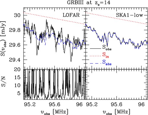
As Fig. 1, but the GRBIII is positioned at z_s = 14 (i.e. ν ∼ 95 MHz) and Δν = 20 kHz. Note that the S/N in the lower-right panel is always higher than the range covered by the axis.

Open in new tab Download slide

We have applied the same pipeline also to more standard GRBII, which have a flux density two to three orders of magnitude lower than a GRBIII. In this case we find that, even if we could collect 1000 h of observations with a noise 0.01 σ_n (i.e. 1/10th of the SKA1-low noise), these would be barely enough to detect absorption features in 21 cm. Also in the most optimistic case, with S_in(z_s) = 0.1 mJy, a positive detection would be extremely difficult at any redshift, as shown in Fig. 4, and only at z ≳ 9 a S/N larger than a few could be reached.

Figure 4.

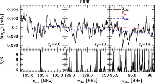
Upper panels: spectrum of a GRBII with a flux density S_in(z_s) = 0.1 mJy. The red dotted lines refer to the intrinsic spectrum of the source, S_in; the blue dashed lines to the simulated spectrum for 21 cm absorption, S_abs; and the black solid lines to the spectrum for 21 cm absorption as it would be seen after an integration time t_int = 1000 h with a noise 0.01 σ_n (i.e. 1/10th of the SKA1-low noise). The panels refer to a case with z_s = 7.6 and Δν = 5 kHz (left), z_s = 10 and Δν = 10 kHz (middle), z_s = 14 and Δν = 20 kHz (right). Lower panels: S/N corresponding to the upper panels. See text for further details.

Open in new tab Download slide

5 CONCLUSIONS

In this paper, we have discussed the feasibility of detecting 21 cm absorption features in the spectra of high redshift GRBs with LOFAR and SKA. The distribution of H i, gas temperature and velocity field used to calculate the optical depth to the 21 cm line have been obtained from the simulations of reionization presented in Ciardi et al. (2012) and C2013. We find that

absorption features in the spectra of highly energetic GRBs from Pop III stars could be marginally (with a S/N larger than a few, depending on redshift) detected by LOFAR at z ≳ 7;
the same features could be easily detected if the noise were reduced by one order of magnitude (similar to what is expected for SKA1-low);
the flux density of a more standard GRB is too low for absorption features to be detected even with ten times the sensitivity of SKA1-low. Only in the most optimistic case with a flux density of 0.1 mJy, can a S/N larger than a few be reached at z ≳ 9.

The problem of a small flux could be alleviated in case of a lensed GRB. Lensing of high-z sources has been already discussed in the literature both from a theoretical (e.g. Wyithe et al. 2011), and an observational (e.g. with the Frontier Fields as in Oesch et al. 2014) perspective. Alternatively, a statistical detection of the 21 cm forest could be attempted, as already suggested by several authors (e.g. Meiksin 2011; Mack & Wyithe 2012; Ewall-Wice et al. 2014).

The authors thank an anonymous referee for his/her useful comments. BC acknowledges Benoit Semelin for interesting discussions. This work was supported by DFG Priority Programs 1177 and 1573. SI appreciates support from Grant-in-Aid for Scientific Research No. 24340048 from MEXT of Japan. GH has received funding from the People Programme (Marie Curie Actions) of the European Union's Seventh Framework Programme (FP7/2007–2013) under REA grant agreement no. 327999. LVEK, HV, KA and AG acknowledge the financial support from the European Research Council under ERC-Starting Grant FIRSTLIGHT - 258942. ITI was supported by the Science and Technology Facilities Council [grant number ST/L000652/1]. VJ would like to thank the Netherlands Foundation for Scientific Research (NWO) for financial support through VENI grant 639.041.336. JSB acknowledges the support of a Royal Society University Research Fellowship.

1

http://lofar.org

2

http://www.mwatelescope.org

3

http://eor.berkeley.edu

4

http://www.skatelescope.org

5

http://www.almaobservatory.org/

6

We note that equation (2) is correct as long as the SEFD is calculated theoretically for a single polarization using the system temperature (as done in this paper), while when the SEFD is determined observationally from Stokes I the noise is reduced by a factor of sqrt(2), since it combines the two cross-dipole sensitivities.

7

Note that the same expression in C2013 contains a typo.

8

We note that the values obtained from equation (3) are very similar to the real ones reported in the LOFAR official webpage.

9

Although the time evolution after the jet break is not explicitly described in Inoue (2004), it is taken into account following Sari et al. (1999).

10

SKA1-low is the first phase of the SKA covering the lowest frequency band.

11

We note that the definition of ‘average’ is somewhat arbitrary and depends on the frequency range used. Here, the average refers to the one calculated over the frequency range shown in the Figures.

REFERENCES

Baek

S.

Di Matteo

P.

Semelin

B.

Combes

F.

Revaz

Y.

A&A

2009

495

389

Month:	Total Views:
February 2017	4
April 2017	4
May 2017	4
June 2017	3
July 2017	6
August 2017	3
September 2017	1
January 2018	3
February 2018	5
March 2018	3
May 2018	5
June 2018	5
July 2018	8
August 2018	1
September 2018	4
October 2018	14
November 2018	5
December 2018	11
January 2019	13
February 2019	4
March 2019	5
April 2019	8
May 2019	14
June 2019	8
July 2019	18
August 2019	14
September 2019	18
October 2019	40
November 2019	24
December 2019	9
January 2020	15
February 2020	14
March 2020	31
April 2020	10
May 2020	15
June 2020	9
July 2020	21
August 2020	15
September 2020	2
October 2020	8

Article Contents

Simulating the 21 cm forest detectable with LOFAR and SKA in the spectra of high-z GRBs Free

Abstract

1 INTRODUCTION

2 THE 21 cm FOREST

3 RADIO AFTERGLOWS OF HIGH-Z GRBs

4 RESULTS

5 CONCLUSIONS

REFERENCES

Citations

Views

Altmetric

Email alerts

Astrophysics Data System

Citing articles via

Latest

Most Read

Most Cited

This Feature Is Available To Subscribers Only

Simulating the 21 cm forest detectable with LOFAR and SKA in the spectra of high-z GRBs