Large-scale structure and integrated Sachs–Wolfe effect in decaying vacuum cosmology

Velten, H.; Borges, H. A.; Carneiro, S.; Fazolo, R.; Gomes, S.

doi:10.1093/mnras/stv1443

Abstract

The concordance particle creation model – a class of Λ(t) Cold Dark Matter (CDM) cosmologies – is studied using large-scale structure (LSS) formation, with particular attention to the integrated Sachs–Wolfe effect. The evolution of the gravitational potential and the amplitude of the cross-correlation of the cosmic microwave background (CMB) signal with LSS surveys are calculated in detail. We properly include in our analysis the peculiarities involving the baryonic dynamics of the Λ(t)CDM model which were not included in previous works. Although both the Λ(t)CDM and the standard cosmology are in agreement with available data for the CMB–LSS correlation, the former presents a slightly higher signal which can be identified with future data.

dark energy, dark matter

INTRODUCTION

Although the great success of the standard ΛCDM cosmological model in describing most observations, we are still distant from the full understanding of the cosmic dynamics. Apart from the so-called small-scale problems in the dark matter sector, there is also a huge discussion about dark energy properties. At the same time, the efficient approach given by a cosmological constant Λ still seems to face some challenges, mainly from the theoretical point of view.

Among the viable alternatives, it has been argued that a model with the mechanism of dark matter particle production at a constant rate Γ (implying in a dynamical vacuum term Λ(t)) is also capable to produce a concordance model (Alcaniz et al. 2012), although with a larger current matter fraction Ω_m0 ≈ 0.45.¹

If the total energy is given by ρ = ρ_m + Λ and the pressure of the vacuum contribution sets to p_Λ = −Λ, a constant Γ is equivalent to take Λ = 2ΓH, where |$H=\dot{a}/a$| is the Hubble rate.² Taking today's values one finds Γ = 3Ω_Λ0H₀/2. The matter dynamics corresponds to the balance

\begin{equation} \dot{\rho }_{{\rm m}}+3H\rho _{\rm m}=-\dot{\Lambda }, \end{equation}

(1)

from which it is not difficult to show that |$\dot{\Lambda }=-\Gamma \rho _{{\rm m}}$|⁠. The background expansion is given by

\begin{equation} H=H_0 \left( 1-\Omega _{{\rm m}0}+\Omega _{{\rm m}0}a^{-3/2}\right), \end{equation}

(2)

from which we can derive the matter density evolution

\begin{equation} \rho _{\rm m} =3H_0^2 \left[ \Omega _{{\rm m}0}^2 a^{-3}+(1 - \Omega _{{\rm m}0}) \Omega _{{\rm m}0}a^{-3/2}\right]. \end{equation}

(3)

Note that, as in the flat ΛCDM model, there are here also only two free parameters. The concordance of this Λ(t) cosmology with Ω_m0 ≈ 0.45 has been verified via many different observational data at both the background (Velten, Montiel & Carneiro 2005; Carneiro et al. 2006, 2008; Pigozzo et al. 2011) and perturbative (Zimdahl et al. 2011; Alcaniz et al. 2012; Devi et al. 2015) levels.

Concerning structure formation, the full cosmic microwave background (CMB) spectrum has not yet been obtained for this model, but CMB physics can also be accessed via integrated Sachs–Wolfe (ISW) studies, i.e. how time-varying gravitational potential wells change the temperature of the CMB photons as they cross structures (Sachs et al. 1967). The expansion of an Einstein–de Sitter universe compensates the clustering of structures, producing no ISW effect, i.e. in a matter dominated universe there is no ‘late time’ ISW effect.³ Dark energy modifies the background expansion and leads to a net contribution to (ΔT/T)^ISW. Then, it is expected that the modified background and perturbative expansion of the Λ(t)CDM model leaves a distinct imprint on the ISW signal.

Since the ISW is a secondary CMB temperature effect its detection occurs only via the cross-correlation with other large-scale probes like galaxies and quasars surveys (Crittenden et al. 2005). Wang et al. (2010) used the cross-correlation technique to probe the Λ(t)CDM model, finding an increase of the ISW-galaxy spectrum (⁠|$C^{Tg}_l$|⁠) in comparison to the ΛCDM model. Our aim in this paper is to perform this analysis taking care with some peculiarities of the model. In particular, it is important to differentiate the evolution of the baryonic and dark matter components. At the background level, baryons are included in the conserved part of equation (3). Concerning perturbations, the observed matter power spectrum P(k) = |δ(k)|² is a measurement of the baryonic clustering, which is sourced by the gravitational potential. In the ΛCDM model there is almost no difference between the evolution on large scales of such components. The same does not happen in the Λ(t)CDM model, where one observes a late-time suppression in the dark matter and total matter contrasts owing to dark matter production, a suppression not observed in the baryonic contrast.

Our interest is also justified by a possible tension between the theoretical ΛCDM predictions and the observed ISW signal. Some analysis have reported a cross-correlation signal 1σ–2σ above that expected in the standard cosmology (Giannantonio et al. 2008; Goto, Szapudi & Granett 2012, see Giannantonio et al. 2012 for a critical review on this issue). Recent studies claim a better statistical concordance though the observed signal is still higher than the theoretical one (Kovács et al. 2013; Ferraro, Sherwin & Spergel 2015). Also, the inferred stacking of CMB data on the position of superstructures is about five times larger than the ΛCDM prediction (Granett, Neyrinck & Szapudi 2008; Nadathur, Hotchkiss & Sarkar 2012; Flender, Hotchkiss & Nadathur 2013; Hernández-Monteagudoet & Smith 2013). This result has recently been confirmed by the 2015 release of the Planck CMB data (Planck Collaboration 2015).

In the next section we develop the background expansion which will be used in this paper. In Section 3 we explore the scalar perturbations of the model. The connection with the ISW effect is made via a direct calculation of the evolution of the gravitational potential (Section 3.2) and the ISW–LSS cross-correlation (Section 3.3). We conclude in the final section.

Λ(t) BACKGROUND DYNAMICS

The brief description of the Λ(t)CDM dynamics given in equations (1)–(3) has been widely derived in the literature (see Alcaniz et al. 2012 and references therein). Note that as in the standard case the important quantity is the total matter density Ω_m0, the sum of the dark matter Ω_dm0 and baryons Ω_b0. The latter is constrained by nucleosynthesis and is well approximated by Ω_b0 = 0.05. We assume hereafter this value. The baryonic sector is conserved and therefore we have the continuity equations

\begin{equation} \dot{\rho }_{{\rm dm}}+3H\rho _{{\rm dm}}=-\dot{\Lambda } \end{equation}

(4)

and

\begin{equation} \dot{\rho }_{{\rm b}}+3H\rho _{\rm b}=0. \end{equation}

(5)

Adding these equations we obtain the total matter conservation equation (1). With Λ = 2ΓH, the dynamics presented in Section 1 follows. That is, the background expansion is obtained after solving the system given by the continuity equation

\begin{equation} aH\rho ^{\prime }_{{\rm m}}+3H \rho _{{\rm m}}=\Gamma \rho _{{\rm m}} \end{equation}

(6)

and the Friedmann equation

\begin{equation} 2aHH^{\prime } + \rho _{{\rm m}}=0, \end{equation}

(7)

where the prime means derivative with respect to the scale factor.

PERTURBATIVE DYNAMICS

Growth functions

When cosmological perturbation theory is used to study the large-scale structure (LSS) of the universe we are most interested in the evolution of scalar quantities like the density contrast and the gravitational potential. The Λ(t)CDM models have the particularity of suppressing the growth of dark matter contrast δ_dm. However, the observed structures reflect the behaviour of the baryonic contrast, δ_b = δρ_b/ρ_b, instead. In the standard cosmology this quantity coincides with the dark matter contrast, and the total matter contrast δ_m denotes both behaviours. For the Λ(t)CDM model, however, we should make a distinction between the different components. Using the fact that the vacuum fluctuations are negligible (Zimdahl et al. 2011) and choosing the comoving synchronous gauge we obtain the set of equations⁴

\begin{equation} \dot{\delta }_{{\rm m}}+{\Gamma }\delta _{{\rm m}}=\frac{\dot{h}}{2}, \end{equation}

(8)

\begin{equation} \dot{\delta }_{{\rm b}}=\frac{\dot{h}}{2}, \end{equation}

(9)

\begin{equation} \ddot{h}+2H\dot{h}=\rho _{{\rm m}} \delta _{{\rm m}}, \end{equation}

(10)

where h is the trace of the spatial metric perturbation. Combining these equations and changing to the derivative with respect to the scale factor we find

\begin{eqnarray} &&{a^2H^2 \delta ^{\prime \prime }_{{\rm m}}+aH(3H+aH^{\prime }+{\Gamma })\delta ^{\prime }_{{\rm m}}} \nonumber \\ &&{\quad+\,2{\Gamma } H \delta _{{\rm m}} = \frac{1}{2} \rho _{{\rm m}} \delta _{{\rm m}}} \end{eqnarray}

(11)

and

\begin{eqnarray} a^2H^2 \delta ^{\prime \prime }_{{\rm b}}+aH(3H+aH^{\prime })\delta ^{\prime }_{{\rm b}} =\frac{1}{2}\rho _{{\rm m}} \delta _{{\rm m}}. \end{eqnarray}

(12)

In Fig. 1 we plot the evolution of the density contrasts as calculated in equations (11) and (12). For the ΛCDM model (black curves) we set Ω_m0 = 0.23, the best fit of LSS observations (Cole et al. 2005; Percival et al. 2007).⁵ We show the Λ(t)CDM evolutions for δ_b and δ_m in the solid red and dashed red curves, respectively. We have used initial conditions δ_b(a = 0.001) = δ_m(a = 0.001) = 10⁻⁵ and |$\delta ^{\prime }_{{\rm b}}(a=0.001)=\delta ^{\prime }_{{\rm m}}(a=0.001)=0$|⁠. As expected, δ_b and δ_m have the same evolution in the standard case. On the other hand, the plot shows a late-time growth suppression of δ_m in the Λ(t)CDM model, a consequence of dark matter creation. The same suppression is not observed in the baryonic contrast, though its amplitude achieves a plateau on late times which is slightly below the standard scenario.

Figure 1.

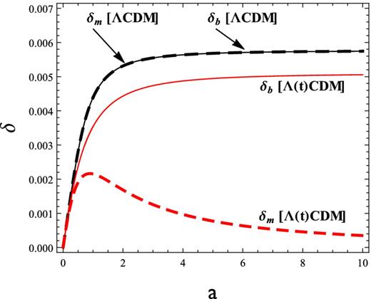
Evolution of the linear density contrasts. The black curves correspond to the baryonic (solid black curve) growth and total matter (dashed black curve) growth for the ΛCDM model with Ω_m0 = 0.23. Related plots for the Λ(t)CDM with Ω_m0 = 0.45 are in solid red (baryons) and dashed red (total matter), respectively.

Open in new tab Download slide

Evolution of the gravitational potential

The evolution of the gravitational potential Φ determines the ISW contribution to the total CMB spectrum via the formula

\begin{equation} \frac{\Delta T}{T}^{\rm ISW} = 2\int ^{1}_{a_{\rm d}} \frac{\mathrm{\partial} \Phi }{\mathrm{\partial} a} {\rm d}a, \end{equation}

(13)

where the subscript ‘d’ denotes the decoupling time and a = 1 at present. Writing down the Poisson equation in the comoving synchronous gauge we find

\begin{equation} k^2 \Phi = - \frac{a^2}{2}\rho _{{\rm m}}\delta _{{\rm m}}, \end{equation}

(14)

where k is the comoving wavenumber. This expression allows us to calculate the ISW, which can be computed via the line-of-sight integration (13). It is useful to perform it in terms of the comoving distance

\begin{equation} \chi (a)=\int ^1_a \frac{{\rm d}a}{a^2 H(a)}. \end{equation}

(15)

The ISW then reads

\begin{eqnarray} \frac{\Delta T}{T}^{\rm ISW}=\frac{\delta _{{\rm m}}(a=1)}{k^2}\int ^{\chi _{\rm d}}_0 a^2 H(a) \frac{{\rm d}Q_{{\rm m}} (a)}{{\rm d}a} {\rm d}\chi , \end{eqnarray}

(16)

where we have defined

\begin{eqnarray} Q_{{\rm m}}(a) &=& a^2 \rho _{{\rm m}}(a) D^+_{{\rm m}}(a), \end{eqnarray}

(17)

with

\begin{eqnarray} D^+_{{\rm m}}(a) &=& \frac{\delta _{\rm m}(a)}{\delta _{{\rm m}}(a=1)}. \end{eqnarray}

(18)

The baryonic and total matter density contrasts can be directly calculated from the solution of equations (11) and (12). Using equation (14), we compare in Fig. 2 the predictions for the ΛCDM and Λ(t)CDM gravitational potentials as functions of the redshift z. We access the observational predictions for the ISW effect via the cross-correlation of CMB maps and LSS surveys, to be done in next section.

Figure 2.

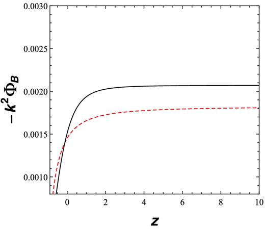
Evolution of the gravitational potential for the ΛCDM model with Ω_m0 = 0.23 (black) and for the Λ(t)CDM with Ω_m0 = 0.45 (red dashed).

Open in new tab Download slide

Correlating CMB maps and galaxy surveys

In order to compute the cross-correlation between CMB and LSS we also need to describe the evolution of the observed galaxy contrast δ_g on the line of sight. This quantity depends on the survey design and is obtained from

\begin{equation} \delta _{\rm g} = \int ^{\chi _{\rm d}}_0 b(z) \frac{{\rm d}N}{{\rm d}z} H(a) \delta _{{\rm b}}(a)\, {\rm d}\chi , \end{equation}

(19)

where δ_b is the baryonic linear contrast and b(z) is the standard bias between δ_g and δ_b.⁶

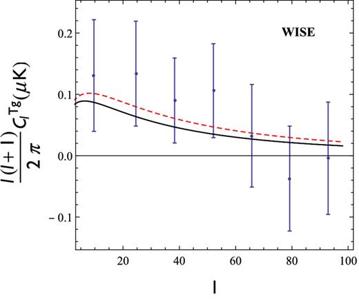
The redshift distribution of the observed galaxy sample is a model-independent quantity. Each survey has its own dN/dz histogram function. We use in this work data from the NRAO VLA Sky Survey (NVSS)⁷ and the Wide-field Infrared Survey Explorer (WISE)⁸ catalogues. Both surveys are widely used for cross-correlation studies. The NVSS covers the entire north sky of −40 deg declination in one band. The produced catalogue of discrete sources contains more than one million objects. Full details appear in Condon et al. (1998). WISE has an entire sky scanning strategy in four frequency bands. It has an average redshift 0.3, but reaching up to z ∼ 1, collecting about 500 million sources which are in general not restricted to point-like objects such as stars and unresolved galaxies. The data used in this work are taken from the analysis recently performed in Ferraro et al. (2015) which uses a larger sample by applying less-conservative cuts to the data set in comparison to previous works (Goto et al. 2012; Kovács et al. 2013).

For the NVSS catalogue one has

\begin{equation} b(z)\frac{{\rm d}N}{{\rm d}z}=b_{\rm eff}\frac{\alpha ^{\alpha +1}}{z_{\star }^{\alpha +1}\Gamma (\alpha )}z^{\alpha } {\rm exp} \left[-\frac{\alpha z}{z_{\star }}\right], \end{equation}

(20)

where the values b_eff = 1.98, z_⋆ = 0.79 and α = 1.18 were fitted in Ho et al. (2008). For the WISE catalogue dN/dz can be obtained numerically from Yan et al. (2010) and, following Ferraro et al. (2015), we adopt a constant bias b(z) = 1.41. We will limit our results to constant bias models since the use of time-dependent b(z) bias will not change our main conclusion.

Combining equations (16) and (19), the multipole coefficients for the cross-correlation spectrum are given by

\begin{equation} C_{Tg}(l) = \int ^{a_d}_{1} \frac{W_T (a)\, W_g (a)}{a^2 H(a)} \frac{P(k=l/\chi )}{l^2} {\rm d}a, \end{equation}

(21)

where we have defined the weight functions

\begin{eqnarray} W_T\,(a) &=& a^2 H(a) \frac{{\rm d}Q(a)}{{\rm d}a}, \end{eqnarray}

(22)

\begin{eqnarray} W_g\,(a) &=& H(a) b(z)\frac{{\rm d}N}{{\rm d}z} D^+_{\rm b}(a), \end{eqnarray}

(23)

with

\begin{equation} D^+_{\rm b}(a) = \frac{\delta _{\rm b}(a)}{\delta _{\rm b}(a=1)}. \end{equation}

(24)

We have also defined the crossed power spectrum

\begin{equation} P(k) = \frac{\delta _{\rm m}(a=1)}{\delta _{\rm b}(a=1)} P_{\rm b}(k), \end{equation}

(25)

where P_b(k) is the observed baryonic spectrum, given by

\begin{equation} P_{\rm b}(k) = P_0 k^{n_{\rm s}} T^2(k), \end{equation}

(26)

where P₀ is a normalization constant determined from observations (Alcaniz et al. 2012). This normalization constant is not the same as in the ΛCDM model as can be seen by an inspection of Figs 1 and 2. It can also be determined by writing |$P_0 \delta _{\rm b}^2(1) = \bar{P}_0 \bar{\delta }_{\rm b}^2(1)$|⁠, where the barred quantities are the standard ones (Devi et al. 2015). For T(k) we will use the BBKS transfer function (Barden et al. 1986; Martin, Riazuelo & Sakellariadou 2000) which, for Ω_b0 ≪ Ω_m0, can be approximated by

\begin{eqnarray} T(x&=&k/k_{\rm eq})=\frac{{\rm ln}[1+0.171x]}{(0.171x)} \nonumber \\ &&\times \left[1 + 0.284x + (1.18x)^2 + (0.399x)^3 + (0.490x)^4\right]^{-0.25}.\nonumber\\ \end{eqnarray}

(27)

Here, |$k_{\rm eq}^{-1}$| is the comoving Hubble radius at the time of matter–radiation equality. From equation (3) it is easy to show that it is given by (Alcaniz et al. 2012; Devi et al. 2015) |$k_{\rm eq} = 0.073 \, h^2 \Omega _{\rm m0}^2$| Mpc⁻¹, where, here, h = H₀/(100 km s⁻¹ Mpc) and we have set the present radiation density as Ω_R0 = 4.15 × 10⁻⁵h⁻². We will adopt h = 0.7 and n_s = 1.

The resulting cross-correlation spectrum is show in Figs 3 and 4. For the NVSS data (Fig. 3) we follow the presentation of data used in Wang et al. (2010), where the original data points of Ho et al. (2008) located at l < 10 and l > 70 have been removed due to their high dispersion. The WISE data presented in Fig. 4 are taken from Ferraro et al. (2015). In both cases, the |$C^{Tg}_l$| spectrum for the Λ(t)CDM model presents a slightly larger signal as compared to the standard model. This seems to be a virtue of the particle creation model since we have learned from previous studies (Grannett et al. 2008; Giannantonio et al. 2012; Nadathur et al. 2012; Kovács et al. 2013; Flender et al. 2013; Hernández-Monteagudoet & Smith 2013; Ferraro et al. 2015) that models with higher |$C^{Tg}_l$| power are desirable. Nevertheless, given the large uncertainties in determining the observed |$C^{Tg}_l$| values, both models remain compatible with data.

Figure 3.

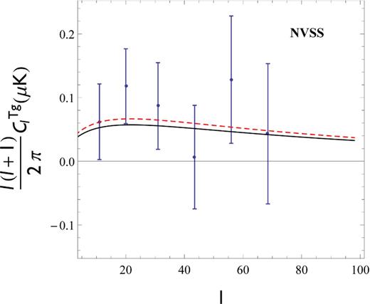
CMB-LSS cross-correlation spectrum using the NVSS data taken from Ho et al. (2008, see text for details). The black line represents the ΛCDM with Ω_m0 = 0.23. The red dashed line is our inferred spectrum for the Λ(t)CDM model using Ω_m0 = 0.45.

Open in new tab Download slide

Figure 4.

The same as Fig. 3 for the WISE data taken from Ferraro et al. (2015).

Open in new tab Download slide

CONCLUSIONS

The concordance particle creation model is a viable alternative to the standard ΛCDM paradigm, with the same free parameters, namely Ω_m0 and H₀. Since particle creation at a constant rate leads to a different background and perturbative dynamics, it is important to investigate specific signatures of this model in comparison to the standard cosmology. We provided in this work a direct computation of the evolution of perturbed scalar quantities like the matter and baryonic density contrasts and the gravitational potential for the Λ(t)CDM model. There is a clear scenario emerging in such a cosmology (see Fig. 1), in which the dark matter contrast is highly suppressed at late times while the baryonic contrast maintains a constant value, as in the standard case, but with a slightly smaller amplitude. This dynamics does indeed lead to a consistent description of the structure formation data (Zimdahl et al. 2011; Alcaniz et al. 2012; Devi et al. 2015). Our main goal here was to provide a comprehensive analysis of the ISW effect in such concordance particle creation cosmology. With the results for the perturbative dynamics calculated in Section 3 we computed the CMB–LSS cross-correlation spectrum. Our care in calculating the evolution of both baryonic and total matter contrasts in detail leads to a full and safe analysis of the |$C^{Tg}_l$| spectrum.

Current efforts (Grannett et al. 2008; Giannantonio et al. 2012; Nadathur et al. 2012; Kovács et al. 2013; Flender et al. 2013; Hernández-Monteagudoet & Smith 2013; Ferraro et al. 2015) in obtaining the observed |$C^{Tg}_l$| spectrum are sending a clear message: the CMB–LSS signal seems to slightly exceed the ΛCDM prediction. Therefore, it is timely to check the Λ(t)CDM outcomes for this cosmological observable. For both the NVSS (Fig. 3) and WISE (Fig. 4) data, the Λ(t)CDM model leads to a desirable excess of power in the |$C^{Tg}_l$| spectrum of the order of 10–20 per cent. This is in fact a small increase that potentially cannot be sensitive to ISW probes. It is worth noting that the available data are insufficient for distinguishing cosmological models with a reliable statistical confidence. This happens mainly because of the cosmic variance limits imposed to large-scale CMB analysis, that leads to a very low signal-to-noise ratio. Here we are restricted to a qualitative comparison between the Λ(t) and standard cosmologies. Future data can in principle improve the accuracy of the CMB–LSS cross-correlation technique and therefore specific features of different cosmological models concerning the ISW effect could be compared in more detail. Although pure ISW detection techniques do not seem to be a powerful tool in discriminating cosmological models, they can eventually complement other cosmological probes.

We are thankful to Wang et al. (2010) for making their code available and to J. Enander, S. Ilic and C. Pigozzo for helpful discussions. HAB thanks the partial support of CNPq (Brazil), through the ‘Science without Border’ programme, and Fapesb. SC thanks the partial support of CNPq, grants no. 309792/2014–2 and 479937/2013–3. HV acknowledges CNPq and support of A*MIDEX project (no. ANR-11-IDEX-0001-02) funded by the ‘Investissements d'avenir’ French Government programme, managed by the French National Research Agency (ANR). The work of RF and SG is funded by CNPq.

1

For any component i we define Ω_i = ρ_i/ρ_c0 with |$\rho _{c0}=3 H^2_0 / 8\pi G$|⁠, where the subscript 0 denotes today's values. In this paper we will take 8πG = c = 1.

2

Strictly speaking, this equivalence is only valid if we neglect the conserved baryons in the background equations. In the presence of a small baryonic content, taking Λ ∝ H does not lead to an exactly constant Γ.

3

The ‘early time’ ISW effect is related to non-insignificant radiation density just after photon decoupling.

4

A different approach to the baryonic sector can be found in Zimdahl et al. (2014).

5

Using, instead, the ΛCDM concordance value Ω_m0 = 0.27 does not change significantly our final results.

6

In the ΛCDM, model is irrespective to use δ_b or δ_m in equation (19), but the same is not true for the Λ(t) case, as can be seen in Fig. 1.

7

http://www.cv.nrao.edu/nvss/

8

http://wise.ssl.berkeley.edu/

REFERENCES

Alcaniz

J. S.

Borges

H. A.

Carneiro

S.

Fabris

J. C.

Pigozzo

C.

Zimdahl

W.

Phys. Lett. B

2012

716

165

Month:	Total Views:
February 2017	4
March 2017	2
May 2017	3
June 2017	1
August 2017	1
September 2017	2
December 2017	2
March 2018	1
May 2018	10
August 2018	4
September 2018	3
October 2018	3
November 2018	4
December 2018	1
January 2019	2
February 2019	1
March 2019	5
April 2019	9
May 2019	5
June 2019	5
July 2019	5
August 2019	12
September 2019	3
October 2019	20
November 2019	11
December 2019	5
January 2020	12
February 2020	2
March 2020	6
April 2020	5
May 2020	4
June 2020	3
July 2020	3
August 2020	4
September 2020	4
October 2020	1
November 2020	2
December 2020	1
January 2021	4
February 2021	5

Article Contents

Large-scale structure and integrated Sachs–Wolfe effect in decaying vacuum cosmology Free

Abstract

INTRODUCTION

Λ(t) BACKGROUND DYNAMICS

PERTURBATIVE DYNAMICS

Growth functions

Evolution of the gravitational potential

Correlating CMB maps and galaxy surveys

CONCLUSIONS

REFERENCES

Citations

Views

Altmetric

Email alerts

Astrophysics Data System

Citing articles via

Latest

Most Read

Most Cited

This Feature Is Available To Subscribers Only

Large-scale structure and integrated Sachs–Wolfe effect in decaying vacuum cosmology