


Abstract
It is shown here that in a flat, cold dark matter (CDM)-dominated Universe with positive cosmological constant (Λ), modelled in terms of a Newtonian and collisionless fluid, particle trajectories are analytical in time (representable by a convergent Taylor series) until at least a finite time after decoupling. The time variable used for this statement is the cosmic scale factor, i.e. the ‘a-time’, and not the cosmic time. For this, a Lagrangian-coordinate formulation of the Euler–Poisson equations is employed, originally used by Cauchy for 3D incompressible flow. Temporal analyticity for ΛCDM is found to be a consequence of novel explicit all-order recursion relations for the a-time Taylor coefficients of the Lagrangian displacement field, from which we derive the convergence of the a-time Taylor series. A lower bound for the a-time where analyticity is guaranteed and shell-crossing is ruled out is obtained, whose value depends only on Λ and on the initial spatial smoothness of the density field. The largest time interval is achieved when Λ vanishes, i.e. for an Einstein–de Sitter universe. Analyticity holds also if, instead of the a-time, one uses the linear structure growth D-time, but no simple recursion relations are then obtained. The analyticity result also holds when a curvature term is included in the Friedmann equation for the background, but inclusion of a radiation term arising from the primordial era spoils analyticity.
INTRODUCTION
Recent observational results (Planck Collaboration XVI 2014) indicate that we live in a spatially flat ΛCDM Universe which is nowadays dominated by a cold dark matter (CDM) component and a cosmological constant, Λ > 0. In a primordial era, matter was tightly coupled to radiation via electroweak interactions. This tight coupling prevented matter to cluster significantly at early times since the radiation pressure acted as a counter force to the gravitational force. As the Universe expands its mean energy density decreases, which eventually lead to a freeze-out of these electroweak interactions. This freeze-out of the interactions (non-instantaneous in space and time) happened roughly 380 000 yr after the big bang, eventually enabling the matter to cluster. This epoch, usually called decoupling or recombination, marks the beginning of cosmological structure formation with initially smooth matter density fluctuations.
The observed large-scale structure of the Universe is mainly the result of the gravitational instability. To study the structure formation, it is usually assumed that the CDM component behaves as a Newtonian pressureless and curl-free fluid (so-called cosmological dust). Such a fluid is governed by the Euler–Poisson equations, together with the Friedmann equation, where the latter describes the background evolution of the expanding Universe. Since that background evolution is by definition exactly homogeneous and isotropic, it is parametrized by a single function (of cosmic time t): the cosmic scale factor a(t).
Analytical models for cosmological structure formation can be formulated in either the Eulerian or Lagrangian frame of reference (for some reviews, see e.g. Bernardeau et al. 2002; Bernardeau 2015). The class of analytical models of the latter is dubbed the Lagrangian perturbation theory (LPT; Buchert & Goetz 1987; Buchert 1989, 1992; Bildhauer, Buchert & Kasai 1992; Bouchet et al. 1992, 1995; Catelan 1995; Ehlers & Buchert 1997). When using this technique, the only dynamical variable is the displacement, which represents the gravitationally induced deviation of the particle trajectory field from the homogeneous background evolution of the Universe. To solve the Euler–Poisson equations in Lagrangian space, one usually requires some power series Ansatz for the displacement (for more information, see also below in the Introduction).
The LPT is widely applied in cosmology. Buchert (1992) showed that the Zel'dovich approximation (Zel'dovich 1970) is actually an instance of the first-order LPT (see also Novikov 1970). Simply and elegantly, it quite well describes the gravitational evolution of CDM inhomogeneities, as long as the trajectories of fluid particles do not cross. A Lagrangian approach has been also used in the so-called cosmological reconstruction problem in an expanding Universe (Frisch et al. 2002; Brenier et al. 2003), where it is shown that, in so far as the dynamics are governed by the Euler–Poisson equations, the knowledge of both the present highly non-uniform distribution of mass and of its primordial quasi-uniform distribution, uniquely determines the inverse Lagrangian map, defined as the transformation from present Eulerian positions to their respective initial positions. The LPT is also an important tool in numerical investigations. In recent years, second-order LPT (2LPT) has been successfully used to set up initial conditions for numerical N-body simulations (see e.g. Crocce, Pueblas & Scoccimarro 2006). The so-called biasing model, whose task is to find a relationship between the visible matter and the dark matter distribution, yields good predictions to cosmological observations when formulated in Lagrangian space (Mo & White 1996; Matsubara 2008b). Also, semi-analytical approaches to LPT deliver statistical estimators, such as the matter power spectrum and bispectrum, which compare favourably with results from N-body simulations (e.g. Matsubara 2008a; Rampf & Wong 2012; Vlah, Seljak & Baldauf 2014). These approaches make use of the LPT up to the fourth order (Rampf 2012; Rampf & Buchert 2012). Most of the LPT calculations are performed for a flat CDM universe with vanishing cosmological constant, i.e. for an Einstein–de Sitter (EdS) universe, and only few investigations, up to the third order, are known for a ΛCDM Universe (see, e.g. Matsubara 1995; Lee 2014). The LPT has also been generalized to General Relativity, for a non-perturbative formulation see Buchert & Ostermann (2012) and Buchert, Nayet & Wiegand (2013). For a general relativistic treatment within the ΛCDM model, see Rampf & Rigopoulos (2013), Rampf (2013) and Rampf & Wiegand (2014).
Although LPT is widely applied in cosmology, very little is known about its convergence properties, which requires some knowledge about terms of arbitrarily high order. There are of course some exceptions; for example, Sahni & Shandarin (1996) investigated the case of an initial ‘top-hat underdensity’ that is initially discontinuous, and found that low-order perturbation worked better than a higher order one, which they regarded as a possible evidence for ‘semiconvergence’ of the perturbation series (see also Moutarde et al. 1991). Recently, a novel Lagrangian-coordinate approach has been used to show that particle trajectories for an EdS universe are time analytical until a finite time (Zheligovsky & Frisch 2014). Their approach is based on a little known Lagrangian formulation of ideal fluid flow derived by Cauchy in 1815 (Frisch & Villone 2014). In this paper, we show that the approach of Zheligovsky & Frisch (2014) can be extended to a ΛCDM Universe (and even beyond, see below), derive novel recursion relations and prove time analyticity in the cosmic scale factor time, here used both as a time variable and as an expansion parameter.
In the LPT literature, analytical results for ΛCDM usually employ an expansion in powers of small displacements, which amounts to performing a (Taylor) expansion in powers of the initial peculiar gravitational potential, |$\varphi _g^{\rm (init)} \sim 10^{-5}$|. By this technique, one seeks (reasonably well) approximate solutions of the non-linear Euler–Poisson equations. As a consequence of such an approximation technique, one is forced to solve at each order in perturbation theory a second-order partial differential equation for the time coefficient of the displacement (the fastest growing solutions of these time coefficients are usually denoted with D(t), E(t), etc.). Because of that it is impossible to obtain recursion relations for ΛCDM by the use of such a ‘small displacement’ expansion. In this paper, by contrast, we perform a time Taylor expansion and seek for exact analytic solutions for the fully non-linear Euler–Poisson equations in Lagrangian space. As a consequence of our expansion scheme, the displacement is represented in terms of a power series in the cosmic scale factor (even for a ΛCDM Universe!), and there is thus no need to explicitly solve partial differential equations (PDEs) for higher order time coefficients.
This paper is organized as follows. In Section 2, we present various forms of the Euler–Poisson equations in a Eulerian-coordinate system and we show that regularity of the solution at short times requires certain slaving constraints on the initial conditions. In Section 3, we turn to the Euler–Poisson equations in Lagrangian coordinates, which take a particularly simple form when using the cosmic scale factor as the time parameter. Recursion relations are derived in Section 4, from which time-analyticity is derived in Section 5. Further results related to time-analyticity are discussed in Section 6. This includes the dependence of the time of guaranteed analyticity on the cosmological constant Λ (Section 6.1), the absence of shell-crossing during the time interval where analyticity can be proved (Section 6.2), the analyticity in the linear growth time variable D (Section 6.3) and the persistence of analyticity when curvature effects are included, as well as the problem that arises with radiation effects (Section 6.4). Finally, in Section 7, we summarize our main findings and highlight various challenging open problems, such as using analyticity to develop a semi-Lagrangian numerical approach to the cosmological reconstruction.
THE VARIOUS FORMS OF THE EULER–POISSON EQUATIONS AND THE SLAVING CONDITIONS
Note that the peculiar Euler–Poisson equations depend on the comoving coordinate |$\boldsymbol {x} \equiv \boldsymbol {r}/a$|. Although these equations are indeed valid for a fluid model with cosmological constant, the latter does not explicitly appear in the peculiar approach, but only implicitly through Friedmann's background evolution equation (3).
The cosmic scale factor a, being dimensionless, is conveniently normalized to unity at the present-time epoch. At decoupling it then has a value of about 10−3. Here, we let the cosmic scale factor start at the value zero, while using the Euler–Poisson model with slaving. As a consequence, the whole primordial (pre-decoupling) cosmology is just reduced to the prescription of the slaving conditions (10). We shall come back to this issue in the Concluding Remarks (Section 7).
THE LAGRANGIAN FORMULATION OF ΛCDM
Time Taylor expansions can be carried out in either Eulerian or in Lagrangian coordinates. For such expansions to be convergent, i.e. for the radius of convergence not to vanish, it is much preferable to work in Lagrangian coordinates. Indeed, if the initial conditions have spatial derivatives only up to some finite order, the Eulerian solutions will have time derivatives only up to the same order. The reason is that, when one takes a time derivative in Eulerian coordinates, this generates a space derivative, because of the |$(\boldsymbol {v} \cdot {\nabla }_{\boldsymbol{x}}) \boldsymbol {v}$| term. Hence, time Taylor coefficients will not exist beyond that order. This does not happen in Lagrangian coordinates, where a limited amount of smoothness in the initial data suffices to ensure time-analyticity (Zheligovsky & Frisch 2014). Even when the initial data are spatially analytic, so that the solutions are time analytic in both Eulerian and Lagrangian coordinates, the Lagrangian radius of convergence, being controlled by the largest strain in the initial data, is typically much larger than the Eulerian one, which depends on the largest initial velocity present (for more details on such matters, see Podvigina, Zheligovsky & Frisch 2015).
THE FORMAL TAYLOR EXPANSION AND THE RECURSION RELATIONS
In the LPT literature, analytical derivations of results for ΛCDM usually rely on an expansion in powers of small displacements, which amounts to performing a power series expansion in the initial peculiar gravitational potential (see e.g. Matsubara 1995; Bernardeau et al. 2002). In this paper, we follow a different approach and perform an expansion in powers of a-time. Note that for the case of an EdS universe, one can obtain recursion relations for the displacement by both expansion techniques, and the resulting recursion relations are formally identical (Rampf 2012). For a ΛCDM Universe, however, explicit results for the displacement will generally differ depending on what expansion scheme is used.
THE TIME-ANALYTICITY OF THE LAGRANGIAN SOLUTION
Let us proceed now with the details. First, we observe that the r.h.s.'s of the recursion relations (26) for the gradient tensors are themselves mostly polynomials (of degree not exceeding three) of the lesser order gradient tensors. We write ‘mostly’ because there are also the Calderon–Zygmund operators, |${\cal C}_{ij}$|. In the present case, these operators stem from the non-local nature of the gravitational interaction. Technically speaking, these are pseudo-differential operators of degree zero (because an inverse Laplacian is compensated by two space derivatives). Essentially, such operators do not change the degree of differentiability of the functions they are applied to. But this is true only when using a suitable function space in which the Calderon–Zygmund operators are bounded.
Given the structure of the recursion relations (26) and using the boundedness of the Calderon–Zygmund operators and the algebra properties of the ℓ1 norm, it is elementary to show that if |${\nabla }^{\rm L}\boldsymbol {v}^{(\rm init)}$| is in the space ℓ1, so will be the gradients of the Taylor coefficients |${\nabla }^{\rm L}\boldsymbol {\xi }^{(s)}$|. The assumption that the gradient of the initial velocity has absolutely summable Fourier coefficients is the key hypothesis of the present work.
Knowing that all the (Lagrangian) gradients of the Taylor coefficients are in ℓ1 is not enough to ensure the convergence of the gradient Taylor series. For this, we need to obtain suitable bounds on the ℓ1 norms of |${\nabla }^{\rm L}\boldsymbol {\xi }^{(s)}$|, and then we need to show that these bounds imply the convergence of the gradient time Taylor series. Here we work with the time Taylor series for the spatial gradient of the displacement and establish its time-analyticity, from which follows the time-analyticity of the displacement (and also, of course, of the full Lagrangian map). To obtain the bounds on the ℓ1 norms, we shall mostly follow the approach presented in Zheligovsky & Frisch (2014). Of course, due to the presence of the cosmological constant, the third-order polynomials contain additional terms, and their study is more involved.
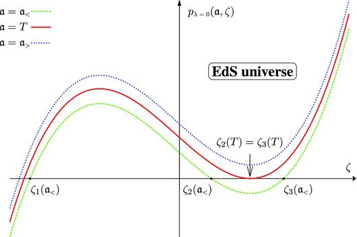
Sketch of the polynomial (36), for λ = 0, i.e. for the case of an EdS universe. Shown are three values of the rescaled time |$\mathfrak {a}$| for which |$0 < \mathfrak {a}_{{\rm <}} < T({\rm \lambda =0}) < \mathfrak {a}_{{\rm >}}$|, illustrating the behaviour of real roots of |$p_0(\mathfrak {a},\zeta )$| (the roots are shown as the points of intersection of the graph of |$p_{0}(\mathfrak {a}_{{\rm <}},\zeta )$| and the horizontal axis). On increasing |$\mathfrak {a}$|, the graph slides up as a rigid curve. As a result, the roots ζ1 and ζ3 move to the left (i.e. become smaller), whereas ζ2 moves to the right (i.e. becomes larger). At the critical value T(0), when ∂p0/∂ζ = 0 and the discriminant Δ vanishes, the two roots ζ2 and ζ3 collide and then disappear (with the emergence of a pair of complex conjugate roots).
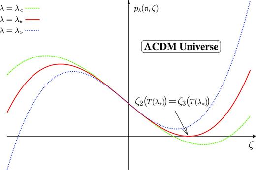
Sketch of the polynomial (36) for any fixed rescaled time variable |$\mathfrak {a}>0$| and λ ≠ 0 (i.e. the ΛCDM case). Three values of lambda are shown for which λ < < λ⋆ < λ >. The value λ⋆ denotes the critical value for which the cubic polynomial pλ develops a double root, i.e. where ζ2(T(λ)) = ζ3(T(λ)). In that case, the fixed value of the rescaled time |$\mathfrak {a}$| is precisely the critical value T(λ⋆) for which the generating function ζ of the displacement is bounded. On increasing λ for any fixed rescaled time |$\mathfrak {a} >0$|, the graph gets shifted into the upper left direction.
FURTHER RESULTS ON ANALYTICITY
The lower bound on the radius of analyticity and its dependence on the cosmological constant
The lowest positive root T(λ) of the discriminant equation (37) gives us a lower bound on the radius of analyticity of the time Taylor series for the Lagrangian map. This discriminant equation is of 12th degree in the rescaled time variable |$\mathfrak {a}= a \Vert {\nabla }^{\rm L} \boldsymbol {v}^{\rm (init)}\Vert$| and we have not been able to solve it explicitly by radicals. We can however solve the discriminant equation perturbatively for small and large rescaled cosmological constant |$\lambda = \Lambda / \Vert {\nabla }^{\rm L} \boldsymbol {v}^{\rm (init)}\Vert ^3$| and numerically for other values.
We have solved the discriminant equation (37) numerically for more than 100 values of λ, suitably distributed between 10−2 and 1014. The results are shown in Fig. 3 and agree with the small- and large-λ expansions (44) and (47) in the appropriate ranges. Note that T(λ) is a monotonically decreasing function of λ.

Finally, we observe that, within the functional framework of the space ℓ1 of absolutely summable Fourier series, the precise values of the constants appearing in the low-λ expansion (44) and the large-λ expansion (47) can most likely be improved. This will result in longer time intervals of guaranteed analyticity. For this one should adapt to the cosmological context the detailed Fourier-space estimates found, for incompressible flow, in section 2.3 of Zheligovsky & Frisch (2014).
Shell-crossing and analyticity
In Section 3, we pointed out that the Lagrangian formulation and the subsequent time Taylor expansions as carried out in the present paper are invalid if the Jacobian J vanishes during the interval of guaranteed analyticity. The vanishing of the Jacobian corresponds to the crossing of various fluid-particle trajectories. It is generally known as ‘shell-crossing’. We now show that during the time interval of guaranteed analyticity, no shell-crossing can occur. Actually, denoting as usual the Jacobian of the Lagrangian map by J, we shall show that |$|J-1|\le -37/9 + 3\sqrt{2} \approx 0.132$|, which trivially implies the non-vanishing of the Jacobian (and not even a close call).
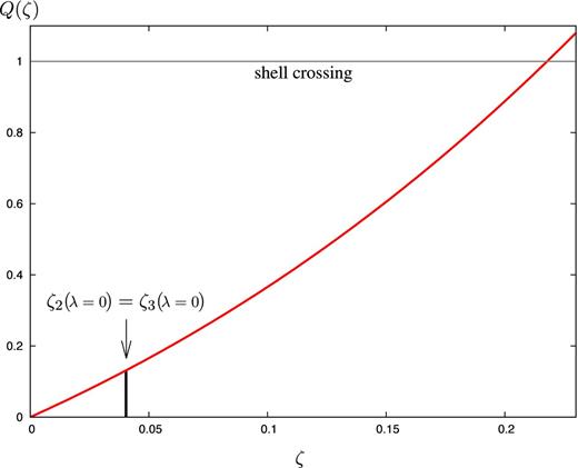
Lower bound on the norm of |J − 1| ≤ Q(ζ) = 6ζ3 + 6ζ2 + 3ζ, see equation (49). The vertical thick line at roughly ζ = 0.040 44 indicates the largest possible value of the smallest positive root ζ2(T(λ = 0)) of the polynomial |$p_\lambda (\mathfrak {a},\zeta )$| for which analyticity is guaranteed. Since ζ2(T(λ)) is a decreasing function of λ (see equation 52), it follows that |J − 1| < 0.132 for any value of Λ > 0, which is well below the value unity where shell-crossing might occur (the dotted line).
Analyticity in the linear growth function D
We have shown in Section 5 that the Lagrangian map |$\boldsymbol {x}(\boldsymbol {q},a)$| is an analytic function of a, near a = 0. The composition |$\boldsymbol {x}(\boldsymbol {q},a(D))$| of the Lagrangian map with the inverse linear growth function is also analytic in D. (This follows basically from the observation that analytic functions are complex-differentiable functions and the use of the chain rule.) We remark that this argument is not valid when the cosmic time is chosen as time variable, instead of D, as the relation between a and t is not analytic near the origin.
Can we obtain simple recursion relations for the D-Taylor coefficients of the displacement |$\boldsymbol {\xi }$|, as we have done in Section 4? Recursion relations, yes, but simple, no. Indeed, from equations (14) and (15), we can derive a set of Lagrangian Euler–Poisson equations in the time variable D. However the D-dependence is then essentially not polynomial, but will involve the full inverse linear growth function a(D), whose Taylor expansion has an infinite number of terms. As a consequence, the recursion relations will be very involved. If one really wants to reexpress the displacement as a power series in D, it is much simpler to just substitute the Taylor series for a(D), obtained by inversion of the Taylor series of D(a) into the expansion (16) in powers of a. Note that, with the latter strategy, there is no need to solve a succession of time differential equations for the nth order growth function (usually denoted with E, F, …), because the actual expansion parameter is precisely the cosmic scale factor, used as a time variable.
Effect on analyticity of the inclusion in the Friedmann equation of curvature and radiation terms
All this is not surprising: Actually, the curvature term in the Friedmann equation involves the inverse second power of the cosmic scale factor, which for a → 0 is subdominant with respect to the matter term a−3 and can thus not bring about much change. Very different would be the inclusion in the background of radiation effects, stemming from a blackbody distribution of photons. This adds a term in the Friedmann equation, proportional to the inverse fourth power of the scale factor, which drastically changes everything: slaving is lost, analyticity around a = 0 is lost, etc. The current favoured ΛCDM model has a background radiation density well below the matter density at decoupling and can actually be discarded after decoupling. When relating our results to numerical results or observations, it may be more convenient to use the cosmic time t rather than the a-time. Of course, when performing that change of variable, the radiation term in the Friedmann equation does not need to be omitted.
CONCLUDING REMARKS
In a Eulerian framework, space and time are intertwined by Galilean transformations (in the Newtonian approximation). It follows that, with the limited spatial smoothness assumed in the present work – roughly, that the initial density fluctuations are slightly better than continuous in the spatial variables – one cannot obtain better than a corresponding limited temporal smoothness. In a Lagrangian framework, as we have seen, the situation is drastically different: provided we use an appropriate time variable, such as the cosmic scale factor a or the linear growth function D. Obtaining analyticity in time of the Lagrangian trajectories requires then only a limited initial spatial smoothness.
Even more surprising is that this analyticity is around the point a = 0, which seems to extend this utterly smooth birth of our structured Universe to the very origin of time, well before decoupling of matter from photons. Of course, this is just a property of the mathematical model used here to describe structure formation, namely the Euler–Poisson equations in a ΛCDM Universe. The interesting feature is that this model allows us to have a well-posed problem, devoid of catastrophic behaviour near decoupling, provided we use the slaving conditions (10) at a = 0. These slaving conditions resemble those used to start N-body simulations at early times, (i) small density fluctuations, and (ii) an initial curl-free peculiar velocity field, related to the gravitational potential as in the Zel'dovich approximation. That these slaving conditions can be extended all the way to a = 0 means, from the point of view of boundary layer analysis (Cole 1968), that the matter-dominated era constitutes an outer solution for which, to leading order, the boundary matching to the inner solution (describing the primordial era) can be replaced by just an initial condition. This is true as long as, in the Friedmann equation for the background evolution in the matter-dominated era, we include only a matter term, a cosmological term and a possible curvature term, but no radiation term.
We remind the reader that our way of proving analyticity in the a-time is fully constructive. It rests indeed on a set of novel all-order recursion relations (26) for the time Taylor coefficients of the displacement of (fluid) particles. Not only are these relations fully explicit, but they have a very specific mathematical structure, allowing us to obtain bounds for all the Taylor coefficients and thus to establish analyticity by elementary means.
We now briefly indicate some of the possible future developments exploiting the analyticity result and the recursion relations. We shall mention two interlinked topics. One is about numerical integration of the Euler–Poisson equations by a multistep technique and the other one about cosmological reconstruction.
The Taylor method as described in Sections 4 and 5 allows us to determine the solution of the Euler–Poisson equations for any time 0 < a < R(0), where R(0) is the radius of convergence of the Taylor series around a = 0. (Here, it is best not to work with the rescaled time |$\mathfrak {a}$|.) A procedure, inspired from the Weierstrass analytic continuation technique for analytic functions, may allow us to obtain the solution beyond the time R(0). For this, we select a sequence of times 0 < a1 < a2 < a3 < … in such a way that an+1 is within the disc of convergence of the time Taylor series around the time an, that is such that |an+1 − an| < R(an), where R(a) is the radius of convergence of the Taylor expansion of the solution around time a. What we here call the solution is not just the Lagrangian map, but includes also the density which is controlled by the inverse of the Jacobian. Indeed, if the Jacobian vanishes, shell-crossing takes place and the Lagrangian map ceases to be invertible. Invertibility is essential, because at the end of each step, we must revert to an Eulerian description to be able to make a fresh start. Methods combining a Lagrangian step with a reversion to Eulerian coordinates are called semi-Lagrangian. A detailed description of a semi-Lagrangian method, called the Cauchy–Lagrangian method, which makes use of Cauchy's Lagrangian formulation of the ideal fluid dynamics can be found in Podvigina et al. (2015).
When dealing with the cosmological Euler–Poisson equations, the method of Podvigina et al. (2015) must be suitably adapted. One of the new difficulties stem from the non-autonomous character of our Euler–Poisson equations: the time appears explicitly in the equation. As a consequence, the Euler–Poisson equations are not invariant under a-time translations, but this problem can be circumvented.
In so far as the regime described by the Euler–Poisson equations does not include multi-streaming, a Cauchy–Lagrangian numerical method will not be able to address the same questions as N-body simulation techniques. There is however one important problem for which it appears well suited, namely the reconstruction of the dynamical history of the Universe from present-epoch galactic surveys (Frisch et al. 2002). It has been shown by Brenier et al. (2003) that the solution to the Euler–Poisson equations is uniquely determined by two boundary conditions, the slaving conditions (10) at the initial time and the density of matter at the current epoch. The latter is obtained from large galactic surveys. Euler–Poisson reconstruction is an extension of the variational N-body reconstruction, introduced by Peebles (1989) for handling galaxy data on relatively small scales, such as that of the Local Group. Euler–Poisson reconstruction, which is meant for significantly larger scales where a continuum description is applicable and where multistreaming can be ignored, does not suffer from the non-uniqueness problem of the variational N-body reconstruction. So far, Euler–Poisson reconstruction has not used the full solutions of the Euler–Poisson equations but just low-order Lagrangian perturbation approximations, such as the Zel'dovich approximation or the next order, denoted by 2LPT. Within such approximate frameworks, reconstruction becomes a Monge optimal transport problem (Frisch et al. 2002) with quadratic cost, which, after discretization, can be solved by very efficient assignment algorithms such as the auction method of Bertsekas (1992). Alternatively, one can use Brenier's theorem (Brenier 1987) and solve an equivalent 3D Monge–Ampère equation non-linear PDE by iterative techniques (Zheligovsky, Podvigina & Frisch 2010). Reconstruction by such methods is known as Monge–Ampère–Kantorovich (MAK). We propose to use the MAK reconstruction as a starting point of full Euler–Poisson reconstruction, applying an iterative Newton-type method in which at each stage a Euler–Poisson initial value problem is solved by a Cauchy–Lagrangian method.
Finally, we remind the reader that our proofs were given entirely within a Newtonian framework. In that framework, the time-analyticity results revealed a strong asymmetry between space and time in Lagrangian coordinates. The reason for that strong asymmetry is the ‘missing’ convective term in the Newtonian fluid equations, when formulated in Lagrangian coordinates. (In the notation of our Eulerian approach in Section 2, the convective term is |$\boldsymbol {v}\cdot \!{\nabla }_{\boldsymbol{x}}\boldsymbol {v}$|.) An interesting question is whether our time-analyticity results could be generalized to a Lagrangian coordinates formulation of a curl-free dust fluid in General Relativity. It is well known that the so-called synchronous-comoving coordinate system corresponds to a relativistic Lagrangian frame of reference, and, similar to the Lagrangian coordinates approach in the Newtonian framework, there is indeed no convective term in the relativistic equations of motion (in the so-called ADM approach; see e.g. Matarrese & Terranova 1996). These relativistic fluid equations are however decorated with Ricci tensors that involve (single and double) spatial gradients acting on the metric (and on its inverse), and this could well imply a limited temporal smoothness for limited spatial smoothness. Besides that unsolved problem, to obtain a time-analyticity result in General Relativity along lines similar to those of the present paper, it seems necessary to first obtain explicit all-order recursion relations. A possible starting point for such investigations could be the Lagrangian equations recently obtained by Alles et al. (2015).
We thank T. Buchert, A. Sobolevskiĭ, A. Wiegand and V. Zheligovsky for useful discussions and/or comments on the manuscript. UF and BV acknowledge the support of the Fédération Wolfgang Döblin (CNRS, Nice). CR acknowledges the support of the individual fellowship RA 2523/1-1 from the German research organization (DFG).
REFERENCES
