Revisiting the non-thermal radiation from the Crab nebula: requiring two distinct electron components

Zhu, Bo-Tao; Fang, Jun; Zhang, Li

doi:10.1093/mnras/stv1140

Abstract

We revisit the non-thermal radiation from the Crab nebula in the framework of a one-dimensional time-dependent model. In this model, two electron components are considered: a low-energy electron component, which has a power-law form, and a high-energy electron component, which has a power-law form or a relativistic Maxwellian plus a high-energy power-law tail. After fitting the observed multiband data of the Crab nebula using the Levenberg–Marquardt method of the χ²-minimization procedure, we show the following. (i) Electron injection with a relativistic Maxwellian plus a power-law tail (i.e. one electron population) cannot account for the observed multiband emission of the Crab nebula. (ii) Two distinct electron populations are required, although their origins are still under debate, and moreover there would be a low-energy electron component having a power-law form with a slope of ∼1.6 for the Crab nebula and Crab-like pulsar wind nebulae.

acceleration of particles, radiation mechanisms: non-thermal, ISM: individual objects: Crab Nebula, ISM: supernova remnants, gamma-rays: ISM

1 INTRODUCTION

The Crab nebula is powered by its pulsar PSR J0534+2200 and has been detected from radio to very high energy γ-rays. Without considering the Crab nebula's flares, the observed energy spectral distribution (SED) of non-thermal photons shows a two-peak shape. Theoretically, the first peak can be explained by synchrotron radiation of high-energy electrons, and the second peak by inverse Compton scattering of the lower energy seed photons by these electrons. These seed photons include the microwave background photons, the far-infrared (FIR), the starlight and the electron–synchrotron photons themselves (e.g. Atoyan & Aharonian 1996; Venter & de Jager 2007; Zhang, Chen & Fang 2008; Torres et al. 2014). Moreover, in modelling the SED of a pulsar wind nebula (PWN), a key quantity is the energy spectrum of the high-energy electrons, but the origin of these electrons is still under debate.

The electron's energy spectrum is generally assumed to be a power law, or a broken power law, or a relativistic Maxwellian plus a high-energy power-law tail. Generally, a single power-law electron spectrum cannot reproduce the multiband observational results of the Crab nebula but a broken power-law electron spectrum can (e.g. Atoyan & Aharonian 1996; Aharonian, Atoyan & Kifune 1997; Zhang et al. 2008; Torres et al. 2014). Atoyan & Aharonian (1996) explained the possible origin of the broken power-law electron spectrum as follows. There are two populations of relativistic electrons inside the PWN. The electrons created inside the light cylinder of the pulsar form the low-energy part with an index of ∼1.5 at energy E ≤ E_b (where E_b is the broken energy). Because these electrons mainly contribute to radio photons by synchrotron radiation, they are called radio electrons. At E > E_b, the electrons produced beyond the light cylinder at the shock radius by the Fermi-type process (Achterberg et al. 2001) form the high-energy part with an index ≥2 (called the wind electron component). For the third possible electron spectrum, because of a pulsar wind (magnetic flux plus high-energy particles) that flows relativistically into the non-relativistic ejecta of the ambient supernova remnant (SNR), the particle spectrum downstream of a relativistic shock is a relativistic Maxwellian and a high-energy power-law tail with an index of −2.4 ± 0.1 (Spitkovsky 2008). Note that Sironi & Spitkovsky (2011) have recently studied the process of driven magnetic reconnection at the termination shock of relativistic striped flows through two-dimensional (2D) and three-dimensional (3D) particle-in-cell simulations. They have shown that the reconnection electric field at the X-points can accelerate the particles. They have found that whether the shape of the post-shock spectrum has a power-law form with an index α depends primarily on the ratio λ/(r_Lσ), where λ is the stripe wavelength, r_L is the relativistic Larmor radius in the wind and σ is the wind magnetization. Sironi & Spitkovsky (2011) have shown that the post-shock spectrum is a Maxwellian-like spectrum for small values λ/(r_Lσ) (≲ a few tens), but approaches a broad power-law tail with slope α ∼ 1.5 for very large values of λ/(r_Lσ) (≳ a few hundred); see also Sironi & Spitkovsky (2012). When applying this to the Crab pulsar, however, they found that a Maxwellian-like spectrum would be predicted because λ/(r_Lσ) ≲ 0.01 (Sironi & Spitkovsky 2011, 2012). If this is true, then the spectrum cannot account for observed radio emission from the Crab pulsar. Therefore, there should be another origin for the low-energy electron component and two distinct electron populations should be present in PWNe.

In the one-dimensional (1D) model of the dynamical and radiative evolution of a pulsar wind nebula in a non-radiative SNR, Gelfand, Slane & Zhang (2009) investigated the radiative properties during different phases of the PWN evolution, assuming a single power-law injection spectrum for the electrons/positrons. Fang & Zhang (2010) discussed the radiative properties during a different phase of the PWN by assuming the relativistic Maxwellian and a high-energy power-law tail injection spectrum for the electrons/positrons. They applied the model to three composite SNRs: G0.9+0.1, MSH 15–52 and G338.3–0.0. The model also applied to HESS J1640–465 (Slane et al. 2010) and MSH 11–62 (Slane et al. 2012). Note that one electron population is required in this case.

In this paper, we study the radiative properties of the Crab nebula in the model given by Gelfand et al. (2009). Because the exact nature of two electron components is still unknown (e.g. Vorster et al. 2013), we consider two possible forms of injected electron spectra. The first form is a broken power law and the other is the sum of a power law at low energy and a relativistic Maxwellian plus a high-energy power-law tail. Then, we fit the observed multiband spectrum of the Crab pulsar using the Levenberg–Marquardt (LM) method of the χ²-minimization fitting procedure, instead of eyeball fitting. We have found that the electron spectrum with a relativistic Maxwellian plus a high-energy power-law tail cannot absolutely explain the observed data of the Crab nebula, if there is no low-energy component of the injection spectrum.

The structure of this paper is as follows. In Section 2, we briefly review the model. In Section 3, we apply the model to the Crab PWN, and research its multiband non-thermal emission. In Section 4, we give a discussion and our conclusions.

2 ELECTRON INJECTION AND A PWN EVOLUTION

2.1 Injected electron spectra

As mentioned in Section 1, there are two different populations of electrons in the Crab nebula, and we consider two possible forms of the injected electron spectra in this section.

The first form is the broken power law, which has been widely used in the literature (e.g. Venter & de Jager 2007; Zhang et al. 2008; Tanaka & Takahara 2010; Vorster et al. 2013; Torres et al. 2014). This can be expressed as

\begin{equation} Q_{\rm I}(E,t) = Q_0(t)\left\lbrace \begin{array}{ll}\displaystyle \left(\frac{E}{E_{\rm b}}\right)^{-\alpha _1}&\quad {\rm for}\ E\le E_{\rm b},\\ \displaystyle \left(\frac{E}{E_{\rm b}}\right)^{-\alpha _2}&\quad {\rm for}\ E_{\rm b}\le E <E_{\rm max}, \end{array} \right. \end{equation}

(1)

where |$Q_0(t)(E/E_{\rm b})^{-\alpha _1}$| represents the low-energy component of the injection spectrum with an index α₁ ∼ 1.5, |$Q_0(t)(E/E_{\rm b})^{-\alpha _2}$| is the high-energy component of the injection spectrum with an index α₂ > 2.0 and E_b is the break energy, which can be roughly estimated by equating the electron's synchrotron cooling time to the lifetime of the Crab pulsar.

In equation (1), E_max is the maximum energy of the electrons and can be estimated as follows. If the spin-down power of the pulsar is assumed to be only distributed between electrons [|$\dot{E}_{\rm e}(t) = \eta _{\rm e} L(t)$|] and magnetic fields [|$\dot{E}_{B}= \eta _{B}L(t)]$|⁠, where η_e + η_B = 1 (Gelfand et al. 2009), then in order to confine the accelerated particles within the PWN, it is necessary for the radius r_pwn of the PWN to be larger than the Larmor radius r_L = E_max/eB_pwn of the electrons inside the PWN (i.e. r_L = ϵr_pwn with ϵ < 1). This is given by

\begin{equation} E_{\rm max}=\epsilon \kappa e\sqrt{\frac{\eta _{B}L(t)}{c}}\approx 3\epsilon e\sqrt{\frac{\eta _{B}L(t)}{c}}\;, \end{equation}

(2)

where e is the electron charge. A compression factor κ ≈ 3 (Kennel & Coroniti 1984; Tanaka & Takahara 2010; Martin, Torres & Rea 2012), the magnetic field strength of the PWN, |$B_{\rm pwn}\approx \kappa \sqrt{\eta _{B}L(t)/c}/r_{\rm pwn}$|⁠, has been used in equation (2). Moreover, Q₀(t) is a time-dependent parameter, which relates to the spin-down power L(t) of the pulsar, and can be determined by

\begin{equation} (1-\eta _B)L(t) = \int _{0}^{E_{\rm max}} Q(E, t) E \,{\rm d}E, \end{equation}

(3)

that is,

\begin{eqnarray} Q_0(t) = \left\lbrace \begin{array}{ll}\displaystyle \frac{(1-\eta _{B})L(t)}{{E_{\rm b}}^2}\frac{(2-\alpha _1)(2-\alpha _2)}{\alpha _1-\alpha _2} &\quad \alpha _2> 2,\\ \displaystyle \frac{(1-\eta _{B})L(t)}{{E_{\rm b}}^2}\left[\frac{1}{2-\alpha _1} + \log \left({\frac{E_{\rm max}}{E_{\rm b}}}\right)\right] &\quad \alpha _2 =2. \end{array} \right.\nonumber\\ \end{eqnarray}

(4)

For the second form, two electron components are also assumed: one is described by |$Q_1(E,t) = Q^{\prime }_0(t)(E/E_{\rm b_1})^{-\alpha _1^{\prime }}$| for |$E\le E_{\rm b}^{\prime } <E_{\rm b_1}$|⁠, and the other has the form of a relativistic Maxwellian and a high-energy power-law tail. For the latter, we use the expression given by Fang & Zhang (2010). Therefore, the second form of the injection spectrum can be written as

\begin{eqnarray*} Q_{\rm II}(E, t)= Q^{\prime }_0(t) \end{eqnarray*}

\begin{equation} \left\lbrace \begin{array}{ll}\displaystyle \left(\frac{E}{E_{\rm b_1}}\right)^{-\alpha _1^{\prime }} + g\left(\frac{E}{E_{\rm b_1}}\right) &\quad E\le E_{\rm b}^{\prime } ,\\ \displaystyle g\left(\frac{E}{E_{\rm b_1}}\right) &\quad E_{\rm b}^{\prime } <E \le E_{\rm min},\\ \displaystyle \left[g\left(\frac{E}{E_{\rm b_1}}\right) + f\left(\frac{E}{E_{\rm b_1}}\right)^{-\alpha _2^{\prime }}\right] &\quad E_{\rm min}<E \le E_{\rm max}, \end{array} \right. \end{equation}

(5)

where |$g(E/E_{\rm b_1})= (E/E_{\rm b_1})\exp (-E/E_{\rm b_1})$|⁠, |$E_{\rm b_1}=0.26 (\gamma _{\rm st}/10^6)$| TeV, γ_st is the Lorentz factor of the upstream pulsar wind of the termination shock (Spitkovsky 2008), |$E_{\rm min}\approx 7 E_{\rm b_1}$|⁠, |$\alpha _2^{\prime }=2.4\pm 0.1$| and the factor f is given by |$f=(E_{\rm min}/E_{\rm b_1})^{\alpha _2^{\prime }+1} \exp (-E_{\rm min}/E_{\rm b_1})\approx 0.68$|⁠. In equation (5), |$Q^{\prime }_0(t)$| is also the time-dependent parameter. Using equation (3), we have

\begin{eqnarray} Q^{\prime }_0(t) &=& \left[{(1-\eta ^{\prime }_{B})L(t)}\right]\Bigg [E^2_{\rm b_1}\Bigg \lbrace \left(\frac{E_{\rm b}^{\prime }}{E_{{\rm b}_1}}\right)^{\beta _1} + 2\nonumber \\ &&+\, \frac{f}{\beta } \left[ \left( \frac{E_{\rm max}}{E_{\rm b_1}} \right)^{\beta } - \left( \frac{E_{\rm min}}{E_{\rm b_1}} \right)^{\beta }\right]\Bigg \rbrace \Bigg ]^{-1}, \end{eqnarray}

(6)

where |$\beta _1=2-\alpha _1^{\prime }$| and |$\beta =2-\alpha _2^{\prime }$|⁠. Note that if we consider the injection with the Maxwellian plus a higher-energy power law alone, then the injection spectrum can be expressed as

\begin{eqnarray*} Q_{\rm III}(E, t) = Q^{\prime \prime }_0(t) \end{eqnarray*}

\begin{equation} \left\lbrace \begin{array}{ll}\displaystyle g\left(\frac{E}{E^{\prime }_{\rm b_1}}\right) &\quad E \le E^{\prime }_{\rm min},\\ \displaystyle \left[g\left(\frac{E}{E^{\prime }_{\rm b_1}}\right) + f\left(\frac{E}{E^{\prime }_{\rm b_1}}\right)^{-\alpha ^{\prime \prime }}\right] &\quad E^{\prime }_{\rm min}<E \le E_{\rm max}, \end{array} \right. \end{equation}

(7)

and

\begin{eqnarray} Q^{\prime \prime }_0(t) &=& \left[{(1-\eta ^{\prime \prime }_{B})L(t)}\right]\Bigg [E^{\prime 2}_{\rm b_1}\Bigg \lbrace 2 + \frac{f}{\beta ^{\prime }} \Bigg [ \left( \frac{E^{\prime }_{\rm max}}{E^{\prime }_{\rm b_1}} \right)^{\beta ^{\prime }} \nonumber \\ &&\qquad\qquad\qquad\,\,- \left( \frac{E_{\rm min}}{E^{\prime }_{\rm b_1}}\right)^{\beta ^{\prime }}\Bigg ]\Bigg \rbrace \Bigg ]^{-1}, \end{eqnarray}

(8)

with β^′ = 2 − α^′^′.

Finally, the evolution of the spin-down power L(t) with time is needed. For a given pulsar with a period P, a period derivative |$\dot{P}$| and a braking index n, the relation between the initial spin-down power L₀ and the spin-down power L(t) at time t is given by (Gaensler & Slane 2006)

\begin{equation} {L}(t)={L}_0\left(1+\frac{t}{\tau _0}\right)^{-(n+1)/(n-1)}. \end{equation}

(9)

Here, τ₀ is the initial spin-down time-scale of the pulsar and

\begin{equation} \tau _0=\frac{P_0}{(n-1)\dot{P_0}}=\frac{2\tau _{\rm c}}{n-1}-t_{\rm age}, \end{equation}

(10)

where |$\tau _{\rm c} =P/2\dot{P}$| is the characteristic age of the pulsar and t_age is the age of the Crab nebula.

2.2 Dynamical and radiative evolution of a PWN

As mentioned in Section 1, Gelfand et al. (2009) presented a PWN model that can self-consistently describe the dynamical and radiative evolution of a PWN in a non-radiative SNR (also see Fang & Zhang 2010). In this model, the large-scale evolution of a composite SNR depends on the mechanical energy E_sn of the explosion, the density ρ_ISM of the ambient medium, the mass M_ej of the supernova ejecta and the spin-down power L(t) of the pulsar. Additional parameters of considerable importance are the braking index n and initial spin-down time-scale τ₀ of the pulsar, along with the fraction η_B of the spin-down power that appears as magnetic flux. However, once the injected electron rate Q_i(E, t) (i = I, II, III) is given, the evolution of the electron distribution N(E, t) in the emission region is calculated by using the following equation:

\begin{equation} \frac{{\mathrm{\partial} } N(E,t)}{{\mathrm{\partial} } t}= \frac{{\mathrm{\partial} } }{{\mathrm{\partial} } E} \left[ \dot{E} N(E,t) \right] + \frac{N(E,t)}{\tau (E,t)} + Q_i(E,t). \end{equation}

(11)

Here, the isotropic distribution of the electrons in the PWN is assumed, |$\dot{E}$| is the energy-loss rate of the particles with energy E, which includes the contributions of synchrotron radiation, inverse Compton scattering and adiabatic losses, τ(E, t) is the escape time (the details of their processes are given in Zhang et al. 2008). Then, the multiwavelength non-thermal photon spectrum can be calculated (the details of their processes are given in Zhang et al. 2008) and the properties of the radiative evolution for a given PWN can be determined. In this paper, we consider the non-thermal photon emission through synchrotron radiation and inverse Compton scattering of the soft seed photons, where the four different seed photon fields involved are: (i) the synchrotron radiation photon; (ii) the 2.7-K CMB radiation with an energy density U_CMB = 0.25 eV cm⁻³; (iii) the excess FIR radiation with an energy density U_FIR = 0.5 eV cm⁻³ and a temperature 70 K; (iv) the starlight with an energy density U_star = 1.0 eV cm⁻³ and a temperature 5000 K.

In this model, there are over ten parameters. In order to fit the observed multiwavelength data for a given PWN, we divided the model parameters into two parts: adopted and fitted parameters. The adopted parameters include observed quantities (e.g. period P, its derivative |$\dot{P}$|⁠, the distance d, the braking index n, pulsar age t_age and pulsar velocity v_spr) and derived or commonly assumed quantities (e.g. the initial spin-down power L₀, initial spin-down age τ₀, the ISM density n_H, E_sn and M_ej). The rest of the parameters are fitted parameters. We use the LM algorithm given by Press et al. (1992) to fit the observed multiwavelength data for a given PWN.

3 APPLICATION TO THE CRAB NEBULA

The Crab nebula lies at a distance of 2 kpc (e.g. Manchester et al. 2005). Its pulsar has a rotational period P = 33.4 ms, a period derivative |$\dot{P}=4.23\times 10^{-13}$| s s⁻¹, L(t) = 4.53 × 10³⁸ erg s⁻¹ (e.g. Taylor, Manchester & Lyne 1993), a braking index n = 2.509 (e.g. Lyne, Pritchard & Graham-Smith 1993) and a pulsar velocity of 120 km s⁻¹ (e.g. Kaplan et al. 2008). Following Bucciantini, Arons & Amato (2011), we assume that E_sn = 1 × 10⁵¹ erg, M_ej = 9.5 M_⊙ and n_H = 0.1 cm⁻³. Observationally, the Crab nebula has been detected in radio (Baldwin 1971; Macías-Pérez et al. 2010), IR (Ney & Stein 1968; Grasdalen 1979; Temim et al. 2006), optical (Veron-Cetty & Woltjer 1993), X-ray soft-γ ray (Hennessy et al. 1992; Kuiper et al. 2001) and γ-ray band (Aharonian et al. 2004, 2006; Albert et al. 2008; Abdo et al. 2010).

For a given injection spectrum, the key parameter that has an important influence on the dynamical properties is the magnetic fraction η_B. In this paper, we consider three types of electron injection spectra. The adopted parameters in our calculations are listed in Table 1. There is a small difference in their magnetic fractions for the three types of electron injection spectra, so the dynamical properties of the Crab nebula are almost the same for the three types of the electron injections. For example, when using two different injection spectra to fit the observed multiband data process, on the one hand, we find the R_pwn ≈ 1.98 pc for the first form of the electron injection spectrum (equation 1) and R_pwn ≈ 2.02 pc for the second form of the electron's injection spectrum (equation 5). On the other hand, the current magnetic field strength of the Crab nebula is B = 122 μG for the first form of the electron injection spectrum and B = 130 μG for the second form of the electron injection spectrum, which are constrained to be between 100 and 200 μG (e.g. Abdo et al. 2010). In fact, the dynamical properties of the PWN during the evolution are similar to those in Gelfand et al. (2009).

Table 1.

Open in new tab

Input and fitted parameters for the Crab nebula.

	Symbol	Value
Adopted parameter
Ejected mass (M_⊙)	M_ej	9.5
SN explosion energy (10⁵¹erg)	E_sn	1.0
Hydrogen density (cm³)	n_H	0.1
Period (ms)	P	33.4
Period derivative (⁠\|$\rm s \cdot \rm s^{-1}$\|⁠)	\|$\dot{{\it P}}$\|	4.23 × 10⁻¹³
Initial spin-down luminosity	L₀	0.31
(10⁴⁰ erg s⁻¹)
Initial spin-down age (yr)	τ₀	730
Braking index	n	2.509
Pulsar velocity (km s⁻¹)	\|${v}^{}_{\rm psr}$\|	120
Age (yr)	t_age	940
Distance (kpc)	d	2.0
Injection spectrum: equation (1)
Fitted parameter \|$\boldsymbol {\chi ^2}$\| = 1.6
Magnetic fraction	η_B	0.046 ± 0.002
Shock radius fraction	ϵ	0.159 ± 0.009
Low-energy electron index	α₁	1.607 ± 0.006
Wind electron index	α₂	2.413 ± 0.005
Break energy (10⁵ MeV)	E_b	6.2 ± 0.4
Injection spectrum: equation (5)
Fitted parameter \|$\boldsymbol {\chi ^2}$\| = 2.1
Magnetic fraction	\|$\eta ^{\prime }_B$\|	0.055 ± 0.002
Shock radius fraction	ϵ^′	0.142 ± 0.004
Low-energy electron index	\|${\alpha }_{1}^{\prime }$\|	1.678 ± 0.003
Wind electron index	\|${\alpha }_{2}^{\prime }$\|	2.378 ± 0.005
Low-energy break energy	\|$E_{\rm b}^{\prime }$\|	4.60 ± 0.03
(10⁵ MeV)
Break energy (10⁵ MeV)	\|$E_{\rm b_1}$\|	7.6 ± 0.3
Injection spectrum: equation (7)
Fitted parameter \|$\boldsymbol {\chi ^2}$\| = 50.2
Magnetic fraction	\|$\eta ^{\prime \prime }_{B}$\|	0.062 ± 0.001
Shock radius fraction	ϵ^′^′	0.147 ± 0.001
Wind electron index	α^′^′	2.425 ± 0.006
Break energy (10⁵ MeV)	\|$E_{\rm b_1}^{\prime }$\|	5.61 ± 0.02

	Symbol	Value
Adopted parameter
Ejected mass (M_⊙)	M_ej	9.5
SN explosion energy (10⁵¹erg)	E_sn	1.0
Hydrogen density (cm³)	n_H	0.1
Period (ms)	P	33.4
Period derivative (⁠\|$\rm s \cdot \rm s^{-1}$\|⁠)	\|$\dot{{\it P}}$\|	4.23 × 10⁻¹³
Initial spin-down luminosity	L₀	0.31
(10⁴⁰ erg s⁻¹)
Initial spin-down age (yr)	τ₀	730
Braking index	n	2.509
Pulsar velocity (km s⁻¹)	\|${v}^{}_{\rm psr}$\|	120
Age (yr)	t_age	940
Distance (kpc)	d	2.0
Injection spectrum: equation (1)
Fitted parameter \|$\boldsymbol {\chi ^2}$\| = 1.6
Magnetic fraction	η_B	0.046 ± 0.002
Shock radius fraction	ϵ	0.159 ± 0.009
Low-energy electron index	α₁	1.607 ± 0.006
Wind electron index	α₂	2.413 ± 0.005
Break energy (10⁵ MeV)	E_b	6.2 ± 0.4
Injection spectrum: equation (5)
Fitted parameter \|$\boldsymbol {\chi ^2}$\| = 2.1
Magnetic fraction	\|$\eta ^{\prime }_B$\|	0.055 ± 0.002
Shock radius fraction	ϵ^′	0.142 ± 0.004
Low-energy electron index	\|${\alpha }_{1}^{\prime }$\|	1.678 ± 0.003
Wind electron index	\|${\alpha }_{2}^{\prime }$\|	2.378 ± 0.005
Low-energy break energy	\|$E_{\rm b}^{\prime }$\|	4.60 ± 0.03
(10⁵ MeV)
Break energy (10⁵ MeV)	\|$E_{\rm b_1}$\|	7.6 ± 0.3
Injection spectrum: equation (7)
Fitted parameter \|$\boldsymbol {\chi ^2}$\| = 50.2
Magnetic fraction	\|$\eta ^{\prime \prime }_{B}$\|	0.062 ± 0.001
Shock radius fraction	ϵ^′^′	0.147 ± 0.001
Wind electron index	α^′^′	2.425 ± 0.006
Break energy (10⁵ MeV)	\|$E_{\rm b_1}^{\prime }$\|	5.61 ± 0.02

Table 1.

Open in new tab

Input and fitted parameters for the Crab nebula.

	Symbol	Value
Adopted parameter
Ejected mass (M_⊙)	M_ej	9.5
SN explosion energy (10⁵¹erg)	E_sn	1.0
Hydrogen density (cm³)	n_H	0.1
Period (ms)	P	33.4
Period derivative (⁠\|$\rm s \cdot \rm s^{-1}$\|⁠)	\|$\dot{{\it P}}$\|	4.23 × 10⁻¹³
Initial spin-down luminosity	L₀	0.31
(10⁴⁰ erg s⁻¹)
Initial spin-down age (yr)	τ₀	730
Braking index	n	2.509
Pulsar velocity (km s⁻¹)	\|${v}^{}_{\rm psr}$\|	120
Age (yr)	t_age	940
Distance (kpc)	d	2.0
Injection spectrum: equation (1)
Fitted parameter \|$\boldsymbol {\chi ^2}$\| = 1.6
Magnetic fraction	η_B	0.046 ± 0.002
Shock radius fraction	ϵ	0.159 ± 0.009
Low-energy electron index	α₁	1.607 ± 0.006
Wind electron index	α₂	2.413 ± 0.005
Break energy (10⁵ MeV)	E_b	6.2 ± 0.4
Injection spectrum: equation (5)
Fitted parameter \|$\boldsymbol {\chi ^2}$\| = 2.1
Magnetic fraction	\|$\eta ^{\prime }_B$\|	0.055 ± 0.002
Shock radius fraction	ϵ^′	0.142 ± 0.004
Low-energy electron index	\|${\alpha }_{1}^{\prime }$\|	1.678 ± 0.003
Wind electron index	\|${\alpha }_{2}^{\prime }$\|	2.378 ± 0.005
Low-energy break energy	\|$E_{\rm b}^{\prime }$\|	4.60 ± 0.03
(10⁵ MeV)
Break energy (10⁵ MeV)	\|$E_{\rm b_1}$\|	7.6 ± 0.3
Injection spectrum: equation (7)
Fitted parameter \|$\boldsymbol {\chi ^2}$\| = 50.2
Magnetic fraction	\|$\eta ^{\prime \prime }_{B}$\|	0.062 ± 0.001
Shock radius fraction	ϵ^′^′	0.147 ± 0.001
Wind electron index	α^′^′	2.425 ± 0.006
Break energy (10⁵ MeV)	\|$E_{\rm b_1}^{\prime }$\|	5.61 ± 0.02

	Symbol	Value
Adopted parameter
Ejected mass (M_⊙)	M_ej	9.5
SN explosion energy (10⁵¹erg)	E_sn	1.0
Hydrogen density (cm³)	n_H	0.1
Period (ms)	P	33.4
Period derivative (⁠\|$\rm s \cdot \rm s^{-1}$\|⁠)	\|$\dot{{\it P}}$\|	4.23 × 10⁻¹³
Initial spin-down luminosity	L₀	0.31
(10⁴⁰ erg s⁻¹)
Initial spin-down age (yr)	τ₀	730
Braking index	n	2.509
Pulsar velocity (km s⁻¹)	\|${v}^{}_{\rm psr}$\|	120
Age (yr)	t_age	940
Distance (kpc)	d	2.0
Injection spectrum: equation (1)
Fitted parameter \|$\boldsymbol {\chi ^2}$\| = 1.6
Magnetic fraction	η_B	0.046 ± 0.002
Shock radius fraction	ϵ	0.159 ± 0.009
Low-energy electron index	α₁	1.607 ± 0.006
Wind electron index	α₂	2.413 ± 0.005
Break energy (10⁵ MeV)	E_b	6.2 ± 0.4
Injection spectrum: equation (5)
Fitted parameter \|$\boldsymbol {\chi ^2}$\| = 2.1
Magnetic fraction	\|$\eta ^{\prime }_B$\|	0.055 ± 0.002
Shock radius fraction	ϵ^′	0.142 ± 0.004
Low-energy electron index	\|${\alpha }_{1}^{\prime }$\|	1.678 ± 0.003
Wind electron index	\|${\alpha }_{2}^{\prime }$\|	2.378 ± 0.005
Low-energy break energy	\|$E_{\rm b}^{\prime }$\|	4.60 ± 0.03
(10⁵ MeV)
Break energy (10⁵ MeV)	\|$E_{\rm b_1}$\|	7.6 ± 0.3
Injection spectrum: equation (7)
Fitted parameter \|$\boldsymbol {\chi ^2}$\| = 50.2
Magnetic fraction	\|$\eta ^{\prime \prime }_{B}$\|	0.062 ± 0.001
Shock radius fraction	ϵ^′^′	0.147 ± 0.001
Wind electron index	α^′^′	2.425 ± 0.006
Break energy (10⁵ MeV)	\|$E_{\rm b_1}^{\prime }$\|	5.61 ± 0.02

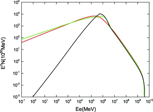
We now consider the electron spectra at the current time for the Crab nebula. In Fig. 1, we show the electron spectra of the Crab nebula at current time t_age = 940 yr for three types of electron injection given by equations (1), (5) and (7). The three types of electron spectra are the same power-law form with a slightly different spectral index at the high-energy end of E ≥ E_min ≈ 6 TeV (see Table 1). However, we have considered the escape effect of the electrons (see equation 11), and find that the escape effect is negligible for young PWNe such as the Crab nebula.

Figure 1.

Electron spectra of the Crab nebula at current time t_age = 940 yr for three types of electron injection. The red, green and black curves represent the electron spectra in which the injection spectra are given by equations (1), (5) and (7), respectively. Model parameters are listed in Table 1.

Open in new tab Download slide

Using the electron spectra of the Crab nebula at the current time, we can calculate the corresponding SEDs and compare them with the observed data. The non-thermal component consists of electron synchrotron radiation and inverse Compton scattering of the soft seed photons (for details, see Zhang et al. 2008). As mentioned above, for a given electron injection spectrum, model parameters are divided into adopted and fitted parameters, and then a model fit to the observed multiband data is made by using the LM method of the χ²-minimization procedure instead of eyeball fitting. In this process, data for the IR bump at ∼0.01 eV are excluded, because this emission is thought to be dominated by thermal dust emission by the PWN. In Fig. 2, we show the fitting result for the electron injection spectrum given by equation (1) (the values of the fitted parameters are listed in Table 1). It can be seen from the figure that the non-thermal photon emission below the energy E ≈ 200 MeV is dominated by the synchrotron radiation of the electrons; above E ≈ 200 MeV, the inverse Compton scattering process dominates the non-thermal photon emission. In Fig. 3, we show the fitting result for the case in which the electron injection spectrum is given by equation (5). The calculated result in this case can also fit the observed data well (the values of the fitted parameters are listed in Table 1).

Figure 2.

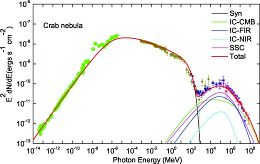
Fit of the Crab nebula SED calculated in the case of the electron injection spectrum with a broken power law to observed multiband data. The calculated SEDs of synchrotron emission (black line), inverse Compton scatterings with the synchrotron photons (magenta line), IR (blue line), CMB (green line), starlight (cyan line) and total emission (red line) are shown. The observed data are taken from Baldwin (1971) and Macías-Pérez et al. (2010) at radio band, from Ney & Stein (1968), Grasdalen (1979) and Temim et al. (2006) at IR band, from Veron-Cetty & Woltjer (1993) at optical band, from Hennessy et al. (1992) and Kuiper et al. (2001) at X-ray and soft-γ ray bands and from Aharonian et al. (2004, 2006), Albert et al. (2008) and Abdo et al. (2010) at γ-ray band. The adopted and fitted parameters are listed in Table 1.

Open in new tab Download slide

Figure 3.

Same as Fig. 2 but for the case in which the electron injection spectrum is given by equation (5). The adopted and fitted parameters are listed in Table 1.

Open in new tab Download slide

Finally, using the LM method of the χ²-minimization procedure, we fit the observed multiband data of the Crab nebula for the case in which the electron injection spectrum is given by equation (7) (i.e. the injection spectrum is a relativistic Maxwellian plus a high-energy power-law tail). We show the fitting result in Fig. 4 and the model parameters in Table 1. It is clear that in this case the lower-energy part of the observed data cannot be fitted and χ² ≈ 50 is obtained. Therefore, we can conclude that electron injection with a relativistic Maxwellian plus a power-law tail (i.e. one electron population) cannot explain the observed multiband emission of the Crab nebula.

Figure 4.

Same as Fig. 2 but for the case in which the electron injection spectrum is given by equation (7). The adopted and fitted parameters are listed in Table 1.

Open in new tab Download slide

4 SUMMARY AND DISCUSSION

In this paper, we have investigated multiband non-thermal emission properties of the Crab nebula in the PWN model given by Gelfand et al. (2009) with three types of injected electron forms. After fitting the observed multiband data of the Crab nebula by using the LM method of the χ²-minimization procedure, we have shown that a single electron component with a relativistic Maxwellian plus a power-law tail cannot account for the observed multiband data of the Crab nebula (see Fig. 4 and Table 1), and a low-energy electron component is required (i.e. two distinct electron components are needed). Although the cut-off energies of the component are different for the injection forms given by equations (1) and (5) (see Table 1), the component has a power-law form with the slope of ∼1.6.

Different injection forms have a little influence on the PWN dynamical properties. For example, our results show that the current magnetic field strength and the current radius of the Crab nebula are B ≈ 122 μG and R_pwn ≈ 1.98 pc for the first injection form given by equation (1), and B ≈ 130 μG and R_pwn ≈ 2.02 pc for the second injection form given by equation (5). These values are slightly larger than those given by Gelfand et al. (2009). The main reason for the differences is the different values of magnetic fraction η_B. In fact, Gelfand et al. (2009) gave η_B = 10⁻³ as an input parameter and did not fit the multiband data of the Crab nebula (they assumed a single power-law form for the electron injection). However, in our work, η_B is a fitted parameter, and η_B ∼ 0.05 and η_B ∼ 0.06 for the two injection forms, respectively (see Table 1).

As mentioned in Section 1, the origin of the low-energy electron component is still debatable. Currently, there are at least two possible origins. The first origin is that the electrons at the low-energy region are produced in the light cylinder of the pulsar (e.g. Atoyan & Aharonian 1996). The second origin is that these low-energy electrons are accelerated by relativistic magnetic reconnection in a PWN (e.g. Sironi & Spitkovsky 2011, 2012, 2014). However, for the Crab nebula, Sironi & Spitkovsky (2011) pointed out that a power-law form with a slope ∼1.5 for the low-energy electron component cannot be obtained unless the multiplicity in the pulsar wind is as large as 10⁸ along the equatorial plane, because λ/(r_Lσ) is proportional to the multiplicity. However, such high multiplicity is not predicted by available models.

We would like to thank the anonymous referee for instructive comments. This work is partially supported by the National Natural Science Foundation of China (NSFC 11433004, 11103016, 11173020), the Doctoral Fund of the Ministry of Education of China (RFDP 20115301110005), the Key Project of the Chinese Ministry of Education (212160), the Top Talents Programme of Yunnan Province, the Applied Basic Research Project of Yunnan Province (2011FB012) and the Light of the Western Talent Training Project (W8090303).

REFERENCES

Abdo

A. A.

et al.

ApJ

2010

708

1254

Month:	Total Views:
February 2017	1
March 2017	4
April 2017	6
July 2017	1
August 2017	1
September 2017	1
October 2017	11
November 2017	3
December 2017	2
January 2018	2
February 2018	1
March 2018	3
April 2018	3
May 2018	3
June 2018	6
July 2018	2
August 2018	12
September 2018	4
October 2018	11
November 2018	10
December 2018	6
January 2019	6
February 2019	8
March 2019	5
April 2019	11
May 2019	11
June 2019	6
July 2019	8
August 2019	3
September 2019	6
October 2019	5
November 2019	9
December 2019	11
January 2020	5
February 2020	4
March 2020	6
April 2020	5
May 2020	1
June 2020	4
July 2020	3

Article Contents

Revisiting the non-thermal radiation from the Crab nebula: requiring two distinct electron components Free

Abstract

1 INTRODUCTION

2 ELECTRON INJECTION AND A PWN EVOLUTION

2.1 Injected electron spectra

2.2 Dynamical and radiative evolution of a PWN

3 APPLICATION TO THE CRAB NEBULA

4 SUMMARY AND DISCUSSION

REFERENCES

Citations

Views

Altmetric

Email alerts

Astrophysics Data System

Citing articles via

Latest

Most Read

Most Cited

This Feature Is Available To Subscribers Only

Revisiting the non-thermal radiation from the Crab nebula: requiring two distinct electron components