Abstract
In this article, we discuss the magnetic field inertia that results in the so-called anomalous electromagnetic torque, making neutron stars precess. We focus particularly on the relative contribution of fields of different scales and show that small-scale fields may produce an anomalous torque comparable in magnitude with the one produced by dipolar field. Also, the internal toroidal field may play an important role. If the stellar magnetic field is not symmetric with respect to the dipolar moment axis, the pulsar inclination angle may oscillate with a typical amplitude of tens of degrees, due to precession. Such variations may, in principle, be observable.
1 INTRODUCTION
The electromagnetic torque acting on rotating neutron stars consists of two components. The first component is related to angular momentum transfer away from the star to infinity by both particles and electromagnetic radiation. The second component is the so-called anomalous torque. It is caused by inertia of the near-zone electromagnetic field. The first component is determined almost exclusively by the magnetic dipole moment of the star (see, however, Barsukov, Goglichidze & Tsygan 2013). As for the anomalous torque, its amount and direction essentially depend on the structure of the internal and external field, as will be seen.
To date, much observational and theoretical evidence has been accumulated suggesting that the magnetic field near the surface of a neutron star differs substantially from the dipolar field, the value of which is usually determined by pulsar spin-down, assuming that pulsars lose their rotational energy due to magnetic dipole radiation. This can be up to 1–2 orders of magnitude stronger and apparently contains an essential small-scale component. Some pulsars have features in their X-ray spectra: for instance, the millisecond pulsar B1821+24 has a feature slightly above 3 keV (Becker et al. 2003). This feature is interpreted as an electron cyclotron line formed at magnetic field ≈3 × 10¹¹ G, while the field value determined by the spin-down rate equals 4.6 × 10⁹ G. X-ray pulsar 1E 1207.4−5209 has two features near 0.7 and 1.4 keV (Sanwal et al. 2002). These features are interpreted by authors as lines associated with the atomic transition of once-ionized helium in a neutron star atmosphere; this gives a magnetic field strength ≈1.5 × 10¹⁴ G at the surface. Another interpretation is that these features are the cyclotron lines of hydrogen and helium nuclei in a magnetic field of 2.2 × 10¹⁴ G or of helium nuclei and once-ionized helium ions in a magnetic field of 4.4 × 10¹⁴ G. The spin-down rate estimation gives Bdip ≈ 3 × 10¹² G.
The asymmetry in the location of hot polar caps at the surface of several X-ray dim isolated neutron star (XDINS) objects can be explained by the presence of a quadrupolar component comparable in magnitude with the dipolar magnetic field (Zane & Turolla 2006; Zane 2007). For radio pulsars, some indications of the presence of a quadrupolar component also exist (Kuzmin & Losovsky 1996; Page & Sarmiento 1996).
The partially screened gap model developed by Gil, Melikidze & Geppert (2003), which is most successful in explaining the pulsar subpulse drift phenomenon, requires a curvature radius of magnetic field lines ∼106 km. This is about two orders of magnitude smaller than the curvature radius of the neutron star dipolar magnetic field. Moreover, it also requires a magnetic field strength >1013–1014 G, which is 1–2 orders of magnitude larger than typical dipolar field values. Thus, apparently, this model is valid only if a strong small-scale magnetic component is present at the star surface.
A small-scale component can be generated at the protoneutron star stage due to turbulent dynamo action (Urpin & Gil 2004). After the star has cooled enough, a crust is formed and the field becomes frozen into it. The high conductivity of the crust allows magnetic structures with length-scales ∼1–3 km to survive during the period 105–107 yr. Moreover, small-scale structures can be formed during the neuron star's life, due to Hall drift (Rheinhardt, Konenkov & Geppert 2004; Geppert, Gil & Melikidze 2013).
In this article, we discuss the inertia of the neutron star magnetic field and its possible influence on star rotation dynamics. In particular, we focus on the relative contributions of magnetic structures of different scales.
2 ANOMALOUS ELECTROMAGNETIC TORQUE
Let us consider the angular momentum balance equation
Here,
|${\boldsymbol{M}}_*$| is the angular momentum of a neutron star,
|${\boldsymbol{M}}_{\rm f}$| is the field angular momentum contained inside the sphere with radius
rL =
c/Ω and
|$\boldsymbol{K}_{L}$| is the angular momentum flux flowing into this sphere.
1 The field angular momentum can be calculated with the integral (Landau & Lifshitz
1975)
We will suppose that neutron stars are surrounded by a plasma-filled magnetosphere, the high longitudinal conductivity of which results (according to Goldreich & Julian
1969) in electric and magnetic fields that are connected by the relation
not only inside the star but at least up to distance
rL =
c/Ω.
If the star angular velocity is denoted by Ω and the star radius is denoted by
r*, one can introduce the parameter ε =
r*/
rL = (Ω
r*/
c), which is small for most radio pulsars. The fields can be expanded in a series with respect to this parameter:
where subscripts denote the power of ε. According to the definition,
|$\boldsymbol{B}_0$| and
|$\boldsymbol{E}_0$| are the magnetic and electric fields of a non-rotating star and other terms are the corrections to the fields due to star rotation. We assume that rotation is the only source of electric currents in the magnetosphere, meaning that there are no currents outside the star that do not depend on angular velocity Ω. Hence,
|$\boldsymbol{B}_0$| should be currentless for
r >
r*.
The electric field of a non-rotating star
|$\boldsymbol{E}_0$| is assumed to be negligibly small, since the neutron star is supposed to be uncharged and the conductivity of its interior is high. When we talk about the smallness of
|$\boldsymbol{E}_0$|, we mean that
Indeed, if the star does not rotate, the largest electric field occurs inside it near the surface, where the conductivity is worst. According to Geppert & Rheinhardt (
2002), the crust electric field is related to the magnetic field by the equation
where σ
|| is the longitudinal conductivity, ω
B is the electron Larmor frequency, τ
r is the relaxation time and
|$\boldsymbol{e}_B = \boldsymbol{B}_0/B_0$|. Using this equation, one can rewrite condition (
5) as
where ℓ
B is the scale of the magnetic field variation. It is easy to verify that this condition is satisfied for any reasonable values: σ
|| = 10
18–10
23 s
−1 (Potekhin
1999), ω
Bτ
r = 1–10
3 (Geppert & Rheinhardt
2002) and for a magnetic field of any reasonable scale (ℓ
B =
r* − 0.01
r*). As for the exterior, we automatically set
|$\boldsymbol{E}_0 = 0$|, assuming that curl
B0 = 0 outside the star.
In the vicinity of a neutron star, the magnetic field strength falls approximately as
r−3 (in the case of a dipolar field). Hence, according to relation (
3), the electric field strength falls approximately as
r−2. Given this, it is easy to see that the main contribution to integral (
2) comes from the vicinity of the star. The corrections due to star rotation are small there (Beskin
2009). Therefore, if one expands
|${\boldsymbol{M}}_{\rm f}$| as a series in ε, it is enough to keep only the linear term:
Expressing
|$\boldsymbol{E}_1$| through
|$\boldsymbol{B}_0$| with formula (
3), one can represent
|$\boldsymbol{M}_{\rm f}$| as
where
|$\boldsymbol{B}_n = (\boldsymbol{B}_0\cdot \boldsymbol{e}_r)\boldsymbol{e}_r$|,
|$\boldsymbol{B}_t = \boldsymbol{B}_0 - \boldsymbol{B}_n$|,
|$\boldsymbol{e}_r = \boldsymbol{r}/r$| and 〈〉
r denotes averaging over the sphere with radius
r. Thus, all we need to know to calculate the field angular momentum is the expression for the magnetic field in the non-rotating star approximation.
The time derivative of field angular momentum equals
Taking into account that the main contribution to
|$\boldsymbol{M}_{\rm f}$| comes from the vicinity of the star and using expressions (
10), (
8) and (
3), one can obtain the following estimation:
where
B* denotes the typical surface magnetic field value. Angular momentum flux
|$\boldsymbol{K}_L$| equals (Landau & Lifshitz
1975)
where one needs to substitute the field values taken at distance
rL. Recalling that
B ≈
B*(
r*/
rL)
3 and
E ∼
B at
r =
rL, one obtains
Thus,
KL contains an extra power of small parameter ε. Therefore, up to ε
2,
where
|$\boldsymbol{K}_\perp$| can be interpreted as a torque acting on the star (Good & Ng
1985). It is the largest torque component. Other components, which equal the sum of
|$\boldsymbol{K}_L$| and the corrections to
|${\rm d}_t{\boldsymbol{M}}_{\rm f}$|, contain at least one additional power of small parameter ε. Thus,
|$\boldsymbol{K}_\perp$| is ‘anomalously’ large. This is why it is sometimes called the anomalous torque.
An arbitrary magnetic field can be expressed in terms of two functions (Geppert & Wiebicke
1991):
where Φ and Ψ represent the poloidal and toroidal field constituents, respectively. If one introduces an orthonormal basis
|$(\boldsymbol{e}_x,\boldsymbol{e}_y,\boldsymbol{e}_z)$| fixed in the star and spherical coordinates (
r, θ, ϕ) associated with this basis, these functions can be expanded in a series of spherical harmonics:
We separate amplitudes Φ
lm and Ψ
lm from the radial functions, which we normalize so that functions
Rlm equal unity at the star surface, while functions
Slm(
r) equal unity at their maximum. Radial functions
Rlm and
Slm can also depend on time if one wants to take magnetic field evolution into account.
Substituting these expansions into expression (
15), one can represent the magnetic field in general form as a series of spherical harmonics. It will be useful to formulate this representation separately for normal and tangential field components:
Recall that
|$\boldsymbol{B_0}$| is the currentless magnetic field outside the star, so
and
Slm = 0 for
r >
r*. Hence, requiring continuity of magnetic field and the vanishing of radial electric current at the star surface, one obtains the following boundary conditions (Geppert & Wiebicke
1991):
In order to estimate the contribution of magnetic fields of different scales, we have calculated
|$\boldsymbol{M}_{\rm f}$| with formula (
9) for a single poloidal harmonic ∼cos (
mϕ) (which can be constructed by summation of
Ylm and
Yl, −m). If
m ≠ 1, the result can be represented as
where
and
Here, we expressed amplitude Φ
lm through the averaged squared surface magnetic field
|$\langle B^2\rangle _{r_*}$|. According to expression (
23), the field can be characterized by the following principal moments of inertia:
|$I_{\rm{field}}^{xx} = I_{\rm{field}}^{yy} = I_{\rm f}$|,
|$I_{\rm{field}}^{zz} = I_{\rm f} + \delta I_{\rm f}$|. These moments of inertia can be roughly estimated as
where
r6 =
r*/10
6 cm and
|$B_{12} = \sqrt{\langle B^2\rangle _{r_*}}/10^{12}$| G. Thus, the field moments of inertia are many orders of magnitude smaller than the star moment of inertia,
I* ∼ 10
45 g cm
2. Coefficient δ
If can be both positive and negative, but sum
If + δ
If is always positive. It is convenient to introduce the effective oblateness coefficient
According to definition (
14), the anomalous torque equals
It can be directed both parallel and antiparallel to vector
|$[\boldsymbol{\Omega }\times \boldsymbol{e}_z]$|, depending on the sign of coefficient δ
If. The octupole harmonic with
m = 2 does not produce the anomalous torque at all.
The distribution of the field moment of inertia of all harmonics with
m = 1 is triaxial:
where
This asymmetry arises because of cos ϕ contained in the harmonics we used to calculate angular momentum (
29). To obtain the angular momentum of a harmonic with the same
l but containing sin ϕ, one needs to replace δ
Ifx↔δ
Ify. For all harmonics with
m = 1, one should introduce two effective oblateness parameters.
Thus, in the general case, the anomalous torque produced by a single poloidal harmonic can be calculated with the formula
where vector
|$\boldsymbol{k}$| is given by
It is important to note that the integrals in all expressions should be evaluated from the star centre. The internal magnetic field gives a comparable or even leading contribution to
|$\boldsymbol{K}_\perp$|. However, let us first discuss the contribution of the external field. Substituting radial function (
20) into expression (
32) and integrating from
r* to infinity, one obtains
One can see that
K⊥ ∝
l−2 for large
l. Thus, a small-scale field with
l = 10 gives a comparable contribution if it is one order of magnitude stronger than the dipolar field at the surface.
The situation with the internal field is more difficult, because to date there is no clear understanding of the internal field structure (see, for example, the survey of Reisenegger
2013). Modelling the internal field, we assumed that the field is generated by electric currents flowing only in the crust region (
rc <
r <
r*). We chose the radial functions having the following form in this region:
where
jl(
x) and
nl(
x) are the spherical Bessel functions of the first and second kind and
a is the normalization constant. These radial functions satisfy boundary condition (
21). Coefficients μ
l are determined by the boundary condition at the crust–core interface specified below. Note that functions (
35) are the eigenmodes of free Ohmic decay in the approximation of constant and isotropic conductivity. For each
l, we choose the smallest μ
l of those that satisfy the boundary condition, because it corresponds to the most long-lived mode. We have considered two models differing from each other in the behaviour of the magnetic field in the star core.
Model I assumes that the crustal field continues as a currentless one within the core, while according to
Model II the field is confined in the crust (see the two first columns in Fig.
2).
Model I corresponds to a core in the normal state, while
Model II may be reasonable, for instance, for cores in the superconducting state of the first kind.
In the first case,
where
rc is the internal crust radius and μ
l is determined by the boundary condition
In the second case,
The crust thickness
hc =
r* −
rc is taken to be equal to 0.1
r*.
In this article, we are primarily interested in the small-scale field. It was argued that such fields at the protoneutron star stage are generated most effectively in the outer layer, which hereinafter crystallizes, forming the star crust (Urpin & Gil 2004). Moreover, small-scale magnetic structures can be generated in the crust due to Hall drift (Rheinhardt et al. 2004; Geppert et al. 2013). As for the large-scale field, its source can be located in both the crust and the core. We assume that it originates from the crust, purely for uniformity of the model.
The results of calculations represented in terms of effective oblateness are shown in Fig. 1. One can see that the results essentially depend on the magnetic field configuration. The effective oblateness calculated with Model I changes its sign between dipole and quadrupole harmonics. In the case of a dipolar field, the largest amount/part of moment of inertia is contained in the core homogeneous field, which produces a negative δIf. For l ≥ 2, the dominant and positive contribution is generated by the crust magnetic field.
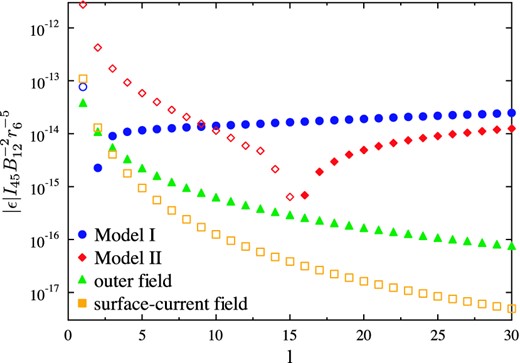
Figure 1.
The effective oblateness ϵ calculated for different axisymmetric (m = 0) poloidal harmonics calculated with different magnetic field configuration models. Here, I45 = I*/1045 g cm2. Filled markers correspond to negative values of ϵ, hollow ones to positive values of ϵ. If one wants to obtain the oblateness produced by non-axisymmetric harmonics, the corresponding value should be multiplied by (l2 + l − 3m2)/(l2 + l).
The effective oblateness calculated with Model II remains negative up to l = 15. To understand this behaviour, we should point out that, according to the expressions (18) and (19), radial field component Bn ∝ Rl, while tangential field component Bt ∝ drRl. Thus, expression (32) can be interpreted in such a way that the radial and tangential components generate oppositely directed torques. For small l, most of the crust volume is occupied by a tangential field (see Fig. 2). With growing l, the crust field becomes more and more vertical. The radial and tangential field component contributions are approximately equal for a magnetic field cell with radius equal to the crust thickness. For hc = 0.1r*, this takes place between l = 15 and 16. Harmonics with l > 16 give oblateness values that tend to the corresponding results calculated with Model I. The reason for this is that the form of the magnetic field cells in the two models becomes more and more similar with increasing l.
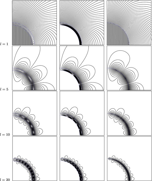
Figure 2.
Magnetic field lines: Model I (left), Model II (centre) and surface-current model (right).
One can see that for high harmonics the absolute value of effective oblateness increases slightly with l. The boundary conditions for radial function derivatives at the star surface and crust–core interface require an increase of the derivatives and the function itself inside the crust with increasing l (see Fig. 3). Physically, this means that the same magnetic field magnitude at the star surface requires a stronger field inside the crust in the case of a more small-scale field. The first integral in expression (32) grows slightly with l, because of the boundary conditions, while the pre-integral factor tends to a constant. Note, however, that this slight growth of |ϵ| is the consequence of the choice of harmonics normalization. If, for example, we calculate |$\boldsymbol{K}_\perp$| fixing the maximum value of the surface magnetic field instead of |$\langle B^2\rangle _{r_*}$|, an additional factor (l + 1) in the denominator of (32) arises, leading to the decrease of |ϵ| with increasing l.
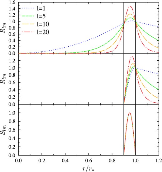
Figure 3.
Radial functions of the poloidal field: Model I (top panel), Model II (middle panel) and toroidal field model (bottom panel).
In order to demonstrate the importance of the finite thickness of the crust (magnetic-field generating layer), we have also considered the surface-current model:
(right panel in Fig.
2). The presence of a surface current leads to the breaking of boundary condition (
21) and discontinuity of the magnetic field tangential component. For such a field configuration, the effective oblateness decreases with
l even faster than the oblateness produced only by an outer field. It is a consequence of the fact that the external and internal fields produce contributions to δ
If of opposite sign and the terms containing the largest power of
l cancel each other.
A toroidal component of
|$\boldsymbol{B}_0$| can exist inside the star. The anomalous torque produced by a single toroidal harmonic has the form
where again vector
|$\boldsymbol{k}$| equals (
33). The toroidal harmonics cannot be normalized at the surface field value. We normalize them at the volume-averaged field:
where
r0 is the lower boundary of the region occupied by the toroidal field.
We chose the toroidal radial functions to be equal to
where
b is the normalization constant. Again, functions
Slm are the eigenmodes of free Ohmic decay, but satisfying toroidal field boundary condition (
22). There is no single point of view about how large the region occupied by the toroidal magnetic field is. However, according to modern researches (Braithwaite & Nordlund
2006; Ciolfi et al.
2009), the most realistic field configuration corresponds to a toroidal field confined in a region of poloidal field lines closed in the star interior. In the poloidal field models considered by us, such lines exist only inside the crust (see Fig.
2), so we set
r0 =
rc. Hence, coefficients μ
l are obtained as the roots of equation
Slm(
rc) = 0. Again, for each index
l we take the smallest root, corresponding to the most long-lived eigenmode. One can see from Fig.
3 that the radial functions chosen in this way are almost indistinguishable, despite the index
l running from 1 to 20. This fact does not seem completely unexpected related bell-shaped functions fixed at two closely spaced points and normalized at unity at their maximum.
Thus, for our chosen model, the integrals in expression (
41) barely depend on
l and the effective oblateness produced by a single axisymmetric harmonic is almost independent of
l as well. It equals
where
|$B_{V12} = \sqrt{\langle B^2\rangle _V}/10^{12}$| G. In the case of non-axisymmetric harmonics, one needs to multiply (
44) by (
l2 +
l − 3
m2)/(
l2 +
l). Note that the toroidal field may be 1–2 orders of magnitude stronger than the poloidal field (Braithwaite
2009). If so, it gives a leading contribution to the anomalous torque.
If a star's magnetic field is defined by several spherical harmonics, the anomalous torque does not equal the sum of contributions of each of these harmonics in the general case. Considering a poloidal magnetic field constructed from two harmonics, one sees that the cross-term under integral (9) can be represented as the sum of products |$(\boldsymbol{e}_i\cdot \boldsymbol{e}_r)Y_{lm}(\boldsymbol{e}_j\cdot \boldsymbol{e}_r)Y_{l^{\prime }m^{\prime }}$| and |$(\boldsymbol{e}_i\cdot \nabla Y_{lm})(\boldsymbol{e}_j\cdot \nabla Y_{l^{\prime }m^{\prime }})$|, where i, j = x, y, z. According to the handbook of Varshalovich, Moskalev & Khersonskii (1988), combinations |$(\boldsymbol{e}_i\cdot \boldsymbol{e}_r)Y_{lm}$| and |$(\boldsymbol{e}_i\cdot \nabla Y_{lm})$| can be expressed through sums of the spherical functions Yl ± 1; m and Yl ± 1; m ± 1. This means that only the cross terms between the l and l ± 2 poloidal harmonics survive after integrating over all directions. The cross term between two toroidal harmonics consists of products |$(\boldsymbol{e}_i\cdot [\nabla \times \nabla Y_{lm}])(\boldsymbol{e}_j\cdot [\nabla \times \nabla Y_{l^{\prime }m^{\prime }}])$|. These combinations, according to the same handbook, are represented through the sum of spherical functions Yl; m and Yl; m ± 1. Hence, toroidal harmonics with different index l do not cross at all.
There are several articles where the anomalous torque has been calculated by different methods, mostly assuming that the magnetic field consists of a single poloidal dipolar harmonic (Davis & Goldstein
1970; Good & Ng
1985; Melatos
2000; Istomin
2005; Beskin & Zheltoukhov
2014). The anomalous torque can be obtained by direct integration of the Lorentz force over the star volume (Good & Ng
1985; Beskin & Zheltoukhov
2014):
This method is more straightforward but more complex, because one needs to calculate second-order corrections to the fields. Another approach is to use the formula for the angular momentum flux (Melatos
2000):
where, in contrast to formula (
12), averaging is performed over the star surface. However, by analogy with equation (
1), this flux equals the variation of the star's angular momentum plus the angular momentum of the internal field. Thus, the internal field does not contribute to the anomalous torque calculated with formula (
46). It should be accounted for in the star's angular momentum. Beskin & Zheltoukhov (
2014) proposed a modification of this formula, taking into account the internal field but applicable when the star magnetic field is generated only by surface currents. Since almost all authors have assumed a vacuum magnetosphere [relation (
3) is not satisfied outside the star], a direct comparison of our results with others cannot be made. Only Good & Ng (
1985) assumed a particle-filled magnetosphere. They used the same method and obtained the same result, but restricted themselves to dipolar and quadrupolar poloidal harmonics and a surface field model.
3 EFFECTIVE INERTIA TENSOR
We have argued that neutron star magnetic fields of different scales may give comparable contributions to the anomalous torque. Further, we would like to discuss the consequences that may result from possible deviation of the magnetic field from a pure dipolar configuration. Let us consider the simplest model of ‘asymmetric’ anomalous torque:
Here, the first term is produced by the dipolar field,
|$\boldsymbol{e}_{m} = \boldsymbol{m}/m$|, where
|$\boldsymbol{m}$| is the dipolar moment vector. The second term is produced by some other field component. It can be, for example, a quadrupole field, the axis of which does not coincide with
|$\boldsymbol{e}_m$|, or some small-scale field anomaly. Here,
|$\boldsymbol{e}_{s}$| is some unity vector that does not coincide with
|$\boldsymbol{e}_{m}$|. Let us introduce angle α, the cosine of which is given by
|$\cos \alpha = (\boldsymbol{e}_{s} \cdot \boldsymbol{e}_{m})$|.
In the case of a perfectly spherical star, equation (
14) can be rewritten as
Recall that coefficients δ
Idip and δ
Is are many orders of magnitude smaller than the star moment of inertia
I*. If one substitutes torque (
47) into equation (
48) and adds negligibly small terms
|$\delta I_{\rm dip}\left({\rm d}_t{\boldsymbol{\Omega }}\cdot \boldsymbol{e}_{m}\right)\boldsymbol{e}_m$| and
|$\delta I_{s}\left({\rm d}_t{\boldsymbol{\Omega }}\cdot \boldsymbol{e}_{s}\right)\boldsymbol{e}_{s}$| to the left-hand side, the equation can be reduced to compact form:
where
|${\rm d}_t^*$| is the time derivative in the frame of reference rotating with the star
|$M_{\rm eff}^i = I_{\rm eff}^{ij}\Omega ^j$| and we have introduced an effective inertia tensor
Writing
|$I_{\rm eff}^{ij}$|, we use an orthonormal basis
|$(\boldsymbol{e}_{x^{\prime }},\boldsymbol{e}_{y^{\prime }},\boldsymbol{e}_{z^{\prime }})$| fixed in the star in such a way that
|$\boldsymbol{e}_{z^{\prime }} = \boldsymbol{e}_m$| and
|$\boldsymbol{e}_{x^{\prime }}$| lies in the plane containing
|$\boldsymbol{e}_m$| and
|$\boldsymbol{e}_{s}$| (see Fig.
4). Tensor (
50) can be diagonalized by turning this basis at angle β (see Fig.
4):
The corresponding eigenvalues are
As a result, the rotation of a spherical neutron star under the action of anomalous torque can be described as the free rotation of a triaxial star.

Figure 4.
Two orthonormal bases used in Section 3: |$(\boldsymbol{e}_{x^{\prime }},\boldsymbol{e}_{y^{\prime }},\boldsymbol{e}_{z^{\prime }})$| is the basis related to the magnetic dipole, while |$(\boldsymbol{e}_{x},\boldsymbol{e}_{y},\boldsymbol{e}_{z})$| is the basis in which tensor |$I_{\rm eff}^{ij}$| is orthogonal.
In the general case, the anomalous torque produced by a magnetic field cannot be represented in form (47), as it contains more terms. This means that tensor |$I_{\rm eff}^{ij}$| has a form more complicated than (50) and requires a more complicated procedure to find the effective principal axes, but the idea remains the same.
Real neutron stars are not perfectly spherical in themselves. First, their form is deformed by the stresses produced by their own internal magnetic field (Wasserman 2003; Haskell, Samuelsson, Glampedakis & Andersson 2008; Mastrano et al., 2011; Mastrano, Lasky & Melatos 2013). Secondly, non-hydrostatic deformations can be maintained by star's solid crust (Goldreich 1970). In the general case, tensor |$I_{\rm eff}^{ij}$| can be obtained by summation of the triaxial star inertia tensor and the tensor describing the inertia of the near-zone field.
4 EQUATIONS OF MOTION
Let us return to the angular momentum balance equation,
Here,
|$\boldsymbol{M}_{\rm eff}$| is the effective angular momentum vector of general form. Now we add to the equation the ‘external’ torque
|$\boldsymbol{K}_3$|, which is the next term of electromagnetic torque expansion in a series of small parameter ε (
|$\boldsymbol{K}_3\propto \varepsilon ^3$|). Despite its smallness compared with the anomalous torque (included here in term
|$\boldsymbol{\Omega }\times \boldsymbol{M}_{\rm eff}$|), torque
|$\boldsymbol{K}_3$| is important when the long-term rotation dynamics is considered, because only the torque proportional to ε
3 causes star spin-down and secular inclination angle evolution. The rotation of a triaxial star under the action of ‘external’ electromagnetic torque was studied by Melatos (
2000). In this section, we will discuss some key points regarding such rotation.
If
|$\boldsymbol{e}_m \ne \boldsymbol{e}_\Omega$|, an arbitrary torque
|$\boldsymbol{K}_3$| can be represented as (Barsukov, Polyakova & Tsygan
2009)
where
|$\mathcal {K} = \varepsilon ^3 m^2/r_*^3$| and
|$\tilde{k}_\Omega$|,
|$\tilde{k}_m$|,
|$\tilde{k}_p$| are some dimensionless functions. Since we suppose that
|$\boldsymbol{K}_3$| is caused only by rotation of magnetic dipole moment
|$\boldsymbol{m}$|, this representation is most convenient. Moreover, since
K ∼ ε
3, even if function
|$\tilde{k}_p$| does not equal zero, this term, being parallel to the dipolar contribution to anomalous torque, is much smaller than
K⊥. It allows us to ignore the last term in expression (
56). In contrast to the anomalous torque, the exact form of torque
|$\boldsymbol{K}_3$| is difficult to obtain because its calculation requires knowledge of field behaviour not only near the star but up to a distance ∼
rL. For this reason, researchers use different model torques (Davis & Goldstein
1970; Jones
1976; Beskin, Gurevich & Istomin
1983; Barsukov, Polyakova & Tsygan
2009).
Since both effective and real deformations are very small, one can replace
|${\rm d}_t^*{\boldsymbol{M}}_{\rm eff}$| by
|$I_* {\rm d}_t^*{\boldsymbol{\Omega }}$| in equation (
55) (see the Appendix for more detail). After substitution of expression (
56), this vector equation can be represented as the following three equations:
Here, ϑ and φ (not to be confused with θ and ϕ) are precession and azimuthal angles, defined as shown in Fig.
5,
are the oblateness parameters,
|$\cos \chi = \left(\boldsymbol{e}_\Omega \cdot \boldsymbol{e}_m\right)$| is the cosine of inclination angle χ,
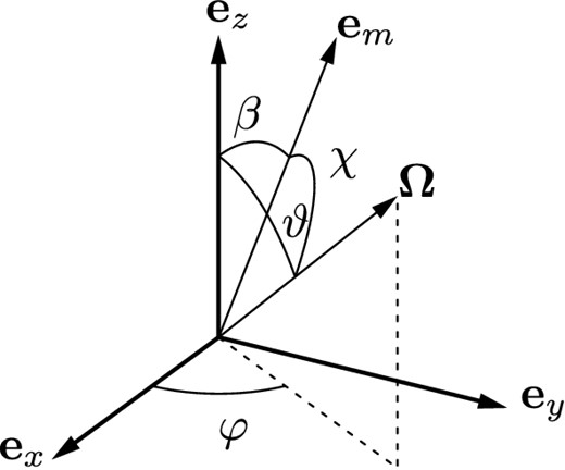
Figure 5.
Angles and vectors used in Section 4: |$\boldsymbol{e}_x$|, |$\boldsymbol{e}_y$|, |$\boldsymbol{e}_z$| are the principal axes of the star effective inertia tensor |$I_{\rm eff}^{ij}$|, β is the angle between the Z-axis and the star's magnetic moment direction, ϑ is the precession angle and χ is the inclination angle.
Let us first consider ‘free’ rotation (|$\mathcal {K} = 0$|). In the case of an effectively triaxial star, the angular velocity vector can rotate about two of three effective principal axes, corresponding to the largest and smallest principal moments of inertia depending on the initial conditions. If the angular velocity vector rotates about the z-axis, angles ϑ and φ have a simple intuitive meaning. The variation of angle φ describes the precessional motion of the star. The ‘amplitude’ of the precession is set by angle ϑ. Oscillations of angle ϑ describe the nutation of the star. The amplitude of these oscillations is proportional to (ϵy − ϵx) (see the Appendix). Note that we introduce ϑ as the angle between the angular velocity vector and the principal axis of the effective inertia tensor, while Melatos (2000) measures this angle between |$\boldsymbol{\Omega }$| and the principal axis of the body inertia tensor.
Using formula (
A11), one can estimate the precession period:
where
P is the period of neutron star rotation and
f ∼ 1 is a coefficient calculated with (
A12). The observed parameter is the inclination angle χ. It oscillates with the same period
Tp.
If we now include in the consideration torque
|$\boldsymbol{K}_3$|, another evolution time-scale,
arises. It is usually much larger than the precession period
Tp. As it was shown by Goldreich (
1970), the ‘external’ torque can both damp the precession and increase its amplitude, depending on the orientation of dipole moment
|$\boldsymbol{m}$| relative to the star's principal axes. He considered an axisymmetric neutron star (ϵ
x = ϵ
y), the magnetic moment
|$\boldsymbol{m}$| of which departs from the star's symmetry axis
|$\boldsymbol{e}_z$| at angle β, so that cos χ = cos βcos ϑ + sin βsin ϑcos φ and
|$\left( \boldsymbol{e}_\vartheta \cdot \boldsymbol{e}_m \right) = - \cos \beta \sin \vartheta + \sin \beta \cos \vartheta \cos \varphi$|. He also assumed that the star loses its angular momentum due to magneto-dipolar radiation (Davis & Goldstein
1970):
Being interested in the secular evolution of angle ϑ, one can average equation (
58) over the precession period, substituting in the right-hand side the free precession solution Ω, ϑ = const, φ = 2π(
t/
Tp). After averaging, one can verify that
|$\langle \left(\boldsymbol{e}_\vartheta \cdot \boldsymbol{e}_m \right)\tilde{k}_m\rangle _{T_{\rm p}}$| is negative for
|$\beta < \arccos (3^{-{1}/{2}}) \approx 55^\circ$| and positive for β > 55°. This means that the amplitude of precession decreases if β < 55° and increases in the opposite case. It is obvious that the critical angle is the same for any model of torque
|$\boldsymbol{K}_3$|, in which
|$\tilde{k}_m\propto \cos \chi$|. However, if the proportionality factor is negative, the situation is opposite: the precession is damped if β > 55° and it grows if β < 55°. This should take place, for example, for a current losses model (Beskin et al.
1983).
Note that Goldreich (1970) ignored the anomalous torque in his calculations. This is correct only if the star deformation is much larger than the effective oblateness produced by the inertia of the field. In the general case, one should take into account both asymmetries of the star and its field inertia distribution. Therefore, even an axisymmetric star effectively becomes triaxial if the magnetic moment direction does not coincide with the star symmetry axis. For such a star, the question of whether the amplitude of precession would increase or decrease is more complex. It depends on the relation between ϵx and ϵy, as well as on the initial conditions.
Typical curves of angles evolution with damped precession are shown in Fig. 6. In plotting these graphs, we assumed that the star is spherical and obtained oblateness parameters (60) using |$I_{\rm eff}^{xx}$|, |$I_{\rm eff}^{yy}$| and |$I_{\rm eff}^{zz}$| calculated with formulae (52)–(54) and the following parameters: α = 30°, |$\delta I_{\rm dip} = 0.36 \mathcal {K} (c /r_* \Omega ^3)$| and δIs = 1.2δIdip. Time is measured in units of τx. It makes the curves independent of I* and, if ϵx and ϵy are proportional to m2, of neutron star magnetic field strength. The form of the angles oscillations envelope also does not depend on the initial period in these time units. However, initial precession period Tp/τx ∝ Ω0. Since ϵy ≈ ϵx for this configuration, oscillations of ϑ are small (they are almost indistinguishable in the graph). However, the inclination angle χ oscillates with amplitude ≈30° at the beginning of the evolution. Individual oscillations of angle χ are indistinguishable because of the small precession period compared with τx.
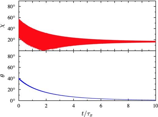
Figure 6.
Evolution of inclination angle χ and precession angle ϑ with time for a pulsar with the following parameters: |$\epsilon _x = 1.9\times 10^{-13} I_{45}^{-1}$|, |$\epsilon _y = 2.05\times 10^{-13} I_{45}^{-1}$|, β = 16.5° and for the following initial conditions: P0 = 0.1s, ϑ0 = 40°, φ0 = 45°. Time is measured in evolution time-scales τx.
The form of the inclination angle oscillations envelope can be understood after looking at Fig. 7. While ϑ > β, the inclination angle changes from ϑ − β to ϑ + β during the precession period, so that the amplitude is constant and equal to 2β. After angle ϑ becomes less than β, the inclination angle starts to change from β − ϑ to ϑ + β. This means that the amplitude equals 2ϑ and consequently decreases with the damping of precession.
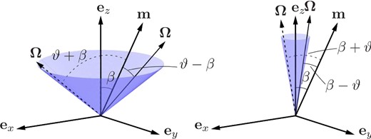
Figure 7.
Precession motion of angular velocity vector |$\boldsymbol{\Omega }$| for the cases ϑ > β (left panel) and ϑ < β (right panel). The opening of the precession cones is equal to 2ϑ.
Plotting these curves, we used the vacuum magneto-dipolar formula (64). Modern magnetohydrodynamics simulations of pulsar magnetospheres (Philippov, Tchekhovskoy & Li 2014) yield a torque causing slower secular inclination angle evolution, but qualitatively the behaviour of the curves is the same.
It is important to note that, due to anomalous torque after the damping of precession, the star will not rotate about one of its own principal axes but about one of the effective principal axes. This is why the precession angle measured by Melatos (2000) from the body principal axis in some of his simulations tends to a finite constant.
Another scenario of angle evolution is shown in Fig. 8. In this example, the precession grows with time. Here, the difference between ϵx and ϵy is much larger and the oscillations of angle ϑ are much more noticeable. At approximately t/τx = 4, angle ϑ reaches 90° and the star changes its axis of precession from |$\boldsymbol{e}_z$| to |$\boldsymbol{e}_x$|. After that, angle ϑ loses the meaning of a ‘precession angle’.
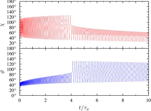
Figure 8.
Evolution of inclination angle χ and precession angle ϑ with time for a pulsar with the following parameters: |$\epsilon _x = 2.06\times 10^{-13} I_{45}^{-1}$|, |$\epsilon _y = 1.13\times 10^{-13} I_{45}^{-1}$|, β = 79° and for the following initial conditions: P0 = 0.1 s, θ0 = 40°, φ0 = 45°. Time is measured in evolution time-scales τx.
A full analysis of triaxial star rotation under the action of a torque of the form (56) is quite complex: both ϵx and ϵy can be both positive and negative, the absolute value of ϵx can be either larger or smaller than the absolute value of ϵy, function |$\tilde{k}_m$| can be either positive or negative depending on the magnetosphere model, vector |$\boldsymbol{m}$| can be arbitrarily oriented with respect to the principal axes and so on. One of the essential assumptions that was made is that the neutron star rotates as a perfectly rigid body. In reality, a number of dissipation processes accompany the precession motion. Examples are crust internal friction (Chau & Henriksen 1971; Macy 1974), crust–core friction (Chau & Henriksen 1971; Casini & Montemayor 1998), mutual friction between neutron superfluid vortices and a charged component (Sedrakian, Wasserman & Cordes 1999) and so on. At the very least, the growing precession should be discussed only after dissipation processes are taken into consideration. We did not aim to perform such analysis here.
5 CONCLUSIONS
In this article, we have calculated the so-called anomalous torque produced by different poloidal and toroidal magnetic field harmonics. It is shown that small-scale field structures may give a contribution to this torque comparable in magnitude with the contribution of dipolar field. The magnitude of the torque may depend substantially on the internal field structure. If the star magnetic field is not symmetric with respect to the dipolar moment axis, the pulsar inclination angle may oscillate with a typical amplitude of tens of degrees, due to precession. Such variations may in principle be observable (Lyne et al. 2013).
Besides the anomalous torque, the magnetic field should deform neutron stars directly. However, this effect is more difficult to calculate and may depend substantially on the neutron star equation of state (Haskell et al. 2008). For arbitrary poloidal harmonics, the star deformation was calculated by Mastrano et al. (2013). Formally, their results are much larger than the effective oblatenesses obtained by us. However, they used another internal field model. This difference is especially important for large l: for the same harmonic and same surface field strength, their field can be up to one order of magnitude larger inside the star (both direct deformation and anomalous torque are quadratic in B) than the field we assume in our models. Moreover, according to their model small-scale fields occupy the whole star, while we assume that these fields are concentrated in the crust. Thus, direct comparison of the corresponding oblateness coefficients does not give a real picture of the relative contributions of these two effects.
The neutron star core in some regions may be in a superconducting state (Yakovlev, Levenfish & Shibanov
1999). If it is a superconducting state of the first kind, the magnetic field is pushed out of the core and the field configuration may be like that we propose in
Model II. If, however, the superconductivity is of the second kind, the field is organized in fluxoids, which can be modelled as cylindrical tubes with radius approximately equal to penetration depth Λ and filled with the first critical field
Hc1 ≈ 4 × 10
14(ρ/10
14g cm
−3) G directed along the tube axes (Glampedakis, Andersson & Samuelsson
2011). Let us consider a small box with size ℓ and volume
V = ℓ
3. The inertia of the field contained in this box can be estimated roughly as the field energy multiplied by the distance from a principal axis and divided by the speed of light. For the energy, we have
where
N is the number of flux tubes contained in the box and by
BV we mean the field averaged over this small volume. Thus, in the case of a superconducting interior, we expect an increase in the internal part of
|$\boldsymbol{K}_\perp$| by a factor ∼
Hc1/
BV.
The authors thank A. A. Zheltoukhov and V. S. Beskin for the discussions that led to the initial idea for this article. The authors are also grateful to M. Rheinhardt for many useful comments. The work of AIT was partly supported by the Russian Foundation for Basic Research (project 13-02-00112).
REFERENCES
Astron. Rep.
2009
53
1146
Astronomy and Astrophysics Library, MHD Flows in Compact Astrophysical Objects: Accretion, Winds and Jets
2009
Berlin
Springer-Verlag
Sov. J. Exper. Theor. Phys.
1983
58
235
Phys. Uspekhi
2014
57
865
Astrophys. Lett.
1971
8
49
Progress in Neutron Star Research Magnetodipole Oven
2005
New York
Nova Science Publishers Inc.
27
The Classical Theory of Fields, Course of Theoretical Physics
1975
Linacre House, Jordan Hill, Oxford
Butterworth Heinemann
Quantum Theory of Angular Momentum: Irreducible Tensors, Spherical Harmonics, Vector Coupling Coefficients, 3nj Symbols
1988
Singapore
World Scientific Press
Phys. Uspekhi
1999
42
737
APPENDIX A: FREE MOTION OF AN ASYMMETRICAL TOP
Let us consider a rigid body rotating with angular velocity
|$\boldsymbol{\Omega }$|. If this body does not feel the action of any forces, its energy
and three components of angular momentum
are conserved. The angular conservation law can be represented in the form of equation
where
|${\rm d}_t^*$| denotes the time derivative in the frame corotating with the body. Since the inertia tensor is symmetrical, one can always find a corotating basis
|$(\boldsymbol{e}_x,\boldsymbol{e}_y,\boldsymbol{e}_z)$| in which this tensor is diagonal. Projected on to this basis, equation (
A3) is equivalent to three Euler's equations:
By a cyclic change of vectors
|$\boldsymbol{e}_i$|, one can rearrange the principal moments of inertia so that
Ixx ≤
Iyy ≤
Izz.
If
M2 > 2
EIyy, the system of equations (
A4)–(
A6) has the following solution (Landau & Lifshitz
1975):
where cn
k(τ), sn
k(τ) and
|${\rm dn}_k(\tau ) = \sqrt{1-k^2{\rm sn}_k(\tau )}$| are the Jacobi elliptic functions, with parameter
ranging from 0 to 1 and argument τ = 2π
f(
t/
Tp), where
and
Functions cn
k(τ) and sn
k(τ) are periodic, with period 2π
f. In terms of physical time, this period equals
Tp. For
k = 0, the elliptic functions reduce to trigonometric functions: sn → sin , cn → cos , dn → 1. For
k = 1, they reduce to hyperbolic functions: sn → tanh , cn, dn → 1/cosh .
Instead of Cartesian components, vector
|$\boldsymbol{\Omega }$| can be described by its absolute value
|$\Omega = \sqrt{\Omega ^x\Omega ^x+\Omega ^y\Omega ^y+\Omega ^z\Omega ^z}$| and two angles: precession angle
|$\vartheta = \arccos (\Omega ^z/\Omega )$| and azimuthal angle
|$\varphi = \arcsin (\Omega ^y/\sqrt{\Omega ^x\Omega ^x+\Omega ^y\Omega ^y})$|. It is also convenient to introduce two oblateness parameters, ϵ
x = (
Izz −
Ixx)/
Izz and ϵ
y = (
Izz −
Iyy)/
Izz, which are both positive. Using solution (
A7)–(
A9) and definitions (
A1) and (
A2), one can obtain
where Ω
0 and ϑ
0 are the initial values of Ω and ϑ and angle φ
0 is supposed to be equal to zero.
If Ixx = Iyy (ϵx = ϵy, k = 0), Ω and ϑ remain constant and vector |$\boldsymbol{\Omega }$| rotates uniformly about the z-axis. If vector |$\boldsymbol{e}_z$| is directed at us, this rotation is counterclockwise. In the general case, the absolute values of angular velocity Ω and precession angle ϑ oscillate with doubled frequency.
Our interest is restricted to rotation of a body in which the mass distribution is almost spherically symmetric (i.e. ϵ
x, ϵ
y ≪ 1). In this case, one can ignore all terms quadratic in ϵ
x, ϵ
y in equations (
A4)–(
A6). This is equivalent to replacing equation (
A3) by the equation
It is easy to see that, in this approximation, the variation of angular velocity
|$\boldsymbol{\Omega }$| is perpendicular to this vector. Indeed, looking at expression (
A13), one can see that oscillations of the absolute value of angular velocity are quadratically small in terms of oblateness parameters. As for angle ϑ, if the body is substantially triaxial, i.e. (ϵ
x − ϵ
y)/ϵ
y ∼ 1, its oscillations can be not small even for an almost spherical body.
If M2 < 2EIyy, the solution to equations (A4)–(A6) can be obtained from the one discussed above by exchanging ‘x’↔ ‘z’. This means that, in this case, vector |$\boldsymbol{\Omega }$| rotates about the x-axis. Measuring φ from the z-axis, we should keep in mind that |$(\boldsymbol{e}_z,\boldsymbol{e}_y,\boldsymbol{e}_x)$| is left-handed triple. Hence, in contrast to rotation about the z-axis, this rotation is clockwise.
© 2015 The Authors Published by Oxford University Press on behalf of the Royal Astronomical Society


