


Abstract
In this paper, we attempt to investigate the nature of the first gravitational wave (GW) signal to be detected by pulsar timing arrays (PTAs): will it be an individual, resolved supermassive black hole binary (SBHB), or a stochastic background made by the superposition of GWs produced by an ensemble of SBHBs? To address this issue, we analyse a broad set of simulations of the cosmological population of SBHBs that cover the entire parameter space allowed by current electromagnetic observations in an unbiased way. For each simulation, we construct the expected GW signal and identify the loudest individual sources. We then employ appropriate detection statistics to evaluate the relative probability of detecting each type of source as a function of time for a variety of PTAs; we consider the current International PTA, and speculate into the era of the Square Kilometre Array. The main properties of the first detectable individual SBHBs are also investigated. Contrary to previous work, we cast our results in terms of the detection probability (DP), since the commonly adopted criterion based on a signal-to-noise ratio threshold is statistic-dependent and may result in misleading conclusions for the statistics adopted here. Our results confirm quantitatively that a stochastic signal is more likely to be detected first (with between 75 and 93 per cent probability, depending on the array), but the DP of single-sources is not negligible. Our framework is very flexible and can be easily extended to more realistic arrays and to signal models including environmental coupling and SBHB eccentricity.
1 INTRODUCTION
Our current knowledge of the Universe is almost entirely based on electromagnetic observations (from radio waves, up to gamma rays). A direct gravitational wave (GW) detection will open an alternative and complementary perspective on the Cosmos (Sathyaprakash & Schutz 2009). According to General Relativity, accelerating masses with a mass quadrupole moment varying in time generate GWs, and our Universe has plenty of systems fulfilling such a requirement (Wald 1983; Maggiore 2008); from compact binaries (emitting GWs while inspiraling towards one another until coalescence; Peters & Mathews 1963), to asymmetric spinning compact stars (Van Den Broeck 2005), and catastrophic supernovae explosions (Yakunin et al. 2010), just to mention a few.
A direct GW detection is a long-standing challenge in experimental physics, dating back to the 60's. To date, two different approaches to the problem have polarized the attention of the scientific community, bringing the promise of the first direct GW detection. One technique is ground based laser interferometry; the second generation of ground based detectors (GBDs), including advanced LIGO (LIGO Scientific Collaboration 2009), advanced Virgo (Accadia et al. 2012) and KAGRA (Somiya 2012), will soon be online, and is expected to observe tens of coalescing neutron star or stellar-mass black hole binaries (Abadie et al. 2010). The other technique consists of timing an ensemble of ultrastable millisecond pulsars, forming what is commonly referred to as a pulsar timing array (PTA). The times of arrival (ToAs) of radio pulses emitted by galactic millisecond pulsars are collected by 100-m class radio telescopes around the globe. Since these pulses are so extremely regular, a GW passing by would introduce irregularities in their ToAs, a detectable fingerprint that can be measured, provided 100 ns timing precision is achieved on a large number of pulsars (Sazhin 1978; Detweiler 1979; Hellings & Downs 1983). Regardless of which approach, either GBDs or PTAs, achieves a GW detection first, the two independent detections are necessary, because they target orthogonal classes of sources, therefore providing complementary information about the Universe. The invaluable scientific promises of GW astronomy are potentially so revolutionary that the design of a third generation of GBDs – the Einstein telescope (ET) – is now being investigated (Punturo et al. 2010), and the European Space Agency (ESA) has selected The Gravitational Universe science theme (eLISA Consortium et al. 2013) for the L3 launch slot, with eLISA – the evolved laser interferometer space antenna – put forward as strawman mission design, now scheduled for 2034.
Within the LIGO Scientific Collaboration1, different groups have formed in order to specialize in the detection of the four different types of expected GW signals: (i) a stochastic GW background (GWB; LIGO Scientific Collaboration & Virgo Collaboration 2014c), (ii) continuous waves (LIGO Scientific Collaboration & Virgo Collaboration 2014b), (iii) bursts (LIGO Scientific Collaboration & Virgo Collaboration 2014a), and (iv) compact binary coalescences (aka CBC, LIGO Scientific Collaboration & Virgo Collaboration 2013). A GWB is the superposition of numerous similar GW sources, adding up in an incoherent fashion, and can have either an astrophysical origin, e.g. coming from a large population of a specific class of astrophysical objects (Regimbau 2011; Rosado 2011), or cosmological, e.g. coming from physical processes such as inflation or phase transitions in the early Universe (Allen 1997; Maggiore 2000). Continuous waves are quasi-sinusoidal signals, expected to be produced by rotating neutron stars. The burst search targets short GW transients (≲1 s) with limited assumptions on the waveform. On the contrary, the CBC search relies on accurate models for the waveform emitted by coalescing binaries, and seeks for patterns in the detector's data that match such models.
PTAs are following a similar path, but maintain a flexible structure. There are three independent PTA consortia: the European PTA (EPTA; Ferdman et al. 2010), the Parkes PTA (PPTA; Manchester et al. 2013), and NANOGrav (Jenet et al. 2009). The three groups join forces and combine data under the aegis of the International PTA (IPTA; Hobbs et al. 2010), which is formally a consortium of consortia. The main target of PTA campaigns are the GWs emitted by supermassive black hole (SBH) binaries (SBHBs; see e.g. Sesana, Vecchio & Colacino 2008), although processes in the early Universe may also produce GWs in the same frequency band, like cosmic strings (Sanidas, Battye & Stappers 2012) or the cosmological QCD phase transition (Caprini, Durrer & Siemens 2010).
On the basis of the hierarchical paradigm of structure formation – according to which galaxies we see today underwent a series of merger events (White & Rees 1978) – and on the observational fact that SBHs are ubiquitous in galaxy centres (e.g. Magorrian et al. 1998), following galaxy mergers, a vast number of SBHBs is expected to form along the cosmic history (Begelman, Blandford & Rees 1980). Although there is plenty of observational evidence of the existence of SBH pairs separated by hundreds-to-thousands of parsecs, detecting parsec and subparsec scale SBHBs driven by GWs has been proven challenging, and only candidate systems supported by circumstantial evidence have been proposed to date (see Dotti, Sesana & Decarli 2012, for an extensive review on the topic). The recent access to vast time domain optical data set resulted in the discovery of a number of quasars showing periodic variability (Graham et al. 2015; Liu et al. 2015), but the SBHB nature of these objects is difficult to prove. In any case, a large population of SBHBs is an inevitable prediction of current galaxy formation models, and their GW signals must have travelled to our galaxy imprinting their signature in the pulsars’ ToAs. The incoherent superposition of many signals will possibly result in a stochastic GWB (Rajagopal & Romani 1995), but particularly massive and/or nearby SBHBs might dominate the signal budget and show up as resolvable continuous waves (Sesana, Vecchio & Volonteri 2009) in the data. Moreover, bursts from particularly eccentric binaries (Amaro-Seoane et al. 2010; Finn & Lommen 2010) or from the GW memory effect (Favata 2009; Pshirkov, Baskaran & Postnov 2010; van Haasteren & Levin 2010) are also possible. Consequently, several IPTA projects have been established, targeting different types of signals. Unlike GBDs, there are no CBC searches within the PTA, since SBHBs are observed long before coalescence, during their slow, adiabatic inspiral. For PTAs, the first detection will probably be either a continuous wave signal from an SBHB (we will refer to such signal as a ‘single source’ from now on) or a GWB, and we focus on these two classes of sources in this study.
A GWB is commonly characterized by an amplitude and a spectral slope (Jenet et al. 2005). Detecting a GWB, with amplitude and slope consistent with the expected signal generated by an ensemble of SBHBs, would prove the validity of the models that predict the existence of tight SBHBs, and, in a broader context, would support our current understanding of the formation and evolution of galaxies. Moreover, the detection of a GWB could put constraints on alternative theories of gravity, or prove their validity against General Relativity (Chamberlin & Siemens 2012). However, an ensemble of SBHBs could also produce a spectrum different than a simple power law (Sesana et al. 2004; Kocsis & Sesana 2011; Sesana 2013a; McWilliams, Ostriker & Pretorius 2014; Ravi et al. 2014), and other GW sources could also lead to different measurable GWBs; detecting the actual shape of the GWB would help discriminate between these different models (Sampson, Cornish & McWilliams 2015).
The detection of a single SBHB (Corbin & Cornish 2010; Yardley et al. 2010; Ellis 2013; Wang, Mohanty & Jenet 2014) would allow for some further appealing prospects. First, by detecting a purely stochastic GWB one cannot, in principle, be sure of the kind of sources that originated it; however, detecting a single SBHB would be a more direct proof of the existence of tight binaries. Detecting a single source would allow us to measure the characteristics of the binary, for example its luminosity distance, mass, orbital period, and sky location, opening fascinating prospects for multimessenger astronomy (Sesana et al. 2012; Tanaka, Menou & Haiman 2012; Burke-Spolaor 2013; Rosado & Sesana 2014). In some cases, it could also help to improve our measurement of the distance to the pulsars in the array (Lee et al. 2011).
Although it is commonly believed that a GWB detection will likely precede the identification of any single source, this statement has never been properly quantified in the literature. The aim of this paper is precisely to answer the question: what type of signal will more likely be detected first by a PTA, and with what probability? To tackle the problem, we analyse a large set of simulated realizations of the ensemble of SBHBs, and compare the detectability of the two types of signals as a function of time in each of them. The realizations are produced following the prescriptions of Sesana (2013b), employing, for this exploratory study, the simplifying assumption of circular, GW-driven binaries.
The outline of the paper is as follows. In Section 2, we describe the simulations of the SBHB cosmic population and present the necessary mathematical tools to evaluate the detectability of the GWB and of single SBHBs; finally, we describe the properties of the pulsar arrays assumed as GW detectors. In Section 3, the detection probability (DP) of the GWB is compared to that of single SBHBs, assuming the IPTA and two configurations of the Square Kilometre Array (SKA); we also study the signal-to-noise ratio (S/N) of the two types of signals, and comment on the implications of evaluating their detectability using the S/N. We then investigate the properties of the first detectable single binaries, including the shift between Earth and pulsar terms of the signal. In Section 4, we comment on some of the main assumptions adopted and caveats of the paper, and summarize our findings. Additionally, in Appendix A we include a derivation of the formulas used to evaluate the detection of the GWB.
2 GW SIGNAL MODELS AND DETECTION STATISTICS
2.1 Observationally based GW simulations
To construct the relevant SBHB population emitting in the PTA frequency band, we exploit the observationally based approach put forward by Sesana (2013b). We assume for simplicity that SBHBs are all circular and GW-driven (see Sesana 2013a, for a discussion of the impact of binary-environment coupling and eccentricity).
In practice, the SBHB population depends on four ingredients.
- The galaxy merger rate. The differential merger rate can be written asHere, ϕ(M, z) = [dn/dlogM]z is the galaxy mass function measured at redshift z; |${\cal F}(M,q,z)=[\mathrm{d}f/\mathrm{d}q]_{M,z}$| is the differential fraction of galaxies with mass M at redshift z paired with a secondary galaxy having a mass ratio in the range q, q + δq; τ(z, M, q) is the typical merger time-scale for a galaxy pair with a given M and q at a given z; and dtr/dz converts the proper time rate into redshift, and is given by standard cosmology. The reason for writing equation (1) is that ϕ and |${\cal F}$| can be directly measured from observations, whereas τ can be inferred by detailed numerical simulations of galaxy mergers. We take five different galaxy stellar-mass functions from the literature (Borch et al. 2006; Drory et al. 2009; Ilbert et al. 2010; Muzzin et al. 2013; Tomczak et al. 2014) and match them with the local mass function (Bell et al. 2003), to obtain five fiducial ϕz(M). We consider four studies of the evolution of the galaxy pair fraction (Bundy et al. 2009; de Ravel et al. 2009; López-Sanjuan et al. 2012; Xu et al. 2012). Finally, we take merger time-scales τ estimated by Kitzbichler & White (2008) and Lotz et al. (2010).(1)\begin{equation} \frac{\mathrm{d}^3n_G}{\mathrm{d}z\mathrm{d}M\mathrm{d}q}=\frac{\phi (M,z)}{M\ln {10}}\frac{{\cal F}(z,M,q)}{\tau (z,M,q)}\frac{\mathrm{d}t_r}{\mathrm{d}z}. \end{equation}
The relation between SBHs and their hosts. We assign to each merging galaxy pair two SBHs with masses drawn from 13 different SBH-galaxy relations found in the literature (Häring & Rix 2004; Gültekin et al. 2009; Graham et al. 2011; Sani et al. 2011; Beifiori et al. 2012; Graham 2012; Graham & Scott 2013; Kormendy & Ho 2013; McConnell & Ma 2013), spanning a broad range of uncertainty and including recent observations that corrected SBH estimates upwards.
The efficiency of SBH coalescence following galaxy mergers. We simply assume that SBHBs coalesce efficiently following galaxy mergers, therefore bypassing the ‘last parsec problem’ (Milosavljević & Merritt 2003). As already stated, we do not dig into complications related to the SBHB-environment coupling (Kocsis & Sesana 2011; Sesana 2013a; McWilliams et al. 2014; Ravi et al. 2014), and assume that all systems are circular and GW-driven.
When and how accretion is triggered during a merger event. We allow, during the merger, for some amount of accretion on each SBH. This mass can be accreted with a different timing with respect to the SBH binary merger, and in different amount on the two SBHs, following the scheme described in Section 2.2 of Sesana et al. (2009).
We combine the different ways to populate the merging galaxies with SBHs together with the galaxy merger rates to obtain 23 400 different SBHB merger rates, consistent with current observations of the evolution of the galaxy mass function and pair fractions at z < 1.3 and M > 1010 M⊙ and with the empirical SBH-host relations published in the literature. We give equal credit to each model, and run 10 realizations of each, producing a total of 234 000 simulated universes, each one with a particular GW signal produced by the ensemble of SBHBs. This number of realizations is sufficient to place reasonable confidence levels for the expected amplitude according to current observational constraints. Our approach is modular in nature, and it is straightforward to expand the range of models to include new estimates of all the quantities involved.
The output of each realization of the Universe is a list of SBHBs including for each system:
|$\mathcal {M}$|, the proper chirp mass, which is related to the individual SBH masses m1 and m2 by |$\mathcal {M}=[m_1 m_2]^{3/5}/[m_1+m_2]^{1/5}$|,
f, the observed (redshifted) GW frequency,
z, the observed redshift.
(ϕ, θ), longitudinal and latitudinal spherical coordinates describing the SBHB location in the sky,
ι, the binary inclination angle with respect to the line of sight,
ψ, the GW polarization angle,
Φ0, the initial GW phase.
![Characteristic GW strain versus observed GW frequency. For each realization of the Universe, we obtain a curve hc(f), as the sum of the contribution from all binaries (the thin black line shows the output of one particular realization). The light-grey area contains all possible values of hc found in the realizations, whereas the dark-grey area brackets the 5th and 95th percentiles of the hc distribution. The thick black line is the mean hc at each frequency over all realizations. A frequency bin of size Δf = [30 yr]−1 has been assumed.](https://oup.silverchair-cdn.com/oup/backfile/Content_public/Journal/mnras/451/3/10.1093/mnras/stv1098/2/m_stv1098fig1.jpeg?Expires=1750301495&Signature=U2k50EAfnhZitNY8Qhmzio~vYGp1dk6Uu-2mgFj-TOItvTvl16ZlKse1f8BF673q8E~yfRpWIaQ4EcF3OeUmZJNUbD-k5k7RusRljt3swWfHS3bMBDU-w8ttTk09rkaeCMuPkA-tRIuZjxvWqOb0tl-IW0hTaFircuXJIiqlZnr0QObpTFTehwGMzy9Mk8avKPQmum29PAS2jfE2QL~EQGt4TZVKIZ1ZZehC1~OCNHHjtJUDMlV8hKMTKExzOnsUCqsoxfee9ZtR3SclNUpTkzgtI6h3WI77FFGGl1LYGBmMECEgSZqtRW5iY-Dp8EDUYcq~edyRaBluSZf9-pOUWA__&Key-Pair-Id=APKAIE5G5CRDK6RD3PGA)
Characteristic GW strain versus observed GW frequency. For each realization of the Universe, we obtain a curve hc(f), as the sum of the contribution from all binaries (the thin black line shows the output of one particular realization). The light-grey area contains all possible values of hc found in the realizations, whereas the dark-grey area brackets the 5th and 95th percentiles of the hc distribution. The thick black line is the mean hc at each frequency over all realizations. A frequency bin of size Δf = [30 yr]−1 has been assumed.
2.2 Detection of a stochastic background
Let us assume that we have a large set of realizations of the Universe, all of them with similar astrophysical properties.2 When searching for a GWB, we define our detection statistic S as the cross-correlation between the outputs of two detectors (two pulsars).3 After a certain observing time, each realization of the Universe has a measurement of S. We assume that the collection of values of S from different realizations is a stochastic process.
Maximize S/NA = μ1/σ0. We will refer to the statistic constructed in this way as the A-statistic.
Maximize S/NB = μ1/σ1. We will refer to this as the B-statistic.
The derivation of these two statistics and their properties are discussed in Appendix A.
However, Siemens et al. (2013) already pointed out that the weak signal approximation is, in the long run, bound to become inaccurate for PTAs; and since we want to make predictions for future, more sensitive arrays, the approximation would certainly be crude. If the presence of a signal is tangible, and therefore σ0 and σ1 are not equal (the latter being typically an increasing function of time), one cannot associate pre-defined values of α0 and γ0 to a fixed S/N threshold. Instead, one has two possible ways to define the S/N threshold.
- If one adopts the A-statistic, S/NA = μ1/σ0. The threshold would then be(18)\begin{equation} {\rm S/N}^{\rm T}_{\rm A}= \sqrt{2}\left[ {\rm erfc}^{-1} (2\alpha _0) - \frac{\sigma _1}{\sigma _0}{\rm erfc}^{-1}(2\gamma _0) \right]. \end{equation}
- If one instead adopts the B-statistic, S/NB = μ1/σ1. The threshold would then be(19)\begin{equation} {\rm S/N}^{\rm T}_{\rm B}= \sqrt{2}\left[ \frac{\sigma _0}{\sigma _1} {\rm erfc}^{-1} (2\alpha _0) - {\rm erfc}^{-1}(2\gamma _0) \right]. \end{equation}
In both cases, as one can see, the threshold changes in time as μ1 and σ1 evolve. More specifically, for fixed DP and FAP, the S/N threshold increases for the A-statistic and decreases for the B-statistic.
By working purely with the power in each frequency bin, Sh, in our treatment of the stochastic background we are effectively smearing out each source so that the emission is isotropic over the sky. In reality, each signal is a point source and so the GW power distribution on the sky will be anisotropic. Using an isotropic search when the background is anisotropic is suboptimal and will have a lower DP. Techniques for searching for and characterizing anisotropic backgrounds have been developed (Gair et al. 2014), which could out-perform isotropic searches in certain regimes, although this has not yet been investigated fully. The DP of an optimal anisotropic background search is likely to be lower than an optimal isotropic search for an isotropic background of the same net amplitude, due to the larger number of model parameters in the anisotropic case. For these reasons, our results may be slightly overestimating the detectability of the stochastic background. However, the background only deviates significantly from isotropy in frequency bins that contain only a small number of sources, which are mostly the higher frequency bins. The S/N for the isotropic background search tends to be dominated by the lower frequency bins and so it is likely that any overestimate of the DP is fairly small. None the less, this should be investigated further in the future, using simulations in which the contribution from each individual binary is separately added into the residuals for each pulsar.
2.3 Detection of a single source
There is only one missing ingredient that we have not yet defined, which is the number of templates, N. A careful computation of the independent number of templates in the search is a cumbersome task, and it is beyond the scope of this investigation. A similar calculation has been performed by A. Petiteau in the context of the EPTA single source data analysis (Petiteau, private communication), by means of a stochastic template bank. Petiteau covered the (f, θ, ϕ) parameter space, defining independent templates with minimal overlap of 0.5. He computed 4276 templates considering a volume in the frequency band 2–400 nHz and the whole sky. Based on this calculation, we consider here N = 104 templates as a reference number. This choice is somewhat arbitrary, but we checked that our results have little dependence on N across two order of magnitudes, in the range 103 < N < 105.
2.4 Pulsar arrays
We will analyse the ensemble of SBHBs in the simulated Universes assuming different pulsar arrays.
The current IPTA. It consists of 49 pulsars with fixed sky positions. The rms noise is of 0.5 μs for 15 of the pulsars, 4 μs for 25, and 5μs for 9.
A simulated SKA1 array. The exact design4 of SKA1 is still under debate; furthermore, even when the detailed configuration of antennas and bandwidths is decided, it will not be clear how many low-noise millisecond pulsars will be detected over time. For the purposes of this work, it is enough to assume a fixed amount of pulsars with a certain average rms noise. In particular, we assume that the SKA1 PTA will consist of 50 pulsars with noise around 100 ns.
A simulated SKA2 array. The characteristics of the SKA2 configuration are even more uncertain than those of SKA1. Again, we adopt a simple approach and assume that the SKA2 PTA will be able to monitor 200 ms pulsars with noise around 50 ns.
In the SKA cases, the sky positions of the pulsars are chosen differently (and randomly) for each realization of the Universe. We do this, instead of just using one particular random distribution of pulsars over the sky, to avoid a possible bias in the results, that could be provoked by a particularly convenient or inconvenient distribution of pulsars.
As mentioned before, we consider GW signals in the frequency range [fmin = T−1, fmax = Δt−1] in frequency bins of width Δf = T−1, and assume that the pulsar noise is described by a stationary Gaussian white process defined by a certain rms noise. This oversimplistic approach does not take into account two complications.
The presence of residual uncorrelated red noise. It is likely that all pulsars will show intrinsic red noise behaviour to some level (which has in fact already been detected in some of them); however, this is not always necessarily the case. We therefore assume here no additional red noise, and defer the investigation of its effect to a future paper.5
The fitting for a pulsar timing model. This is a step inherent to the timing process and cannot be hampered without affecting the final results. Most importantly, the timing model fits out a quadratic function g(t) = a + bt + ct2 encoding the pulsar spin-down. This will partially absorb the red spectrum imprinted by the GWB in each individual pulsar, affecting the detection capability of the array. As shown by Moore, Taylor & Gair (2015), this will likely affect the sensitivity in the lowest couple of frequency bins (see fig. 1 in that paper).
Our main goal is not to make accurate predictions about when a PTA will detect the first GW signal, but rather about what kind of signal it will be. The answer to this second question is also somewhat dependent on the treatment of the timing model, but to a much lesser extent. We plan to implement consistently the effect of both timing model and additional red noise in the future. In this first paper, we will show results assuming the whole frequency domain, [T −1, Δt−1], removing the lowest frequency bin, [2T−1, Δt−1], and removing the two lowest frequency bins, [3T −1, Δt−1]. A careful implementation of the effect of the timing model is expected to lie between the two latter cases, i.e. removing the lowest and the two lowest frequency bins.
3 RESULTS
Having described all the relevant methods, we now turn to the discussion of our main results. For each of the 234 000 ensembles of SBHBs, we compute hc, using equation (8), progressively increasing the observation time T from 1 to 30 yr in steps of 1 yr for the IPTA, and from 0.5 to 10 yr in steps of 0.5 yr for the SKA1 and SKA2 arrays. For each value of T, we then compute the DP of the GWB according to the B-statistic using equation (15) and the S/N from equation (A19). We also identify the loudest sources at each frequency bin and compute the DP of a single source and its S/N according to equations (33) and (35), respectively.
3.1 DP as a function of time
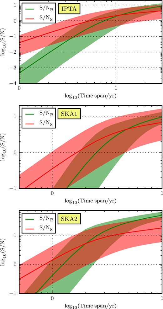
Although addressing when we will detect GWs with PTAs is not the main goal of this work, the first natural outcome of our calculation is the DP of each class of sources as a function of time: γB for a GWB, and γS for an individual source. This is presented in Fig. 2 for the three investigated arrays. In each panel, we show the result for a specific PTA, considering the whole signal and progressively subtracting the lowest frequency bins.
![DP (averaged over all realizations of the ensemble of SBHBs) versus observing time of a GWB (green lines) and a single source (red lines) assuming the IPTA (upper panel) SKA1 (middle panel) and SKA2 (lower panel). Solid lines show DPs integrated over all the frequency range [T−1, Δt−1], whereas the dashed (dotted) lines show the result when the lowest frequency bin (two lowest bins) are removed from the calculation.](https://oup.silverchair-cdn.com/oup/backfile/Content_public/Journal/mnras/451/3/10.1093/mnras/stv1098/2/m_stv1098fig2.jpeg?Expires=1750301495&Signature=elNPMN7kLr9Kxb97sdSDMmR8mogeigg4zi8L2ktW3LIPiv97870MmjCi6TEVzTogQFnzhGVBFRwbt2P~Ooqcdh8Q7EtcqfkZQRpiwKG-YFo6zyiDBWuVh92oc8FS926Smo3ZGV6sclGiOo~aShqfE2oa3rmByEIDT5gmUDt4ohwe8vdM~GxbHMlnvTD2ewn1i4l~fOIg9YdlefQxSl2L2XIOD7pYHFlq4jnyGUwhFDgR5JphRLjQLUILFd0Tqn-zj3QIgMq9C8nGYuCetJ9FXWGVNcDuOr1Pp3mEsqcGTuRneRBtZjfo0IMFSpuLlRNCsDjsfTIsJCIj5cvSPxeWkQ__&Key-Pair-Id=APKAIE5G5CRDK6RD3PGA)
DP (averaged over all realizations of the ensemble of SBHBs) versus observing time of a GWB (green lines) and a single source (red lines) assuming the IPTA (upper panel) SKA1 (middle panel) and SKA2 (lower panel). Solid lines show DPs integrated over all the frequency range [T−1, Δt−1], whereas the dashed (dotted) lines show the result when the lowest frequency bin (two lowest bins) are removed from the calculation.
It is clear from Fig. 2 that the subtraction of the lowest frequency bins has a larger impact on the DP of the GWB than on the DP of single sources. This is because there are more binaries emitting at lower frequencies, and thus the GWB becomes stronger, and more likely to be detected, at the lowest frequency bins. For single sources, the trend is different. On one hand, at very low frequencies there are more binaries, but they are hardly resolvable, i.e. the GWs produced by all other binaries act as a noise that masks the signal of an individual source. On the other hand, at high frequencies, although single sources are easier to resolve (since there are fewer binaries emitting at similar frequencies), it is less likely to find one emitting strong enough GWs to be detectable. There is thus a particular range of frequencies (not necessarily the lowest or the highest frequency bins) where single sources are more easily detectable.
The green curves in the upper plot of Fig. 2 show the predicted DP of a GWB for the IPTA. The current array has been running for ≈10 yr, which corresponds to a DP of ≈37 per cent assuming pure white noise (solid green curve). However, the DP at 10 yr goes down to ≈5 per cent and <1 per cent when the lowest and the two lowest frequency bins are taken out of the computation. Another way to put this is by looking at the 50 per cent DP: this probability is reached in approximately 2, 9, and 16 yr from now, depending on the cut-off on the low-frequency bins.
The DP for individual sources with the IPTA (red curves in the upper plot of Fig. 2) is, on the other hand, always relatively small, reaching values around 10–20 per cent after 20 yr from now. This should not be taken as an indication against the development of single source searches. First, we adopted a fairly conservative criterion for the detection of single sources, placing a threshold of FAP α = 0.1 per cent; it could be possible that the signal looked like a collection of relatively faint hotspots in the sky, not classified as single sources in our computation, but also not similar to a GWB. A search for multiple single sources (Babak & Sesana 2012) might be more efficient than a search for a GWB in such situation. Secondly, these predictions assume the current array without any future improvement. Adding more pulsars and, most importantly, reducing the rms of individual pulsars will result in a much higher chance of detecting a single source, which is what we expect as we enter the SKA era. Indeed, this is shown in the middle and lower panels of Fig. 2 (note that the x-axis now runs to 10 yr only). With the full SKA PTA (described in Section 2.4), the detection of a GWB will be almost certain within 5 yr, whereas single sources will be detected with a probability higher than 80 per cent after 10 yr. The higher probability of detecting individual sources stems from the lower rms expected from individual pulsars in the SKA era. The PTA will start to ‘hit the signal’ at much higher frequencies (f > 10−8 Hz), where it is also likely to see individual sources and not only an unresolved GWB. We notice, none the less, that these numbers are quite less optimistic that those quoted in Janssen et al. (2014). This is because, in that paper, both the GWB and single sources are said to be detectable if the produced S/N is larger than 4. However, it turns out that this is not sufficiently stringent for claiming a confident detection of a single source. One should consider the results of this work as an update to those claimed in Janssen et al. (2014), keeping in mind some important caveats related to the possible resolution of multiple sources that we will discuss in Section 4.
Let us stress once again that when calculating the DP for the SKA, we neglect previous IPTA data. One could achieve a more accurate prediction by adding millisecond pulsars to the IPTA gradually, until reaching the SKA1 configuration. This may be considered for a future work, whereas in this paper we attempt to focus on the detection capabilities of the current IPTA, and compare it with a PTA constructed with the SKA.
3.2 Signal-to-noise ratio
As explained in Section 2, the probability of detecting a GW signal is evaluated in this paper using the DP instead of the S/N, which is more commonly used in the related literature. We now explore the properties of the S/N of the two types of signals.
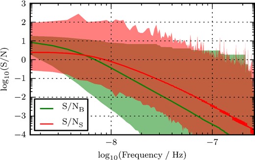
S/NS and |${\rm S/N}_{\rm B}^{f_i}$| versus observed GW frequency. The red area contains the S/NS values of the strongest binaries in each frequency bin, for all of our realizations of the SBHB population; the red line gives the average S/NS over all realizations. The green area contains the cumulative contributions to S/NB above each particular frequency bin, |${\rm S/N}_{\rm B}^{f_i}$|, defined in equation (48); the green line gives the mean |${\rm S/N}_{\rm B}^{f_i}$| at each bin. Thus, the left-most point of the green line gives the ensemble average S/NB.
The evolution of the S/N as a function of the observation time is shown in Fig. 4, for IPTA, SKA1, and SKA2. The S/N presents similar features for both classes of sources, behaving as a double power law; however, their detailed evolution is different, and the two curves end-up intersecting at some point. The S/N produced by a GWB follows the trend already predicted by Siemens et al. (2013), which is not surprising, given that the formula they use to calculate the S/N is almost identical to ours (numerically, the difference is negligible), in equation (A19). One thing that is worth noticing is that the specific value at which the S/N flattens out for long observing times does only depend on the number of pulsars in the array. In the IPTA case, where 15 pulsars give a major contribution to the detection statistic (having a rms noise which is eight times better than the others) the turnover starts already at S/N ≈1, whereas in the SKA2 case, where 200 pulsars equally contribute to the array, the turnover starts only at S/N ≈10. In practice, we have a turnover by S/N ∝ M1/2, where M is the number of pulsars. Therefore, having an array formed by many pulsars with decent precision might be a better strategy to detect a GWB than having few ultraprecise pulsars (a point that has also been made by Siemens et al. 2013).
S/N versus observation time, for an IPTA (top), SKA1 (central), and SKA2 (bottom). The red area covers the values between the 5th and 95th percentiles of S/NS of all realizations; the red line is the average over realizations. The green area covers values between the 5th and 95th percentiles of S/NB, and the green line is the average.
The S/N of single sources grows initially faster than quadratically in time, because by accessing lower and lower frequencies (but still higher than 10−8 Hz, where SBHBs are still quite sparse) there is a larger chance to detect a new bright individual source. However, after enough observation time, when frequencies lower than 10−8 Hz start to be accessible, individual sources with high S/N become less likely to be found. At that stage, the S/N of an individual source grows as T1/2, as suggested by equation (36).
By inspecting the upper plot in Fig. 4, one could claim that the detection of a single binary is currently (by ≈10 yr of observing time span for the IPTA) more likely than that of a background, since the average S/NS is larger than S/NB. Moreover, if one assumes that a detection is achieved as soon as the S/N surpasses a certain threshold (for example 4, as in Janssen et al. 2014), one would also claim that detecting a single SBHB is more likely than detecting a GWB for the two SKA configurations considered. However, both claims would be wrong; as we mentioned in Section 2, the detectability should be evaluated in terms of the DP, and, as shown in Fig. 2, the probability of detecting a GWB is in all cases (for all PTAs and observing times considered) larger than that of detecting a single SBHB.
3.3 What will be detected first?
We compute PS(T) as a function of the observation time T for the different arrays considered in this work; the result is shown in Fig. 5. There we see that, if the IPTA array keeps going for other 20 yr, there is only about a 4–8 per cent probability that the first claimed detection is of a single source. Thus, the first detected PTA signal will most likely be a GWB or an incoherent superposition of multiple sources. Things will change significantly (but not dramatically) in the SKA era. An SKA1-type PTA will have a 8–13 per cent chance to detect a single source first, a percentage that might increase to about 12–25 per cent in the SKA2 phase. Note that the aforementioned probabilities depend on the treatment of the lowest frequency bin. In particular, when all low-frequency bins are considered, the DP of the GWB becomes much larger than that of single sources, and hence the probability of detecting a single source before a GWB becomes lower and saturates earlier (solid curves in Fig. 5). To be conservative, we assume that the lowest frequency bin has a smaller contribution in the signal build-up, because of the timing model fitting; then, omitting the results in which all frequency bins are considered, we can confidently say that the chance to detect a single source before a GWB lies between 7 and 25 per cent, depending on the array configuration.
![Cumulative probability of detecting a single resolvable source before a GWB versus observing time, for the IPTA (top panel), SKA1 (central panel) and SKA2 (bottom panel). In each panel, solid lines show DPs integrated over all the frequency range [T−1, Δt−1], whereas the dashed (dotted) lines show the result when the lowest bin (two lowest bins) are removed from the calculation.](https://oup.silverchair-cdn.com/oup/backfile/Content_public/Journal/mnras/451/3/10.1093/mnras/stv1098/2/m_stv1098fig5.jpeg?Expires=1750301495&Signature=Ry4UClRW4oUwcsYzOxfpBV-G3bA~7zxXANObhugK5YKB0VEugJxykVt-8ciFN22L8~e1LsJOmfWURJrk0Ta~NPiI1iFdIixT9IauraSUZxGPByS6sR62Lypp~UtqaZj753Z6B05hzlC8SpVZyk79yEYL1EtGdJ4kvCQsZ2AcU4IFA4qmw8fG~TV6eSp4uRwr5WNncQA0yHiE0vDEylvmdE~A1035503wAh8veZRabp71E96crZkHvRsQ4fSYXHoCpoPi80Tk1gLuJQy-MuewDm3tZZvarBMXYynczHX03WhtXDtnTHHl34a1MH233II95MJpG4qfyDVhfEoXb9-PFA__&Key-Pair-Id=APKAIE5G5CRDK6RD3PGA)
Cumulative probability of detecting a single resolvable source before a GWB versus observing time, for the IPTA (top panel), SKA1 (central panel) and SKA2 (bottom panel). In each panel, solid lines show DPs integrated over all the frequency range [T−1, Δt−1], whereas the dashed (dotted) lines show the result when the lowest bin (two lowest bins) are removed from the calculation.
3.4 Properties of the first detectable single source
Even though single sources will most likely be detected after a GWB, they will eventually pop-up in PTA data. It is therefore interesting to study their properties in terms of mass, redshift and GW frequency. We summarize this information in Fig. 6 for all the investigated arrays and different observation times. All frequency bins were taken into account when constructing this figure (even the lowest ones). To construct these distributions, we took all the realizations of the SBHB population and considered, at any observation time, the brightest source in each frequency bin, weighting their contribution by their DP.
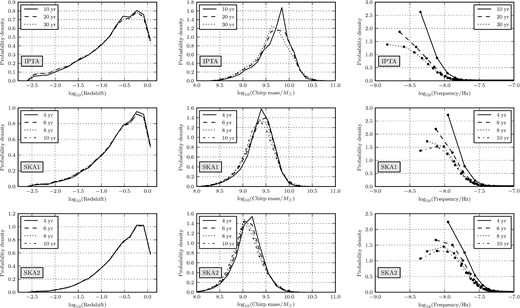
Properties of the individual SBHBs that are most likely to be detected with the current IPTA (upper row plots), SKA1 (central row) and SKA2 (lower row). The different columns of plots show, from left to right, the PDF of redshift, chirp mass, and GW observed frequency of the individual SBHBs. The black points in the graphs on the right-hand column are located at the arithmetic mean of the frequency bins.
The properties of the first detectable single sources do not depend strongly on the assumed PTA. The vast majority of the sources are massive, nearby binaries, clustering in the redshift range 0.3–0.7, regardless of the PTA properties. In terms of chirp mass, the more sensitive the array, the less massive the first detectable binaries would be. Therefore, although the IPTA has a chance to detect binaries with |${\cal M}>10^{9.5}\,\mathrm{M}_{\odot }$|, SKA2 will observe many more systems with |${\cal M}\approx 10^{9}\,\mathrm{M}_{\odot }$|. The rms noise of the pulsars in the array also has an impact in the frequency distribution of the systems (right-hand panels). In a putative IPTA scenario, the higher DP is always at the lowest frequency, despite the fact that more sources contribute to the signal in that range, and the inherent probability of having a single source sticking out is smaller. This is simply because the individual pulsar rms in the IPTA is not good enough to allow efficient detection at high frequencies, and sources must be extremely bright to be observed there. Conversely, in both SKA scenarios (central and lower rows of plots), the single source DP peaks around 10−8Hz, even if the observation time is extended to 10 yr and lower frequencies are accessible. This is simply because the array sensitivity now allows the detection of individual sources also at higher frequencies, making clear that the presence of these systems becomes intrinsically less probable at progressively lower frequencies.
3.5 Pulsar term of the first single source
The GWs arriving at our galaxy produce a deformation of the space–time metric that can be observed in two ways: via the Earth term and via pulsar terms. The Earth term affects the ToAs of the pulses of all pulsars at the moment when the GWs reach Earth. On the other hand, a pulsar term is originated when the GWs reach any of the pulsars; the distorted pulses emitted by that pulsar are observed by our telescopes after they travel all the way from the pulsar to Earth. Thus, there is a delay between the Earth term and any observable pulsar term, of hundreds or thousands of years, depending on the distance to the pulsar and its relative angle with respect to the GW source. Consequently, it is possible to observe GWs of a single source at two different stages of the binary's lifetime, differing hundreds or thousands of years. The question we address now is, does the GW frequency differ significantly between the Earth and pulsar terms? This is an interesting topic that has consequences in the development of data analysis algorithms targeting continuous GW sources.
The most distant pulsar in the current IPTA is at ∼6 kpc. The maximum delay between pulsar and Earth terms for this pulsar would be of ∼12 kpc c−1, which is twice the light travel time between that pulsar and Earth. This delay would be achieved if the SBHB was located exactly at the opposite sky location of the pulsar. We calculate f P of all binaries in each realization of the Universe, assuming |$\Delta \mathcal {T}=12\,$|kpc c−1, and also |$\Delta \mathcal {T}=3\,$|kpc c−1, which would be a typical delay for average IPTA pulsars (the mean estimated distance to IPTA pulsars is ≈1.5). Then we obtain the frequency shift between the pulsar and the Earth term, [f E − f P]/Δf, where Δf = T−1, and T is the observing time needed to detect the SBHB.
The distribution of frequency shifts of the first detectable binary for all the considered PTAs is shown in Fig. 7, assuming |$\Delta \mathcal {T}=3\,$|kpc c−1 (upper plot) and |$\Delta \mathcal {T}=12\,$|kpc c−1 (lower plot). All histograms are weighted by the DP of the binaries, so that binaries with larger probability of being detected are more representative than those with smaller DP. By looking at the figure, one can conclude that a significant evolution between pulsar and Earth term is not likely; among binaries detected in the near future with the IPTA, a shift of at least 1 bin has a probability of 22 per cent for average pulsars (at around 1.5 kpc), and to 33 per cent for a pulsar at 6 kpc. These percentages increase as we move into the SKA era; for an SKA2 arrays the odds of having a sizeable frequency shift between the pulsar and the Earth terms become higher than 50 per cent, due to the fact that single sources are detected at higher frequencies, where their chirping becomes progressively faster. All in all, we can conclude that frequency-shifting and strictly monochromatic individual sources are roughly equally likely to be detected.
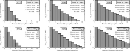
Histogram of the frequency shift between the pulsar and Earth terms, in units of the frequency bin T−1), where T is the observing time (assumed 10 yr in all cases), for the current IPTA (left-hand panels), SKA1 (central panels) and SKA2 (right-hand panels). The upper plots assume a typical observed time delay consistent with the mean estimated pulsar distance in the current IPTA (≈1.5 kpc). The lower plot assumes a typical time delay consistent with the maximum pulsar distance in the current IPTA (≈6 kpc).
4 DISCUSSION AND CONCLUSIONS
The results shown in the previous section have a number of important implications for the future design of PTA observations and data analysis pipelines.
We showed that a GWB is more likely to be detected than any resolvable single source, which is consistent with other recent predictions (Rosado & Sesana 2014; Ravi et al. 2015). However, this result should not discourage the development of single source detection pipelines for at least two reasons. First, there is a 5–25 per cent probability of detecting a single source first, which is not negligible; in particular, if the IPTA sensitivity will prove insufficient, expected timing improvement in the SKA era will result in an increase of the odds of detecting a single source. Secondly, throughout the paper we adopted a conservative definition of GWB (isotropic, stochastic, Gaussian, unpolarized, and stationary); the true signal produced by the superposition of GWs coming from the ensemble of SBHBs might well be dominated by a handful of signals, therefore significantly departing from isotropy and/or Gaussianity. The development of detection algorithms targeting multiple individual sources (Babak & Sesana 2012; Petiteau et al. 2013) as well as certain types of anisotropic signals (Gair et al. 2014) might prove to be a ‘more optimal’ strategy than searching for a GWB with the aforementioned properties.
Predictions should generally be reported in terms of DP and not S/N. From a frequentist perspective, what matters is the DP at a fixed FAP; a concept which translates into different S/N values for different types of sources and different data analysis techniques. In our specific case, for fixed DP and FAP, a much larger S/N is required for the detection of a single source than for the detection of a GWB, because of the large number of templates needed in the search of the former. Moreover, even within the same class of sources, depending on the adopted statistic, fixing DP and FAP may result in a time-dependent S/N threshold (in particular when the GWB becomes no longer a weak signal), which is the case for both our A- and B-statistics,6 as discussed in Section 2.2.
None the less, the S/N behaviour as a function of time encodes interesting information about source detectability. Both the S/N of a GWB and of a single source increase rapidly with time in the weak signal limit, but after the weak signal regime is abandoned the increase becomes slower. The transition between the two regimes appears to happen at an S/N ∝ M1/2, as shown in Fig. 3. Therefore, adding to a PTA many pulsars with decent precision might be a better strategy to detect any type of signal than having few ultraprecise pulsars (a point that has also been made by Siemens et al. 2013, in the GWB case), and this issue is certainly worthy of further investigation.
The first single sources to be detected will likely be extremely massive (|$\mathcal {M}>10^9\,\mathrm{M}_{\odot }$|), and emitting at a GW frequency of ≈10 nHz. Incidentally, for typical millisecond pulsar distances of ∼kpc, the transition between evolving/non-evolving sources occurs at about that same frequency. Therefore, it is impossible to discard a priori waveform models and/or detection techniques. For example, from a frequentist perspective, both |${\cal F}_p$| and |${\cal F}_e$| statistics are equally important tools, and no option should be discarded.
Those results were obtained under a number of simplifying assumption that we now discuss.
We assumed circular, GW-driven binaries. Although this assumption might be reasonable, SBHBs observable with PTAs, are at the centi-to-milliparsec separations, where the coupling to the environment can still play a role. This fact has been pointed out by a number of authors (Kocsis & Sesana 2011; Sesana 2013a; McWilliams et al. 2014; Ravi et al. 2014), and might be relevant for the results reported above. Efficient environmental coupling drives SBHBs faster towards coalescence; the net effect is that there are less systems contributing at each frequency bin, and the odds that a single source will dominate the signal are likely to increase. We therefore speculate that environmental coupling, although damaging in terms of GWB detection, might promote the detection of single sources. On the other hand, environmental coupling might also result in very eccentric binaries (Sesana 2010; Roedig & Sesana 2012). In this case, each individual system will emit in a whole range of GW harmonics, resulting in a more complicated signal. The development of data analysis pipelines for eccentric SBHBs has recently begun (Zhu et al. 2015), but the DP of such systems requires further investigation. Regardless of the precise mechanism that could affect the actual shape of the GWB, their overall effect could be a lower amplitude of the signal around the lowest frequency bins. Thus, in practice, subtracting the contribution from the lowest frequency bins (which we did in previous sections in order to simulate the effect of the timing model) could be a sensible way to mimic the reduction in the signal. In such a case, the DP, plotted in Fig. 2, would be well modelled by the dashed and dotted curves, that disregard the signal from the lowest and two lowest bins, respectively.
When evaluating the DP of single sources, we considered only the loudest binary at each frequency bin, and treated the rest of the signal as a stochastic GWB. However, such approximation might be too crude, since the rest of the signal might be dominated by just a few SBHBs. Babak & Sesana (2012) showed that an array of M equally good pulsars can in principle resolve M/3 sources at each frequency. Although the IPTA data set is dominated by a few, very good pulsars, and the resolution of multiple sources seems unlikely, things will be different in the SKA era. Having a large number of extremely stable pulsars might realistically favour the resolution of multiple SBHBs at each frequency, and, in this respect, the 80 per cent DP probability for singles sources with an SKA2-type array should be regarded as a robust lower limit.
When calculating the detectability of a single source, the sky location of the SBHBs is taken into account; one can see this in equation (46), that depends on the sky coordinates of the binary and the pulsar. However, the DP of a GWB is insensitive to the particular distribution of the binaries over the sky; the function Sh, that encompasses the information about the signal in the DP, depends on the characteristic amplitude of the GWB, made up as the superposition of the GW strains from all SBHBs in the ensemble (summed in quadrature). This implies that the particular location of the binaries on the celestial sphere is not relevant (only the distance to the binaries is), and the contribution of the ensemble to the cross-correlation is equivalent to that of an isotropic GWB. In other words, the signal of each binary is isotropically smeared out over the sky. This can favour the predicted detectability of a GWB over single sources,7 since the statistic employed for the detection of the background is optimal for an isotropic signal. If the ensemble of SBHBs produced a rather anisotropic signal, it could still be detected with a cross-correlation analysis, but the result would be suboptimal (Cornish & Sesana 2013). In such a case, a search for an anisotropic GWB (Mingarelli et al. 2013) or a search for multiple sources (Babak & Sesana 2012) would be more efficient, although the performance of an isotropic search or an optimal anisotropic search when the background is anisotropic is likely to be a bit lower than that of an optimal isotropic search for an isotropic background, which could delay detection. A more sophisticated way to evaluate the detectability of the GWB would require the DP to be sensitive to the sky distribution of binaries, by considering the contribution of each binary to the residuals of each pulsar in the array. Given the large amount of simulations analysed in this work, such a task would presumably become computationally involved. We point out, none the less, that the DP of the GWB has most of its contribution from the lowest frequency bins, where the background in most models can safely be considered isotropic. Significant anisotropies, that arise when the background is dominated by fewer binaries, are usually important at rather high frequencies, that do not contribute as much to the DP. Therefore, we expect that this possible overestimate of the GWB DP should not be significant, and evaluating the detectability of the GWB with a more sophisticated approach would not change the conclusions of this work.
We considered ideal millisecond pulsars described by white noise only, ignoring the impact of fitting for a timing model. This issue was already commented on in previous sections, as well as the possibility of including unmodelled red noise in our estimates. We defer a more comprehensive treatment of the pulsar noise model to a future work.
We considered very idealized PTAs, assuming that the IPTA will simply continue as it is now, without adding any further pulsar, or improving their timing precision. Moreover, we kept IPTA and SKA separated; a realistic computation of PTA DPs in the SKA era should take into account all previous, valuable IPTA data.
Despite all these limitations and caveats, the calculation we presented here is the first quantitative attempt at assessing the ‘single versus background’ issue. An unresolved GWB is more likely to be detected, but there is a sizeable chance to see a single source first, and the development of the relevant detection pipelines should not be stopped. An extension of this work to more realistic PTAs and source populations including environmental coupling and eccentricity will be crucial to direct the development of data analysis pipelines and to possibly bring the first GW detection with PTAs closer in time.
ACKNOWLEDGEMENTS
The authors thank the useful help and comments from Bruce Allen, Carsten Aulbert, Stas Babak, Ewan Barr, Neil Cornish, Justin Ellis, Ilya Mandel, Giulio Mazzolo, Antoine Petiteau, Joe Romano, Stephen Taylor, Yan Wang, Karl Wette, and Xingjiang Zhu. AS and JG are supported by the Royal Society through the University Research Fellow scheme.
Throughout this section, by ‘realizations’ we do not refer to the outputs of the computer simulations analysed in other sections of this paper, but to a hypothetical set of copies of the same Universe.
We assume that the optimal way to cross-correlate many detectors is to combine them in pairs (Allen & Romano 1999).
This amounts to simply add an appropriate Sj, red to the noise power spectrum of each pulsar, yielding |$P_j=2\sigma _i^2\Delta t+S_{j,{\rm red}}$|.
We note that this does not apply to the statistic employed by Siemens et al. (2013), which is similar to our B-statistic, but with a subtle difference in the definition of the null hypothesis: they assume that all pulsars show a common but uncorrelated red noise (due to some unknown physical process) whose spectral shape mimics exactly that of the GWB. Under this conservative assumption, σ0 = σ1, and the S/N threshold corresponding to a given DR at a fixed FAP is indeed constant in time. A more detailed study of the statistic used in Siemens et al. (2013) can be found in Chamberlin et al. (2015).
We thank Neil Cornish for pointing out this possible caveat.
REFERENCES
APPENDIX A: OPTIMAL STATISTICS FOR GWB DETECTION
A1 Cross-correlation
The true optimal statistic will be the combination that maximizes the DP at a fixed FAP, but as a proxy for this it is usual to consider statistics that maximize the S/N, which is the ratio of the expected value of a statistic in the presence of a signal, μ1, to its standard deviation. The standard deviation can either be computed in the absence of a signal, σ0, or in the presence of a signal, σ1. The A-statistic was constructed to maximize μ1/σ0. This can be thought of as a measure of the significance level at which a given source has a good chance of being detected. The noise-only standard deviation σ0 determines the FAP, and a given FAP therefore corresponds to a certain number of standard deviations, kσ0. Assuming a symmetric distribution, a source with μ1/σ0 = k has a 50 per cent chance of being detected if the threshold is set to that FAP. The B-statistic was constructed to maximize μ1/σ1. This is a measure of how inconsistent such a signal is with noise. The posterior distribution in the presence of a signal will have width σ1 and so this statistic measures the number of standard deviations above 0 the mean of the posterior lies. As we will see below, the two statistics are equivalent in the weak-signal regime, but the B-statistic is more robust for stronger GWBs.
A2 A-statistic
A3 B-statistic
A4 Comparison
We finish with three comments.
First, the function Sh0 appearing in these statistics is not known a priori. In practice, this quantity is what we are trying to measure with our observations. In the case of PTAs, it is most likely that the background will come from a population of merging SBHBs of the type described in this paper and for which the slope should be very close to Sh ∝ f−13/3 and so fixing this as the frequency dependence of Sh0 is likely to be close to optimal. The amplitude is not known a priori and does not cancel out of the expressions for the B-statistic. One reasonable strategy would be to compute the amplitude of a marginally detectable background, i.e. fix the FAP and compute the background amplitude that yields a ∼50 per cent probability of detection, and use this in Sh0. Again this should be near optimal when a background is first detected and will still yield confident detections for louder backgrounds, even though it will be suboptimal at such amplitudes. Other approaches, such as using a set of statistics constructed with a range of different functions Sh0, or an iterative approach in which an estimate of the amplitude obtained from the measured data is used to contract a new statistic and so on, would also be possible. An investigation of these approaches to data analysis is beyond the scope of this paper. However, we found that, in practice, the performance of the statistic did not depend strongly on the assumption about Sh0 and so for all the calculations in this paper we assume perfect knowledge of the background and set Sh0 = Sh.
Secondly, in deriving the B-statistic we ignored the off-diagonal elements of the cross-correlation matrix. The B-statistic will be valid in an intermediate signal regime, but will become suboptimal at large background amplitudes due to the omission of these terms. This was also discussed in Allen & Romano (1999), where it was argued that these terms were always subdominant for observations with GBDs. The importance of these terms has not been investigated for PTAs.
Finally, neither the A-statistic nor the B-statistic is truly optimal in the sense of maximizing the DP for a fixed FAP. Not only have off-diagonal correlations been ignored in deriving the B-statistic, but the procedure of maximizing μ1/σ0 or μ1/σ1 is not equivalent to maximizing the DP. Under a Gaussian assumption we need to maximize [μ1 − kσ0]/σ1, where k is a constant that depends on the chosen FAP. This maximization can be done, although it is more difficult, and we did not consider it here. Simulations indicate that both the A- and B-statistics are nearly optimal in the weak signal limit, while the B-statistic continues to be near optimal for higher background amplitudes.
