


Abstract
Radio relics in galaxy clusters are associated with powerful shocks that (re)accelerate relativistic electrons. It is widely believed that the acceleration proceeds via diffusive shock acceleration. In the framework of thermal leakage, the ratio of the energy in relativistic electrons to the energy in relativistic protons should be smaller than Ke/p ∼ 10−2. The relativistic protons interact with the thermal gas to produce γ-rays in hadronic interactions. Combining observations of radio relics with upper limits from γ-ray observatories can constrain the ratio Ke/p. In this work, we selected 10 galaxy clusters that contain double radio relics, and derive new upper limits from the stacking of γ-ray observations by Fermi. We modelled the propagation of shocks using a semi-analytical model, where we assumed a simple geometry for shocks and that cosmic ray protons are trapped in the intracluster medium. Our analysis shows that diffusive shock acceleration has difficulties in matching simultaneously the observed radio emission and the constraints imposed by Fermi, unless the magnetic field in relics is unrealistically large ( ≫ 10 μG). In all investigated cases (also including realistic variations of our basic model and the effect of re-acceleration), the mean emission of the sample is of the order of the stacking limit by Fermi, or larger. These findings put tension on the commonly adopted model for the powering of radio relics, and imply that the relative acceleration efficiency of electrons and protons is at odds with predictions of diffusive shock acceleration, requiring Ke/p ≥ 10 − 10−2.
1 INTRODUCTION
Radio relics are steep-spectrum radio sources that are usually detected in the outer parts of galaxy clusters, at distances of ∼0.5–3 Mpc from their centres. They are very often found in clusters with a perturbed dynamical state. There is good evidence for their association with powerful merger shocks, as earlier suggested by Ensslin et al. (1998). Among them are giant double-relics that show two large sources on opposite sides of the host cluster's centre (e.g. Bonafede et al. 2012; Feretti et al. 2012; de Gasperin et al. 2014). These relics are associated with shocks in the intracluster medium (ICM) that occur in the course of cluster mergers. Only a tiny fraction of the kinetic power dissipated by typical cluster merger shocks (≪10−3) is necessary to power the relics, and diffusive shock acceleration (DSA; Caprioli e.g. 2012; Kang & Ryu e.g. 2013, for modern reviews) has so far been singled out as the most likely mechanism to produce the relativistic electrons and to produce the observed power-law radio spectra (e.g. Hoeft & Brüggen 2007). However, if the standard DSA model is correct, the same process should also lead to the acceleration of cosmic ray (CR) protons. Indeed, the process should be much more efficient for protons, owing to their larger Larmor radius.1
To date, high-energy observations of nearby galaxy clusters have not revealed any diffuse γ-ray emission resulting from the interaction between relativistic protons and thermal particles of the ICM (Reimer et al. 2003; Aharonian et al. 2009; Aleksić et al. 2010, 2012; Arlen et al. 2012; Zandanel & Ando 2014). Recently, the non-detection of diffuse γ-ray emission from clusters by Fermi has put the lowest upper limits on the density of CRs in the ICM, ≤ a few per cent of the thermal gas energy within the clusters virial radius (Ackermann et al. 2010, 2014). Moreover, the stacking of subsets of cluster observations leads to even lower upper-limits (Huber et al. 2013; Griffin, Dai & Kochanek 2014). These low limits on the energy content of CRs can be used to constrain shock-acceleration models. Recently, Vazza & Brüggen (2014) have already suggested that the present statistics of radio observations, combined with available upper limits by Fermi places constraints on DSA as the source of giant radio relics. In Vazza & Brüggen (2014), we assumed that the population of clusters with radio relics was similar to the population of NCC (non-cool-core) clusters for which the stacking of Fermi clusters was available. In this paper, we repeat a similar analysis by comparing to a more realistic stacking of the Fermi data. Our method is outlined in Section 2.1, while our results are given in Section 3. In the latter section, we also discuss on the role played by the several open parameters in our modelling. We find (Section 3) that the present upper limits from Fermi imply energy densities of CR-protons that are too low to be explained by standard DSA: if DSA produces the electrons in relics, then we should have already detected hadronic γ-ray emission in some clusters, or in stacked samples. In our conclusions (Section 4), we discuss possible solutions to this problem, as suggested by recent hybrid and particle-in-cell (PIC) simulations of weak, collisionless shocks.
2 METHODS
2.1 Semi-analytical cluster mergers
Our aim is to test DSA by making quantitative predictions of the hadronic γ-ray flux assuming that the CR-protons come from the same shocks that produce radio relics (Section 2.2.1). Semi-analytical methods with initial conditions tuned to match observable parameters of radio haloes have been widely used in the literature (e.g. Gabici & Blasi 2003; Cassano & Brunetti 2005; Hoeft & Brüggen 2007). They have obvious limitations owing to the lack of three-dimensional detail and the crude geometrical assumption on the merger scenario (i.e. spherical symmetry and simple radial distribution for the gas). Still, for this specific problem they are helpful, as the energy density of CR-protons should be a simple function of the shock parameters and of the volume crossed by each shock wave.
Our approach is similar to the method used in Vazza & Brüggen (2014): for each cluster in our sample, we model the shock trajectories and the associated CR-acceleration. We use simple 1D models of shock propagation in stratified atmospheres and use observables from radio and X-ray data, such as the spectral index, the distance from the centre, the radio power and the largest linear scale of each relic Bonafede et al. (2012, see also de Gasperin et al. 2014). Below we summarize the most important steps from Vazza & Brüggen (2014, see also Fig. 1), while in Section 3.2 we discuss the most relevant uncertainties in our model and assess their impact on our results.
We infer the Mach number, M, from the spectral index of the radio spectrum, s, at the injection region via |$M= \sqrt{}\frac{\delta +2}{\delta -2}$| (δ is the slope of the particle energy spectra and δ = 2 s). This assumes that the radio spectrum is dominated by the freshly injected CR-electrons at the shock, an assumption that might be poor for spectra integrated over large downstream volumes (in which cases the radio spectrum is steeper by 0.5). Bootstrapping with random deviates from the Mach number thus determined can quantify the errors (see Section 3).
The upstream (i.e. pre-shock) gas density, nu, at the relic is computed using a β-model profile for each host cluster, with β = 0.75 and the core radii scaling as rc = rc, Coma(TComa/T)1/2 (which follows from the self-similar scaling), where rc, Coma = 290 kpc. This is the only way to regularize our data set, as a more detailed reconstruction of the gas density from the literature is missing for most of these objects. Both are clearly a simplification but in reality we probably find higher gas densities and temperatures along the merger axis, due to clumping and enhanced gas compression which will only increase the γ-ray emission. Moreover, the propagation of each merger shock is determined by the temperature in front of it, i.e. in the upstream region, which present X-ray observation can hardly constrain for any of these objects. Therefore we always consider an upstream gas temperature, Tu, based on the LX–T500 relation for each host cluster (Pratt et al. 2009).
We compute the kinetic power for each shock as |$\Phi _{\rm kin}=n_{\rm u} v_{\rm s}^3 S/2$|, where vs = Mcs (|$c_{\rm s} \propto \sqrt{T_{\rm u}}$|).
We assume that a fraction of the kinetic power goes into CR-protons ΦCRp = η(M)Φkin, where the efficiency, η(M), is a non-linear function of the Mach number. It has been derived for several DSA scenarios (e.g. Kang & Jones 2007; Kang & Ryu 2013; Hong et al. 2014). Here, we use η(M) given by Kang & Ryu (2013), which were estimated based on simulations of non-linear DSA, considering an upstream β = 100 plasma and including a phenomenological model for the magnetic field amplification and Alfvenic drift in the shock precursor, due to accelerated CRs. This function predicts an acceleration efficiency of ≈1 per cent for M = 3, steeply rising to ∼10 per cent for M = 5 (see fig. 4 of Kang & Ryu 2013). The corresponding power into CR-electrons is set by assuming a fixed electron-to-proton ratio, Ke/p = 0.01: ΦCRe = Ke/pη(M)Φkin. This ratio is already conservative, as recent models of particle acceleration in supernovae suggest an even lower value, Ke/p ∼ 10−3 (Park, Caprioli & Spitkovsky 2015), which would result into a 10 times larger hadronic γ-ray flux than for our value of Ke/p.
- The magnetic field at the relic, B, is derived from the radio power via the equations given by Hoeft & Brüggen (2007). In this model the monochromatic radio power at frequency ν, Pν, depends on the shock surface area, S (which we derive from the projected size of the relic, assuming that the relic has a circular shape), the upstream electron density, ne (computed from nu by assuming a mean molecular mass of 0.6), the upstream electron temperature, Te ≈ Tu, the spectral index of the radio emission, s, and the relic magnetic field, Brelic, in the following way:where BCMB is the equivalent field of the cosmic microwave background.2 In our simplest model (‘basic model’), we let the magnetic field as a free parameter without upper limits, while in a more realistic scenario (‘Bcap’ scenario), we imposed a maximum magnetic field of Brelic, max = 10 μG for all relics (Section 3.2.1).(1)\begin{eqnarray} \frac{\mathrm{d}P}{\mathrm{d}\nu }&=&\frac{6.4 \times 10^{34} \,\rm erg}{\rm s \times Hz} \times S \times n_{\rm e} \times \eta (M) K_{\rm e/p} \frac{T_{\rm e}^{3/2}}{\nu ^{s/2}}\nonumber\\ &&\times \frac{B_{\rm relic}^{1+s/2}}{B_{\rm CMB}^2+B_{\rm relic}^2}, \end{eqnarray}
Explaining the observed radio emission from M ≤ 3 shocks is a problem, as the required electron acceleration efficiency at these weak shocks can become unrealistically large (Macario et al. 2011). It has been suggested that the contribution from shock re-accelerated electrons can alleviate this problem, as it would mimic the effect of having a higher acceleration efficiency (Kang, Ryu & Jones 2012; Pinzke, Oh & Pfrommer 2013). To model re-acceleration, as in Vazza & Brüggen (2014), we used an increased CR-proton acceleration efficiency as a function of Mach number, following Kang et al. (2007) and Kang & Ryu (2013) who showed that the net effect of re-accelerated and freshly injected CRs can be modelled by a rescaled efficiency η(M). This depends on the energy ratio between pre-existing cosmic rays (ECR) and the thermal gas (Eg). In the following, we parametrize this ratio using the parameter ϵ = ECR/Eg, and explore the cases ϵ = 0 (single injection, non-reaccelerated electrons), and bracket the trend of re-acceleration using ϵ = 0.01 and ϵ = 0.05. Note that the latest limits from Fermi only allows ϵ ≤ a few per cent, for flat radial distributions of CRs (Ackermann et al. 2014).
In order to compute the spectrum of electrons in the case of a re-accelerated pool of CRs, we follow Kang et al. (2012) and assume that the blend of several populations of pre-existing CR-electrons are characterized by a power law with index δe = (4δ + 1)/3, where δ is the spectral index of the energy spectrum derived at the relic as before. As in Kang et al. (2012), we fix the spectrum of re-accelerated CRs to the particle spectrum at the relic in those cases where the spectrum is flatter than the (steep) spectrum associated with the M = 2 shock that is supposed to re-accelerate them.
- Once the shock parameters are fixed, we estimate the energy injected in CR-protons that are assumed to stay where they have been predicted. We assume that each shock surface scales with the cluster-centric distance, r, as S(r) = S0(r/Rrelic)2 (i.e. the lateral extent of the shock surface is set to largest linear size of the relic, which decreases with ∝ r inwards). The cumulative energy dissipated into CR-protons is given byThe shock surface and strength will vary with radius, and so will the CR-proton acceleration efficiency, η(M). Our fiducial model assumes that the Mach number of shocks released by the merger is constant across the whole volume of interest, while in Section 3.2.3 we also test a scenario in which the Mach number scales with radius. The lower integration limit in the equation for ECR is the core radius, rc, meaning that the shocks are assumed to be launched only outside of the cluster core, which is supported by simulations (e.g. Vazza et al. 2012b; Skillman et al. 2013)(2)\begin{equation} E_{\rm CR}= \int _{r_{\rm c}}^{R_{\rm relic}}{\Phi _{\rm CRp}(r)v_{\rm s} \ {\rm d}r } = \int _{r_{\rm c}}^{R_{\rm relic}} \frac{\eta (M) n_{\rm u}(r) v_{\rm s}^3 S(r)}{2} \ {\rm d}r. \end{equation}
- We compute the hadronic γ-ray emission, Iγ, following (Pfrommer & Enßlin 2004; Donnert et al. 2010),with the only difference that for the hadronic cross-section we use the parametrization of the proton–proton cross-section given by Kelner, Aharonian & Bugayov (2006), as in Huber et al. (2013). In detail, we compute for each radius the source function of γ-rays as(3)\begin{eqnarray} q_{\gamma }(E_{\gamma })={{ 2^{4-\delta _{\gamma }} }\over { 3\delta _{\gamma }}} {{\sigma _{\mathrm{pp}}(E) c n_{\mathrm{e}}(r) K_{\rm p}}\over {\delta -1}} (E_{\mathrm{min}})^{-\delta } \frac{E_{\mathrm{min}}}{\mathrm{GeV}} \times \frac{m_{\pi ^{0}}c^{2}}{\mathrm{GeV}}, \end{eqnarray}where ne is the upstream electron density, computed from the gas density by assuming a molecular mean weight μ = 0.6. The spectrum of the γ-ray emission depends on the assumed Mach number across the cluster, and therefore is either a function of M(r) in the single acceleration model, or a constant in the re-acceleration case. Once the spectral index, δ, of the particle spectrum is fixed, the spectrum of the γ-ray emission is given by δγ = 4(δ − 1/2)/3 (Pfrommer & Enßlin 2004). Here, we consider hadronic emission in the energy range [0.2–300] GeV, which are compared to the stacked emission from Fermi described in the following section (Section 2.2.2). mπ and mp are the masses of the π0 and the proton, respectively. The threshold proton energy is taken as Emin = 780 MeV and the maximum is Emax = 105 MeV (the actual value is actually irrelevant, given the steep spectra of our objects) The effective cross-section we used iswith L = ln (E/1TeV) and |$E_{{\rm th}}=m_{\rm p}+2m_{\pi }+m^2_{\pi }/2m_{\rm p}\sim 1.22$| GeV (equation 79 of Kelner et al. 2006). The normalization factor Kp is(4)\begin{equation} \sigma _{{\rm pp}}(E)=(34.3+1.88L+0.25L^2)\left[1-\left(\frac{E_{{\rm th}}}{E}\right)^2\right]^4 \mbox{mb}, \end{equation}(5)\begin{equation} K_{\rm p}=\frac{(2-\delta )E_{\rm CR}(r)}{(E_{\rm max}^{-\delta +2}-E_{\rm min}^{-\delta +2})}. \end{equation}The emission per unit of volume, λγ, is obtained by integrating the source function over the energy range:where |$\mathcal {B}_{\mathrm{x}}(a,b)$| denotes the incomplete β-function and |$[f(x)]^{a}_{b} = f(a) - f(b)$|. Integrations over radii are performed by summing over radial shells of thickness 10 kpc. Finally, the hadronic γ-ray emission for each radial shell along the trajectory of the shock is given by λγ(r)S(r) dr and the total hadronic emission in the downstream region of each relic is given by the integral, |$I_{\rm \gamma }= \int _{r_{\rm c}}^{R_{\rm relic}} \lambda _{\gamma }(r) S(r) \ {\rm d}r$|.(6)\begin{eqnarray} \lambda _{\gamma }(r) &=& \int _{E_{1}}^{E_{2}} \mathrm{d}E_{\gamma } q_{\gamma }(E_{\gamma }) \nonumber \\ &=& \frac{\sigma _{\mathrm{pp}} m_{\pi }c^{3}}{3 \delta \delta _{\gamma }} \frac{n_{\mathrm{u}}(r) K_{\rm p}}{\delta -1} \frac{ (E_{\mathrm{min}})^{-\delta }}{2^{\delta _{\gamma }-1}} \frac{E_{\mathrm{min}}}{\mathrm{GeV}} \left( \frac{m_{\pi _{0}}c^{2}}{\mathrm{GeV}} \right)^{-\delta _{\gamma }} \nonumber \\ &&\times\, \left[\mathcal {B}_{\mathrm{x}}\left( \frac{\delta _{\gamma }+1}{2\delta _{\gamma }}, \frac{\delta _{\gamma }-1}{2 \delta _{\gamma }} \right) \right]^{x_{1}}_{x_{2}}, \end{eqnarray}
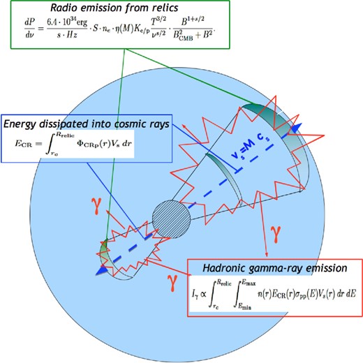
Schematic view of our method for computing γ-ray emission from accelerated CR-protons downstream of the double relics.
The above set of approximations minimizes the hadronic γ-ray emission from clusters: the presence of gas clumping and substructure is neglected, the injection of CRs is limited to regions outside of the dense cluster cores, and additional acceleration of CRs by earlier shocks, turbulence, supernovae and AGN is not taken into account. A number of assumptions have to be made in the previous steps. We discuss all most important in Section 3.2 and explore the effects uncertainties in the parameters of the model.
2.2 Observations
2.2.1 Radio data
We restrict our analysis of to double radio relics, as these systems are caused most clearly by major merger events (e.g. Roettiger, Stone & Burns 1999; van Weeren et al. 2011a; Skillman et al. 2013), and they should be less affected by projection effects because of large cluster-centric distances (Vazza et al. 2012b). We select double-relic sources from the collection of Bonafede et al. (2012) and further restrict analysis to the sources at high Galactic latitude (|b| > 15°) to avoid strong contamination by the bright diffuse γ-ray emission from the Galactic plane (see below). The final sample is made of 20 relics from 10 clusters: MACSJ1752, A3667, A3376, A1240, A2345, A3365, MACSJ1149, MACSJ1752, PLCKG287, ZwClJ2341 and RXCJ1314. The values of radio parameters for these objects (e.g. total power, radio spectral slope, s, largest linear scale of each object and distance from the centre of the host cluster) are given in Table 1.
Main observational parameters for the radio relics and clusters considered in this paper: redshift (second column), X-ray luminosity (third), distance from the cluster centre for each relic in the pair fourth and fifth column), largest linear scale (6 and 7), radio power (8 and 9), radio spectral index (10 and 11) of relics, upper limits of γ-ray emission at 0.2–300 and 1–300 GeV for each host cluster (12 and 13) and value of the test statistics (equation 7). The radio data are taken from Feretti et al. (2012) and Bonafede et al. (2012), while the γ-ray data have been derived from the Fermi catalogue in this work.
| Lx | r1 | r2 | R1 | R2 | log10(PR, 1) | log10(PR, 1) | |$\log _{\rm 10}(UL_{\rm 0.2{\rm -}300})$| | |$\log _{\rm 10}(UL_{\rm 1{\rm -}300}$|) | |||||
|---|---|---|---|---|---|---|---|---|---|---|---|---|---|
| Object | z | (1044 erg s−1) | (Mpc) | (Mpc) | (Mpc) | (Mpc) | (erg s−1) | (erg s−1) | s1 | s2 | [ph/(s cm2)] | [ph/(s cm2)] | TS |
| A3376 | 0.047 | 1.04 | 0.80 | 0.95 | 1.43 | 0.52 | 40.026 | 39.936 | 1.20 | 1.20 | −8.65 | −9.71 | 1.36 |
| A3365 | 0.093 | 0.41 | 0.56 | 0.23 | 1.00 | 0.70 | 40.086 | 39.146 | 1.55 | 1.93 | −8.61 | −9.66 | 6.17 |
| A1240 | 0.159 | 0.48 | 0.64 | 1.25 | 0.70 | 1.10 | 39.748 | 39.991 | 1.20 | 1.30 | −9.21 | −9.89 | 0 |
| A2345 | 0.176 | 2.56 | 1.50 | 1.15 | 0.89 | 1.00 | 40.544 | 40.577 | 1.30 | 1.50 | −8.55 | −9.55 | 6.19 |
| RXCJ1314 | 0.244 | 5.26 | 0.91 | 0.91 | 0.57 | 0.94 | 40.350 | 40.714 | 1.40 | 1.40 | −9.06 | −9.94 | 0 |
| MACSJ1149 | 0.540 | 6.75 | 0.82 | 0.76 | 1.39 | 1.14 | 40.879 | 41.100 | 1.20 | 1.42 | −9.53 | −10.11 | 0 |
| MACSJ1752 | 0.366 | 3.95 | 1.34 | 0.86 | 1.13 | 0.91 | 41.651 | 41.292 | 1.21 | 1.13 | −8.92 | −9.98 | 0.04 |
| A3667 | 0.046 | 1.02 | 1.42 | 1.83 | 1.30 | 1.30 | 40.044 | 39.945 | 1.39 | 1.31 | −8.59 | −9.64 | 3.16 |
| ZwCLJ2341 | 0.270 | 2.00 | 0.25 | 1.20 | 1.18 | 0.76 | 40.726 | 40.377 | 1.90 | 1.22 | −9.41 | −10.35 | 0 |
| PLCKG287 | 0.390 | 8.29 | 1.93 | 1.62 | 1.58 | 3.00 | 41.401 | 41.322 | 1.26 | 1.54 | −8.81 | −9.68 | 0.49 |
2.2.2 γ-ray data
We analysed γ-ray data collected by the Large Area Telescope (LAT) on board Fermi (hereafter Fermi-LAT). Fermi-LAT (Atwood et al. 2009) is a pair-conversion γ-ray telescope operating in the 20 MeV - 300 GeV band. We collected all the data obtained during the period 2008-08-04 to 2013-11-01 and analysed them using the fermi science tools software package v9r32p5 and the P7SOURCE_V6 instrument response files. For each source listed in Table 1, we extracted a rectangular region of interest (ROI) with side ∼20° × 20° centred on the source. For each source, we then constructed a model including the Galactic emission,3 the isotropic diffuse background4 and all sources listed in the 2FGL catalogue in a radius of 20° around our source, with spectral models and parameters fixed to the values given in 2FGL. We then performed a binned likelihood analysis (Mattox et al. 1996) on each individual ROI to determine the parameters of the γ-ray emission model. The normalization of each component (diffuse background components and point sources) was left free to vary during the fitting procedure.
In order to lower these limits, we performed a stacking analysis of the sources in our sample following the method presented in Huber et al. (2012, 2013). The stacking of the sources is performed by adding step by step the individual ROIs after having simulated and subtracted the surrounding point sources. The resulting co-added map for our stacked sample is given in Fig. 2. The co-added data are then fit using the same source+background model as described above. Again, no significant emission is measured within the stacked volume of these clusters (TSstacked = 0.21), which results in an upper limit of Fmean < 1.90 × 10⁻¹⁰ ph cm−2 s−1 (95 per cent CL, 0.2–300 GeV band) to the average flux per cluster. For more details on the stacking procedure and a thorough validation of the method using simulated data, we refer the reader to Huber et al. (2012).

Co-added Fermi-LAT count map in the 200 MeV–300 GeV energy range for all the clusters listed in Table 1. The circles indicate apertures of 2| $_{.}^{\circ}$|5 and 5° around the stacked cluster position to highlight the source and background regions, respectively.
3 RESULTS
3.1 Basic model
A typical set of predictions from our baseline model is given in Fig. 3 for the two relics in A3667. The integrated kinetic energy that crosses the shock (upper lines) and dissipated CR-proton energy (lower lines) in the second panel is integrated along the shock trajectory. In the single injection model (ϵ = 0), the predicted acceleration of CRs is very different for the two relics, and follows from the different assumed Mach numbers: M = 3.8 for the northern relic and M = 1.7 for the southern relic. In the first case, the radio power is matched with the modest field strength of Brelic ≈ 0.7 μG, while in the weaker southern shock the required magnetic field is ≈ 219 μG. Re-accelerated electrons can explain the observed radio power in both cases using fields in the range Brelic ∼ 1-2 μG. The γ-ray emission (lower panel) is the integrated hadronic emission in the downstream. Hence, the last bins on the left and on the right give the total emission from the two downstream regions and should be compared with the Fermi limit for A3667. When the contribution from both relics is summed up, the predicted hadronic emission is very close to the single-object limit from Fermi for this cluster. We find similar results for the relics in ZwCLJ2341 (see Table 2). In the next sections, we will discuss the predicted magnetic fields and the γ-ray emission from the full data set and under different assumptions in our model.
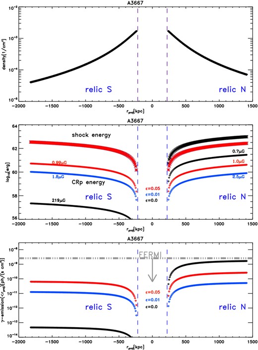
1D profiles of various quantities along the projected propagation radius of the two relics in A3667, as assumed or predicted by the basic model (Section 2.1). First panel: gas density profile. Second panel: profile of the cumulative shock energy and CRp-energy dissipated in the downstream. The additional numbers in colours give the magnetic field necessary to reproduce the observed radio power using equation (1). Third panel: predicted γ-ray emission. The vertical lines delimit the regions where the shocks have been launched, while the horizontal line gives the single-object limit from Fermi.
The full range of estimates from our fiducial model (Section 2.1) is shown in Fig. 4, where we plot: the distribution of predicted γ-ray emission for the full sample (histograms with different colours for each model) and compare the mean emission of each run (thin lines) with the limits we derive from our stacking of Fermi exposures on these objects (Section 2.2.2). This stacking gives us the most robust testing of DSA, since it comes from the same set of objects simulated with our semi-analytical method. In the same figure, we also show for completeness the result of stacking only NCC clusters in a larger sample of objects observed by Fermi (Huber et al. 2013), which we converted into the [0.2–300] GeV energy range by assuming a γ-ray spectral index of −2.6. The limit here is ∼5 times lower than our stacking limit (see also Griffin et al. 2014 for a slightly lower limit), given the larger sample of objects (32) and the fact that this sample contains more nearby objects than our list of radio relics. This limit comes from a bigger population, yet comparing it to our simulated population is useful, under the hypothesis that two parent population of objects are dynamically similar. This is likely, because to the best of our knowledge all objects of our sample are NCC and all show evidence of very perturbed dynamical states in X-ray (e.g. Edge et al. 2003; Cavagnolo et al. 2009; Bagchi et al. 2011; Bonafede et al. 2012, see also http://www.mergingclustercollaboration.org/merging-clusters.html). The magnetic fields at each relic required by our modelling of the radio power, using equation (1). We also show for comparison the upper limits derived on the magnetic field at the location of relics in the Coma cluster (Bonafede et al. 2013, based on the analysis of Faraday Rotation) and in the cluster CIZA 2242.2+5301 (van Weeren et al. 2010, based on the analysis of the brightness profile across the relic), as well as the range of values inferred by Finoguenov et al. (2010) for the relic north of A3667, based on the lack of Inverse Compton (IC) emission.
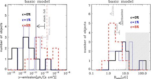
Left: distribution of predicted γ-ray emission from our cluster sample, for different fiducial models (coloured histograms). The thin vertical lines show the mean emission for the sample according to each model, and should be compared with the upper limits from the stacking of all NCC clusters observed by Fermi, or by the stacking limited to our sample of clusters with double relics (grey arrows). Right: distribution of magnetic fields (coloured histograms) required for each relic to match the observed radio power using equation (1). The additional grey arrows give the range of values inferred for the few observations of magnetic fields in real relics (see text for details), while the hatching marks the values of magnetic fields that we regard as physically unrealistic (see Section 3.2.1).
In our model, both ϵ = 0 and 5 per cent runs predict a very high mean level of hadronic emission, well above the stacking of this data set in the single injection case, and just below it in the case of ϵ = 5 per cent (but larger than the stacking of the full Fermi catalogue). In both cases, the mean emission is kept at a high value by 1/5 of bright objects in the sample (A3667 and ZwCLJ2341), however the bulk of all remaining objects is also characterized by emission of the order of the full stacking of NCC clusters. On the other hand, the ϵ = 1 per cent model predicts a mean emission below the stacking of this data set. However, the magnetic fields required in this case are very large. Here, six out of 20 relics require Brelic ≥ 10 μG where the radio emission is detected, which is at odds with the few available estimates of magnetic fields from observations (grey arrows). In a general sense, explaining fields larger than a few ∼ μG at the large radii where these relics are found is difficult based on both observational and theoretical facts (see Section 3.2.1 for a detailed discussion).
To summarize, none of the scenarios we investigated with our semi-analytical method is able to simultaneously predict a level of γ-ray emission compatible with Fermi and to use a reasonable magnetic field level in all objects. The re-acceleration model assuming 1 per cent of CR energy to be re-accelerated by merger shocks survives the comparison with Fermi, but makes use of very large magnetic fields in ∼1/3 of our objects. The models with single-injection or significant re-acceleration instead predict a mean emission for the sample which is in tension with stacking of Fermi observations for this sample, or for the larger sample of NCC clusters, which very likely has the same characteristics of the double-relics one.
The following sections will show how this problem is worsened as soon as all relevant assumptions made in our modelling are relaxed.
3.2 Model uncertainties
3.2.1 Magnetic field
First, we investigate the role played by the magnetic field in relics. Explaining magnetic fields larger than a few μG outside of cluster cores is very difficult for several reasons.
In the only case in which a good volume coverage of the ICM is obtained through Faraday Rotation (i.e. in the Coma cluster; Bonafede et al. 2010, 2013), the inferred trend of magnetic field is |$B \sim n^{-\alpha _{\rm B}}$|, with αB ∼ 0.5–0.9, which implies that on average the field drops below 1μG at half of the virial radius. This scaling is supported by simulations (Dolag, Bartelmann & Lesch 1999; Bonafede et al. 2010; Vazza et al. 2014b) and it implies that the magnetic field in the ICM is not dynamically important, i.e. βpl ∼ 100 everywhere (where βpl = nkBT/PB and PB is the magnetic pressure). Instead, a field of the order of ≥ 10μG at half of the virial radius or beyond implies β ≤ 1, which is hard to justify theoretically. Indeed, the turbulence around the relic should be modest and dominated by compressive modes, and can only raise the magnetic field by a small factor (Iapichino & Brüggen 2012; Skillman et al. 2013). It has been suggested that CRs can cause magnetic field amplification via CR-driven turbulent amplification (Brüggen 2013), but not to the extreme level required by our modelling. Moreover, all cosmological simulations predict some local amplification at shocks, but this is always smaller than the steep increase of the gas thermal pressure, due to Rankine–Hugoniot jump conditions (Dolag et al. 1999; Brüggen et al. 2005; Xu et al. 2009; Vazza et al. 2014b). Based on simulations, the observed mass–radio luminosity relation for double relics is better explained by assuming magnetic fields of the order of ∼ 2 μG in most objects (de Gasperin et al. 2014).
Evidence of polarized radio emissions from a few radio relics (including a few contained in our sample here) exclude the presence of large ≫ 10 μG fields distributed in scales below the radio beam (a few ∼ kpc), which would otherwise totally depolarize the emission (van Weeren et al. 2010; Bonafede et al. 2011, 2012). The highest (indirect) indication of magnetic fields in a giant radio relic so far is of the order of ∼ 7 μG (van Weeren et al. 2010). Moreover, all observations of Faraday Rotation outside of cluster cores are consistent with magnetic fields of a few μG at most (Murgia et al. 2004; Guidetti et al. 2008; Bonafede et al. 2010; Vacca et al. 2010). Finally, we notice that the acceleration efficiencies usually assumed within DSA (e.g. Kang & Jones 2007; Hoeft & Brüggen 2007; Kang & Ryu 2013) are based on the assumption of shocks running in a high β plasma. In the case of high magnetization or relics, β ≪ 1, the physics of the intracluster plasma changes dramatically and the efficiencies from DSA are not applicable anymore. Hence, we test a scenario in which we cap the magnetic field at Brelic, max = 10 μG. In the many cases, where the magnetic field inferred from equation (1) would be larger than the 10 μG upper limit, we allow for the presence of re-accelerated electrons and iteratively increase ϵ (by 0.1 per cent at each iteration) so that the acceleration efficiency is increased. We stop the iterations when the radio emission from equation (1) matches the radio power (within a 10 per cent tolerance). We then assume this ratio to be constant in the downstream region.5 Fig. 5 shows our results (see also Table 2). All magnetic fields are now more in line with the range of uncertainties given by the (scarce) observational data. In this case, the difference between all models is reduced, given that the energy ratio ϵ had to be increased in several objects also when the starting model is the single-injection one. The model producing the largest emission is the one with ϵ = 5 per cent, but the difference with the two others is now limited to a few per cent in the γ-ray flux. In this case, all models are now at the level of the observed stacking for this data set, and a factor of ∼2 above the full stacking of NCC clusters in Fermi (Huber et al. 2013). We think that this set of runs gives the most stringent test to the DSA model because it includes the effect of CR re-acceleration to explain radio relics for modest magnetic field (Kang et al. 2012; Pinzke et al. 2013), yet this idea fails when also the hadronic emission from accelerated CRs is taken into account. In the following, we will discuss the remaining model uncertainties based on the ‘Bcap’ model.

Forecast of hadronic γ-ray emission from the downstream region of our simulated clusters in the [0.2–300] GeV range. The first three columns show the prediction for the three assumed ratios ϵ, and without imposing a maximum magnetic field at relics. The second three columns show our predictions by imposing a B ≤ 10μG cap to the magnetic field. (see Section 3.2.1 for details). For comparison, we show the upper limits from Fermi given in Table 1 for the same energy range. We mark with stars the objects for which the single-object comparison with Fermi data is problematic in several models.
| ϵ = 0 | ϵ = 0.01 | ϵ = 0.05 | ϵ = 0, Bcap | ϵ = 0.01, Bcap | ϵ = 0.05, Bcap | Observed | |
|---|---|---|---|---|---|---|---|
| Model | log10(eγ) | log10(eγ) | log10(eγ) | log10(eγ) | log10(eγ) | log10(eγ) | log10(ULFermi) |
| object | [ph/(s cm2)] | [ph/(s cm2)] | [ph/(s cm2)] | [ph/(s cm2)] | [ph/(s cm2)] | [ph/(s cm2)] | [ph/(s cm2)] |
| A3376 | −10.07 | −10.54 | −9.83 | −9.78 | −9.77 | −9.77 | −8.65 |
| A3365 | −12.52 | −12.12 | 11.41 | −11.94 | −12.02 | −11.31 | −8.61 |
| A1240 | −10.67 | −11.60 | −10.90 | −10.84 | −10.83 | −10.84 | −9.21 |
| A2345 | −10.24 | −10.75 | −10.05 | −10.00 | −9.98 | −9.98 | −8.55 |
| RXCJ1314 | −10.69 | −10.94 | −10.24 | −10.18 | −10.16 | −10.16 | −9.06 |
| MACSJ1149 | −11.31 | −12.24 | −11.53 | −11.47 | −11.46 | −11.46 | −9.53 |
| MACSJ1752 | −10.14 | −10.45 | −10.86 | −10.80 | −10.75 | −10.79 | −8.92 |
| A3667* | −8.53 | −9.28 | −9.28 | −9.23 | −9.21 | −9.20 | −8.59 |
| ZwCLJ2341* | −8.80 | −9.81 | −9.11 | −9.05 | −9.04 | −9.04 | −9.41 |
| PLCKG287 | −10.75 | −11.44 | −10.74 | −10.68 | −10.67 | −10.67 | −8.81 |
3.2.2 Upstream gas density and temperature
Our assumption for the upstream gas density follows from the simplistic assumption of a β-model profile along the direction of propagation of merger shocks. However, clusters hosting double relics are known to be perturbed. Observations provide evidence that radio relics are aligned with the merger axis of clusters (van Weeren et al. 2011b) and cosmological simulations show that the gas density along the major axis of merging clusters is significantly higher than the average profile, up to ∼20–30 per cent close to the virial radius (Vazza et al. 2011a; Khedekar et al. 2013; Vazza et al. 2013). X-ray observations also suggest departures of this level in the outer parts of clusters (Eckert et al. 2012, 2013; Urban et al. 2014; Morandi et al. 2015).
We tested the impact of a systematically 20 per cent higher upstream gas density in all our clusters, producing the results given in Fig. 6 (left). The enhanced density exacerbates the problems with the γ-ray emission because this scales as ∝ n2. The localized presence of denser clumps along the major axis of relics can only make this problem worse. We conclude that the hadronic emission predicted by our baseline model probably underestimates the level of γ-ray emission that DSA should produce in these objects. Moreover, our assumption on the upstream gas density can be relaxed by considering that very likely before the heating by the crossing merger shocks the medium in front of the relic had a temperature ≤T500. As a very conservative case, we considered a pre-shock temperature lower by a factor of ∼2 compared to T500, corresponding to a M ≈ 2 shock. The right-hand panel of Fig. 6 shows the result of this test. The predicted γ-ray emission is somewhat reduced compared to the ‘Bcap’ model, most notably in the single-injection case because the propagation history of the single shock is the only crucial parameter. In this case, the mean emission is a factor of ∼2 below the Fermi limits. However, in this case even more relics in all models require ∼ 10μG fields in more objects because a decrease in the upstream temperature in equation (1) must be balanced by an increased magnetic field to match the radio power. In a more realistic case, we expect that the two above effects are combined since large-scale infall pattern along the major axis of merger clusters push cold dense un-virialized material further into the virial radius of the main halo, and therefore the problems of our DSA modelling of radio relics should become even worse.
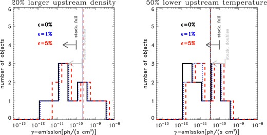
Left-hand panel: distribution of predicted γ-ray emission from our cluster sample, similar to Fig. 4 but here assuming a 20 per cent higher upstream gas density (left) compared to the basic model. Right-hand panel: as in the left-hand panel but assuming a 50 per cent lower upstream gas temperature compared to the basic model (see text for details). In both cases, we assume a capping of the magnetic field at 10 μG.
3.2.3 Radial dependence of the Mach number
Our assumption of a constant Mach number within the volume of interest follows from the assumption that the kinetic energy flux across shocks is conserved during their propagation. This implies that the dissipation of kinetic energy by these shocks is negligible, which is appropriate for the weak shocks considered here. Also the upstream medium is assumed to be isothermal (i.e. nu(r)(Mcs)3S(r)/2 = constant which gives M∝[nu(r) · S(r)]− 1/3 ≈ constant because nu(r) ∝ r−2 outside of the cluster core in the β-model). We also tested the possibility of a shallow radial dependence of the Mach number, M(r) = M0(r/Rrelic)1/2 (where M0 is the Mach number estimated at the location of the relic), as inVazza & Brüggen (2014). This was derived from the observed radial dependence of the radio spectral index of relics with radius (van Weeren et al. 2009). However, when only giant radio relics are considered, this trend is not significant (Bonafede et al. 2012; de Gasperin et al. 2014). To the best of our knowledge, the average radial trend of Mach number in clusters was discussed only by Vazza, Brunetti & Gheller (2009) and Vazza et al. (2010), and more recently by Hong et al. (2014). All these works confirm a very shallow functional dependence with radius of the average Mach number of shocks, typically going from M ∼ 1.5–2 in the centre to M ∼ 3 in the cluster periphery. This trend is consistent with M ∝ M0(r/rc)1/2 (with M0 ∼ 2). In Fig. 7, we show the results if we impose an M ∝ r1/2 instead of a constant Mach number. The predicted γ-ray emission downstream of relics is significantly reduced only in the single injection case (ϵ = 0), but the average emission of the sample still remains larger than both stacking limits. We conclude that the radial trend of Mach number with radius, as long as this is shallow as suggested by simulations, is not a crucial point. In the shock re-acceleration case, we also tested a scenario in which the re-acceleration is done by an M = 3 shock instead of the M = 2 as in our baseline model (Fig. 7, right). In this case, the requirement on the magnetic field are lowered and the number of relics for which we require Brelic ≥ 10μG is limited to one object (not shown). However, the predicted level of hadronic emission is now much increased and also the ϵ = 1 per cent run hits the Fermi stacking limits for this sample of objects, while the ϵ = 5 per cent now predicts an average emission which is ∼4–5 times larger than this.
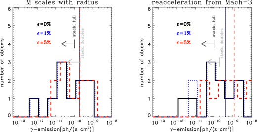
Left: distribution of predicted γ-ray emission from our cluster sample, similar to Fig. 4 but here considering a radial scaling of the Mach number downstream of relics, M(r) = M0(r/Rrelic)1/2. Right: same as in Fig. 4, but here assuming that the re-acceleration in the ϵ = 1 and 5 per cent cases is done by an M = 3 shock.
3.2.4 Mach number from the radio spectrum
The estimate of the Mach number at the position of relics is crucial in our modelling, as it determines the level of CR acceleration in the DSA scenario we are testing. However, several effects can make the Mach number we derive from the radio spectrum in Section 2.1 uncertain. In several observations, the Mach number derived from the radio spectrum is found to be higher than the one estimated through X-ray analysis (Akamatsu & Kawahara 2013; Ogrean et al. 2013). The surface of complex shocks is described by a range of values of Mach numbers rather than by a single value (Skillman et al. 2013) and the radio emission will be dominated by electrons probing larger Mach numbers compared to the mean (Hong et al. 2014). Additionally, radio observations with only a few beams across the relic can only produce integrated radio spectra, which are expected to be by ≈0.5 steeper than the injection spectrum. A blend of several populations of electrons seen in projection can yield spectra with time-dependent biases, as recently discussed by Kang (2015). To assess this effect, we run a set of Monte Carlo methods and extract uniform random deviates within M ± ΔM, where ΔM ≤ 0.5M. For each relic, we randomly extracted 200 values of ΔM and compute the downstream γ-ray emission in all cases. Fig. 8 shows the results for the single injection and re-acceleration models (coloured histograms). In this case, the simulated mean emission in the plot is the average of each set of 200 realizations (i.e. we first compute the mean emission for the cluster sample, for one random combination of extractions for ΔM, and then compute the average emission and dispersion within the full data set of 200 random realization). The number of 200 realization was chosen based on the fact that the errors in the mean emission do not change significantly for larger numbers of realizations. Compared to our fiducial model, a random variation in the assumed Mach number overall increases the level of hadronic γ-ray emission, suggesting that on average our baseline model underestimates the total emission. The underestimate is obviously more significant in the single-shock model (ϵ = 0), where the mean emission is ∼5 smaller than what we obtain as an average from the 200 random extractions. In the recceleration cases, the effect is smaller, and the fiducial model probably underestimates the hadronic emission by a factor of ∼1.5–2. For the same set of random extractions, the problem with requiring too large magnetic fields for a significant fraction of objects (∼1/3 in the ϵ = 0 and 1 per cent) remains (not shown). We conclude that realistic uncertainties in the Mach number do not change the robustness of our results.
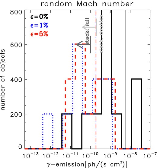
Distribution of predicted γ-ray emission from our cluster sample including a random deviate from the Mach number derived from the radio, in the range M = Mradio ± 0.5Mradio (see Section 3.2.4 for details). We extracted 200 random deviates for each object and computed the downstream hadronic emission for the three re-acceleration models. Differently from the previous figures, in this case the vertical lines show the mean emission from the 200 stacked samples (i.e. we computed the mean emission within the sample, one time for each random extraction, and then computed the mean emission over the 200 realizations).
3.2.5 Viewing angle
So far we assumed that all relics trace shocks which propagate exactly in a plane perpendicular to the line of sight. Numerical simulations of relics support this scenario and limit the inclination along the line of sight of the propagation plane down to ≤10–20 deg (van Weeren et al. 2011a; Kang et al. 2012). In general, simulated radio relics assuming DSA resemble the observational properties of most relics only when they lie close to the plane of the sky (Vazza et al. 2012b; Skillman et al. 2013). However, very small inclinations can be present and we checked if the inclusion of small (|Δω| ≤ 30 deg) along the line of sight can alter the picture in any significant way. Similar to the previous test, we randomly extracted 200 values of Δω for a uniform distribution in the ‘Bcap’ model, and accordingly recalculated the total volume spanned by shocks (which can only become bigger compared to the Δω = 0 case), and computed the average value of the 200 realizations of cluster stackings. Fig. 9 shows the results of this test. The average γ-ray emission from all realizations is of the order of the fiducial model (Δω = 0) and at the level of the Fermi stacking for this sample, and larger than the stacking by Ackermann et al. (2014). The outcome in the distribution of magnetic fields at relics is even worse than in the fiducial case, because in the case of large angles along the line of sight the relics are located further out, where the gas density is lower than in the Δω = 0 case, and the magnetic field must increase dramatically to match the radio power. As for all previous tests, we conclude that the presence of small but unavoidable projection effects has a small effect. However, on average these projection effects should yield an even larger hadronic emission from our data set if DSA is at work.
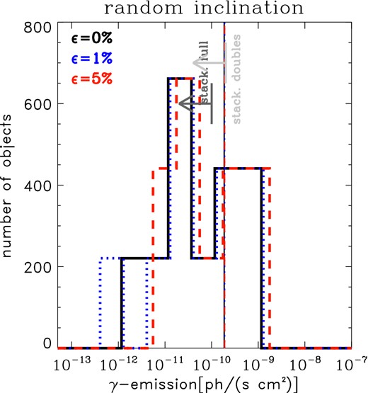
Similar to Fig. 8, but here by extracting 200 random values for the angle in the plane of the sky for each relic, |δω| ≤ 30 deg.
3.2.6 Uncertainties in CR physics
The efficiencies that we have tested produce the lowest amount of CR-acceleration (Kang & Ryu 2013). However, previously suggested functions for the η(M) acceleration efficiency (e.g. Kang & Jones 2007) give a larger injection of CRs from M ≤ 5 shocks, and can only make the problem with Fermi limits worse. Other uncertainties in the physics of CRs after their injection are briefly discussed here. Outside of cluster cores, the CRs are only weakly subject to hadronic and Coulomb losses, owing to the low gas density. For the sake of our analysis, it does not make any difference if they diffuse in the cluster volume at constant radius (since their contribution to the γ-ray emission only depends on the gas density and not on the exact location in the cluster atmosphere). Only diffusion in the vertical sense can change our estimate. However, this cannot be a big effect since CRs are thought to be frozen into tangled magnetic fields, and in this case their spatial diffusion is slow (i.e. τ ∼ 2 × 10⁸yr (R/Mpc)2 (E/GeV)− 1/3 for a constant B = 1 μG magnetic field and assuming Bohm diffusion, e.g. Berezinsky, Blasi & Ptuskin 1997). More recently, it has been suggested that the fast (vstreaming ≥ vA, where vA is the Alfvén velocity) streaming of CRs can progressively deplete the downstream region of the shock and reduce radio and hadronic emission (e.g. Enßlin et al. 2011), offering a way to reconcile hadronic models for radio haloes with the observed bimodality in the distribution of diffuse radio emission in clusters (Brunetti et al. 2007). However, the validity of this scenario is controversial (e.g. Donnert 2013; Wiener, Oh & Guo 2013) and this mechanism has been suggested to be maximally efficient in relaxed clusters. Instead, our sample of clusters with double relics is all made by objects with a very unrelaxed X-ray morphology. In the case of turbulent ICM, the detailed calculation by Wiener et al. (2013) shows that even fast streaming can also rapidly diminishes the γ-ray luminosities in the E = 300–1000 GeV energies probed by imaging air Cerenkov telescopes (MAGIC, HESS, VERITAS), but not in the lower energies probed by Fermi. Therefore, the latter is a more robust probe of the CR injection history, and our modelling here is well justified. Finally, our work neglects the (re)acceleration of CRs by other mechanisms, such as turbulent re-acceleration in the downstream of relics (e.g. Brunetti et al. 2004), which should re-energize radio emitting electrons as well as CR protons. Including this effect in our simple modelling is beyond the goal of this work; however, its net effect can only be that of further increasing the mean emission we predict here.
3.3 Other observational proxies: IC emission
Fig. 10 gives our predicted emission for the single injection case (blue) and for the extreme re-acceleration case (ϵ = 0.05), to emphasize the weak dependence of the predicted IC emission on the assumed re-acceleration model. Table 3 gives the predicted flux in IC emission from the downstream of all double relics in the [20-100] keV range, and the assumed radiative lengths in the downstream region. In all cases, the predicted emission lies below the detection threshold by the hard-X-ray satellite NUSTAR,6 which has been estimated to be of the order of a few ∼ 10− 12erg/(s cm2) in the case of the recent observations of the Coma cluster (Gastaldello et al. 2014) and of the Bullet cluster (Wik et al. 2014). However, a significantly lower sensitivity might be reached in the case of peripheral relics, given that in the latter clusters the contamination from the hot thermal gas in the hard-X-ray range hampers the detection of the IC signal. This might be the case for the most powerful targets in our sample, represent by A3376 (both relics) and by the most powerful relic in ZwCLJ2341. In these cases, the large distance from the centre of host clusters (∼1.2–1.3 Mpc) might indeed offer a better chance of detection of the IC signal. In the next years, the Astro-H satellite should be able to probe the IC emission in the same clusters (Awaki et al. 2014; Bartels, Zandanel & Ando 2015).
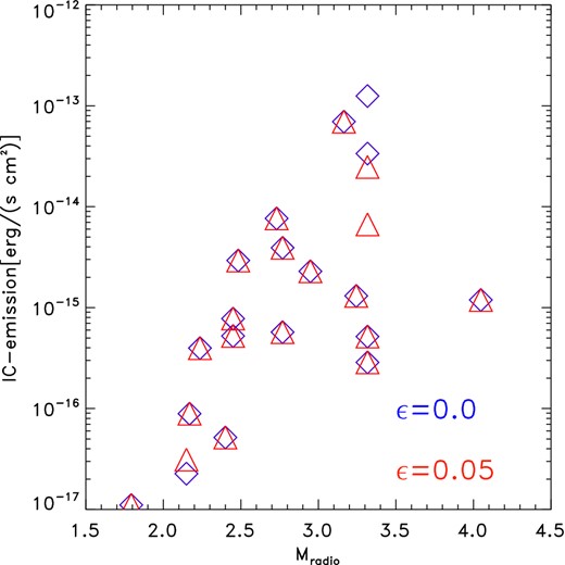
Forecast of IC emission from our simulated relics, in the extreme cases of ϵ = 0 (blue) and 0.05 (red).
Forecast of IC emission from the downstream region of relics in our simulated clusters, for [20–100] keV. The predictions are here only given for the ϵ = 0 using our model with a capping of the magnetic field at 10 μG, see Section 3.2.1 for details), as all others yield extremely similar results.
| Object | M1 | M2 | log10(eIC, 1) | log10(eIC, 2) | lcool, 1 | lcool, 2 | B1 | B2 |
|---|---|---|---|---|---|---|---|---|
| [erg/(s cm2)] | [erg/(s cm2)] | (kpc) | (kpc) | (μG) | (μG) | |||
| A3376 | 3.3 | 3.3 | −13.98 | −13.19 | 273.6 | 191.3 | 2.25 | 0.54 |
| A3365 | 2.1 | 1.8 | −16.78 | −18.78 | 87.6 | 48.6 | 5.41 | 8.69 |
| A1240 | 3.3 | 2.8 | −15.29 | −15.24 | 100.7 | 96.5 | 0.99 | 0.89 |
| A2345 | 2.8 | 2.2 | −14.41 | −15.40 | 107.2 | 131.1 | 0.60 | 0.97 |
| RXCJ1314 | 2.4 | 2.4 | −15.11 | −15.28 | 86.4 | 111.2 | 0.38 | 0.65 |
| MACSJ1149 | 3.3 | 2.4 | −15.54 | −16.29 | 101.7 | 96.4 | 1.75 | 1.46 |
| MACSJ1752 | 3.2 | 4.0 | −14.88 | −14.92 | 122.2 | 89.1 | 3.21 | 5.92 |
| A3667 | 1.7 | 3.8 | −14.53 | −14.12 | 164.4 | 159.7 | 1.56 | 1.32 |
| ZwCLJ2341 | 1.8 | 3.2 | −16.96 | −13.16 | 185.7 | 97.7 | 2.15 | 0.36 |
| PLCKG287 | 2.9 | 2.2 | −14.64 | −16.05 | 125.4 | 128.4 | 1.40 | 3.89 |
4 DISCUSSION AND CONCLUSIONS
Most of the evidence from X-ray and radio observations suggests a link between radio relics and merger shocks: merger axes of clusters and relic orientations correlate (van Weeren et al. 2011b), the power of radio relics scales with X-ray luminosities (Bonafede et al. 2012; Feretti et al. 2012) and mass (de Gasperin et al. 2014) of the host cluster. Cosmological simulations produce emission patterns consistent with observed radio relics just using a tiny fraction of the kinetic energy flux across shock waves (e.g. Hoeft et al. 2008; Pfrommer 2008; Battaglia et al. 2009; Skillman et al. 2011, 2013; Nuza et al. 2012; Vazza et al. 2012b).
Still, a number of recent observations have revealed some open issues, including uncertain merger scenarios (e.g. Ogrean et al. 2013), departures from power-law spectra (e.g. Stroe et al. 2014; Trasatti et al. 2015), missing associations between radio emission and X-ray maps (e.g. Russell et al. 2011; Ogrean et al. 2014), efficiencies problems (e.g. Macario et al. 2011; Bonafede et al. 2012), inconsistencies between Mach numbers derived from X-ray and radio observations (e.g. Kale et al. 2012; Akamatsu & Kawahara 2013; Ogrean & Brüggen 2013) and apparent connections to radio galaxies (Bonafede et al. 2014).
In this work, we used a simple semi-analytical model of expanding merger shocks in clusters to reconstruct the propagation history of shocks leading. We used a spherically symmetric model and assumed that CR protons are trapped in the ICM on all relevant time-scales. A range of realistic scenarios for the acceleration of relativistic electrons and protons via DSA, varying the upstream gas conditions, the shock parameters and the budget of pre-existing CRs, gives very similar results. In all realistic scenarios, a significant fraction of our objects (∼1/2–1/3) has difficulties in matching at the same time the observed radio emission and the constraints imposed by the Fermi limits, unless the magnetic field in all problematic objects is much larger than what usually considered realistic ( ≫ 10 μG). The scenario in which radio emitting electrons comes from the re-acceleration of pre-existing electrons (Kang et al. 2012; Pinzke et al. 2013) can alleviate the tension with Fermi if the pre-existing electrons are not the result of previous injection by shocks as we investigated here, but are instead released by mechanisms that mostly inject leptons (e.g. leptonic-dominated jets from AGN), as already discussed in Vazza & Brüggen (2014).
Based on our semi-analytical model, the standard DSA scenario with thermal leakage that predicts that ECRe ≪ ECRp cannot simultaneously explain radio relics and produce less γ-radiation than the upper limits from Fermi, unless unrealistically large magnetic fields are assumed at the position of relics (e.g. Brelic ≥ 10-100 μG). This result is very robust, at least in the statistical sense, against all investigated variations of our fiducial parameters for the modelling of the shock acceleration of CRs. Additional effects that go beyond our idealized modelling of cluster mergers, e.g. a clumpy ICM, a succession of mergers and the additional acceleration of CRs by AGN, supernovae, turbulence or reconnection exacerbate this discrepancy.
Despite its obvious degree of simplification, a semi-analytical method is useful to tackle the case of double-relic systems. In these systems, it is reasonable to assume that most of the energetics is related to the observed pair of giant merger shocks. Their shape and location is rather regular and symmetric with respect to the cluster centre, suggesting that one can make reasonable estimates for their propagation history. This setup allows us to run very fast testing of different possible acceleration scenarios, and as we showed in our various tests it generally gives a lower limit on the expected γ-ray emission. This method is meant to be complementary to fully cosmological numerical simulations where the effects of multiple shocks, particle advection and cooling, as well as inputs from galaxy formation and other mechanisms can be taken into account at run-time (e.g. Pfrommer et al. 2007; Vazza et al. 2012a). However, a thorough exploration of models is computationally demanding because of the required high resolution and the complexity of the numerics. Also the agreement between different numerical techniques on this topic is still unsatisfactory (see discussion in Vazza et al. 2011b).
Another way of illustrating our result is found by rescaling the efficiency for proton acceleration, η(M), such that the upper limits from Fermi are not violated. In the case without pre-existing CRs, this is a simple exercise as we only need to rescale η(M) for each relic separately, and compute the average of the efficiencies for each bin of the Mach number (here we chose a bin size of ΔM = 0.6 to achieve a reasonable sampling of the sparse distribution of Mach numbers in the data set). Here, we keep the magnetic field fixed at B = 2 μG as suggested by recent observations (de Gasperin et al. 2014). The result is shown in Fig. 11, where we show the maximally allowed acceleration efficiency for CR-electrons, protons, as well as Ke/p as a function of M. This relation results from a somewhat coarse simplification of the problem but it is a rough estimate of the acceleration efficiencies in weak ICM shocks.
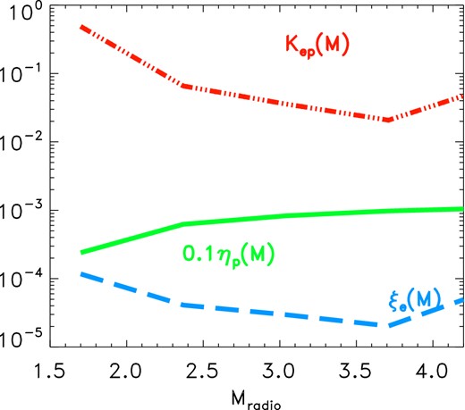
Acceleration efficiency of CR-protons (green, rescaled by a factor × 10 down) and CR-electrons (blue), and electron to proton acceleration ratio (red) allowed by our combined radio and γ-ray comparison with observations. In this case, we assumed a fixed magnetic field of B = 2μG for all relics.
For shocks with M ≤ 2, the flux ratio of injected electrons is larger than that in protons, Ke/p ∼ 1–100, at odds with standard DSA (even including re-accelerated electrons). For M ≥ 2.5 the acceleration efficiency of protons can become significant (∼10−3–10−2), while the acceleration efficiency of electrons flattens and Ke/p ∼ 10−2. The functional shape of the acceleration efficiency for protons is consistent with the (Kang & Ryu 2013) model, but the absolute normalization is lower by a factor of ∼10–100. A value of Ke/p larger than what usually assumed by DSA was already implied by our first work (Vazza & Brüggen 2014), and has been later suggested by other authors (Brunetti & Jones 2014).
A possible solution has been suggested by Kang et al. (2014), who assumed that electrons and protons follow a κ-distribution near the shock transition. A κ-distribution is characterized by a power law rather than by an exponential cutoff at high energies, thus ensuring a more efficient injection of high-energy particles into the DSA cycle. This distribution is motivated by spacecraft measurements of the solar wind as well as by observations of H ii and planetary nebulae (e.g. Lazar et al. 2012, and references therein). Kang et al. (2014) explored the application of the κ-distribution to M ≤ 2 shocks in the ICM, and concluded that the distribution can have a different high-energy tail as a function of the shock obliquity and of the plasma parameters. In the ICM, the distribution might be more extended towards high energies for electrons than for protons thus justifying a higher acceleration efficiency for electrons than for protons. However, in order to explain the origin of these wider distributions, one must resort to detailed microphysical simulations of collisionless shocks.
The most promising explanation for the non-observation of γ-rays has been suggested by Guo, Sironi & Narayan (2014), who studied the acceleration of electrons with PIC simulations under conditions relevant to merger shocks. They showed that M ≤ 3 shocks can be efficient accelerators of electrons in a Fermi-like process, where electrons gain energy via shock drift acceleration. The electrons gain energy from the motion of electric field and scatter off oblique magnetic waves that are self-generated via the firehose instability. They found that this mechanism can work for high plasma betas and for nearly all magnetic field obliquities. However, these simulations have been performed in 2D, and could not follow the acceleration of electrons beyond a supra-thermal energy because of computing limitations. At the same time, hybrid simulations of proton acceleration by Caprioli & Spitkovsky (2014) have shown that the acceleration efficiency is a strong function of the obliquity angle. If indeed the magnetic field in radio relics is predominantly perpendicular to the shock normal, as found e.g. in the relic in the cluster CIZA 2242.2+5301, then the prediction is that the acceleration efficiency of protons is strongly suppressed, thus explaining the non-detection of hadronic emission. It remains to be seen if the results of these simulations hold in 3D, with realistic mass ratios between electrons and protons and coupled to a large scale MHD flow. It is also not clear whether the magnetic field is quasi-perpendicular in all the relics of this sample and how the alignment of the magnetic fields with the shock surface observed on large scales can be scaled down to scales of the ion gyro radius.
FV and MB acknowledge support from the grant FOR1254 from the Deutsche Forschungsgemeinschaft. DE and BH thank Andrea Tramacere and Christian Farnier for their help with the development of the Fermi tools. We acknowledge fruitful scientific discussions with F. Zandanel, A. Bonafede, F. Gastaldello, T. Jones and D. Wittor for this work.
Instead, since the Larmor radius of thermal electrons is much smaller than the typical shock thickness, thermal electrons cannot be easily accelerated to relativistic energies by DSA. This so-called injection problem for electrons is still largely unresolved (e.g. Brunetti & Jones 2014).
We notice that, compared to the original equation by Hoeft & Brüggen (2007), we use here upstream values for density and temperature, as the function η(M) also accounts for the shock compression factors. As in Hoeft & Brüggen (2007), the fields in the equation are normalized as follows: ne/[10− 4 cm3], T/[7 keV], B/[μG], S/[Mpc2] and ∋/[1.4 GHz].
http://fermi.gsfc.nasa.gov/ssc/data/analysis/software/aux/gal_2yearp7v6_v0.fits. As in Hoeft & Brüggen (2007), the fields in the equation are normalized as follows: ne/[10− 4 cm3], T/[7 keV], B/[μG], S/[Mpc2] and ∋/[1.4 GHz].
In this case, the values of ϵ = 0, 1 and 5 per cent quoted in the labels actually refer to the initial assumed value for each cluster, while the final value depends on the iterations described here. However, in all cases the iterations stopped after reaching ϵ ∼ a few per cent.
