


Abstract
In this work, we study two specific characteristics of the Phocaea region. First, we analyse the presence of the secular resonances involving the inner planets. Our results show that some of these are present, and relevant for the dynamics of asteroids in this region. The most important seems to be the s − s4 + g3 − g7 resonance. Secondly, we study the role of the 7/2 mean motion resonance with Jupiter as a border of the region in terms of semimajor axis. In particular, we check whether or not this resonance could be crossed under the combined influence of gravitational and non-gravitational forces. The obtained results show that a significant fraction of our test particles successfully transit across the resonance, without being removed from the region. Moreover, we found that most of the asteroids below a few hundred metres in diameter should be able to cross the 7/2 resonance. This means, despite being relatively effective in pumping up asteroid eccentricities in this region, this resonance is not an absolute dynamical boundary.
1 INTRODUCTION
The Phocaea group, named after its first discovered member, namely asteroid (25) Phocaea, is located in the inner part of the main asteroid belt. It consists of objects having orbital semimajor axis stretching from about 2.25 to 2.5 au, inclination higher than about 20 deg and eccentricity ranging between 0.15 and 0.3. This region is characterized by a very interesting dynamics; thus, it has been subject of different studies in the past (e.g. Knežević & Milani 2003; Carruba 2009, 2010; Michtchenko et al. 2010).
The Phocaea group is known to have dynamical boundaries surrounding it from all sides but one, thus separating it almost completely from the rest of the main belt. In terms of semimajor axis it is delimited by two mean motion resonances (MMRs) with Jupiter. An inner boundary is often linked to the 7/2 resonance located at about 2.25 au, and an outer border is set by the 3/1 MMR located at 2.5 au. Moreover, the region is delimited by important secular resonances (SRs): the ν6 = g − g6 at low inclination, and the ν5 = g − g5 and ν16 = s − s6 at high inclination1 (Knežević et al. 1991; Michtchenko et al. 2010). Besides, although deep close encounters with Mars are not possible due to the Kozai class protection mechanism (Milani et al. 1989), as discussed in Knežević & Milani (2003) shallow encounters could occur, and these may result in removal of asteroids for eccentricities higher than about 0.3. These are the most important dynamical mechanisms which separate the Phocaea group from the rest of the main belt. The only side at which dynamical boundary does not exist is towards lower eccentricities.
The value of the semimajor axis where sharp drop in number density occurs coincides with the location of the 7/2 resonance. Thus, as mentioned above, this resonance is often assumed to be dynamical boundary preventing asteroids from the Phocaea region to drift closer to the Sun. However, to our knowledge, this assumption has never been studied in great details.
Morbidelli & Nesvorny (1999) analysed diffusion tracks in the inner main belt and found the 7/2 to be efficient in pumping up orbital eccentricities, what leads to close approach with Mars, thus, making this resonance as one of the main sources of Mars crossers. Still, these authors noted that there is another resonance almost at the same location as 7/2: that is 5/9 MMR with Mars. Furthermore, Morbidelli & Nesvorny (1999) even found that 5/9 with Mars is more important than 7/2 with Jupiter.
More recently, the 7/2 resonance was studied by Carruba (2010) who analysed the dynamical erosion of asteroid groups in the region of the Phocaea family. This author also found that the 7/2 could significantly increase the eccentricities of captured objects.
Despite these findings it is important to underline that Morbidelli & Nesvorny (1999) did not consider the role of the Yarkovsky effect, which could reduce the time spent inside the resonance, thus, making chaotic diffusion less efficient. This could be particularly relevant for smaller asteroids which are subjects of fast, Yarkovsky-induced, drift in semimajor axis. On the other hand, Carruba (2010) did take into account Yarkovsky effect in his simulations, but the results are obtained on a statistically small sample.
For the above-mentioned reasons, we believe that additional investigation is necessary to examine precisely the role of the 7/2 resonance with Jupiter, both, as a border of the Phocaea region and as a source of Mars crossers. Thus, in this paper, we extend the previous studies related to the 7/2 MMR with Jupiter, aiming mainly to study the role of this resonance in stopping asteroids from the Phocaea region on their route towards the Sun. This analysis is performed considering combined effect of gravitational and non-gravitational perturbations. As we show in this paper, the 7/2 resonance is not an absolute dynamical boundary for sufficiently small objects, below some hundred metres in diameter.
Moreover, we have also analysed the role of SRs involving the inner planets, for the dynamics of asteroids belonging to this region.
2 PHOCAEA GROUP
2.1 Some basic facts
Phocaea group has currently about 4000 known asteroids. As the first step in our analysis, we compute proper orbital elements for 3164 numbered and 938 multi-opposition asteroids from, and close to, the region, using the method developed by Knežević & Milani (2003). Their distributions in the (ap,ep) and (ap,sin (Ip)) planes are shown in Fig. 1.
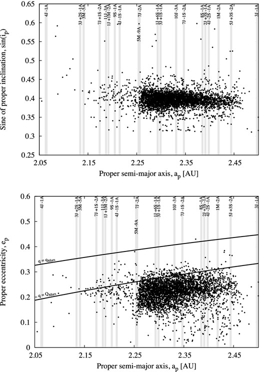
Distributions of 4102 asteroids located near and inside the Phocaea region, shown in the (ap,sin (Ip)) and (ap,ep) planes. The vertical strips represent approximately the locations of the most important two- and three-body MMRs. The relations q = QMars and q = qMars, where q and Q are the perihelion and aphelion distances, respectively, are also shown in the (ap,ep) plane.
From dynamical point of view, let us recall that many MMRs as well as some SRs cross this region. The locations of a number of MMRs are shown in Fig. 1. Despite the fact that there are many of them, most MMRs are weak and play only a minor role in the dynamics of the Phocaea group. Still, some of them (e.g. the 1/2 with Mars) cause evolution of proper eccentricity, and contribute to sustain a high-eccentricity population in this region (Carruba 2010). Simulations performed by this author show that this resonance can either increase or decrease orbital eccentricity, but in most cases the effect is an actual pumping up of eccentricity. In particular, it was found that for some asteroids the eccentricity can increase by as much as 0.15 in 200 Myr. However, no trace of a vertical alignment of asteroids currently experiencing an increase of eccentricity due to the 1/2 MMR with Mars can be seen in Fig. 1. The reason could be a quick removal of these bodies due to moderately close encounters with Mars.
Most of the Phocaea asteroids have spectra similar to that of S-type asteroids (Carvano et al. 2001), typical for objects located in the inner main belt. The available data provided by the Sloan Digital Sky Survey (Ivezić et al. 2001) suggest that more than 70 per cent of Phocaea asteroids belong to the S-type (Novaković, Cellino & Knežević 2011), yielding the same conclusion. Similarly, the albedos obtained within the Wide-field Infrared Survey Explorer project (Masiero et al. 2011) range from 0.15 to 0.4 for about 70 per cent of the observed objects, in agreement with the inferred S spectral type. Still, the latter survey found about 20 per cent objects with albedo below 0.1.
A possible existence of collisional families inside the Phocaea region has been discussed by several authors (e.g. Gil-Hutton 2006; Carruba 2009; Novaković et al. 2011). These authors found several candidate groups that pass statistical significance criteria, thus, which may be real collisional families. However, due to the peculiar characteristics of this region, the situation is not very clear. The candidate Phocaea family includes most asteroids present in the region. Therefore, it is difficult to discriminate whether we deal here with a really collisional outcome or rather with a group of asteroids trapped inside an island of stability. The difficulties encountered in interpreting the Phocaea region generally bear resemblance with those already met in analysing the Hungaria region (Milani et al. 2010), but the situation here seems to be even more difficult. Thus, despite some evidence supporting hypothesis that the Phocaea family is real, its existence is still to be confirmed. Moreover, the membership of this supposed family is also uncertain, as well as its most likely age estimated to be up to 2.2 Gyr (Carruba 2009).
2.2 Secular Resonances in the Phocaea region
One of the main purposes here is to investigate a possible role of SRs involving the inner planets, for the dynamics of asteroids from the Phocaea region.
The locations of SRs projected on the semimajor axis versus eccentricity (inclination) plane depend on the assumed value of inclination (eccentricity). This may be particularly important at high orbital inclinations (Knežević et al. 1991). Thus, for sets of objects having a significant difference between highest and lowest eccentricity (or inclination) value, the locations of SRs at these extremes may be quite different. Therefore, it is easier to plot locations of SRs in the (g, s) plane, and we adopt this approach here.
The distribution of asteroids from the Phocaea region in the plane of proper frequency g of the longitude of perihelion versus proper frequency s of the longitude of node is shown in Fig. 2. Using this figure it is easy to confirm several known facts. The dynamical borders of the Phocaea region caused by major SRs are clearly visible in the plot. Also, the interaction of asteroids belonging to this region with the g − g6 − s + s6, g − g5 + s − s6 and g − g6 − 2s + 2s6 SRs can be recognized by the alignments of objects associated with these resonances.2
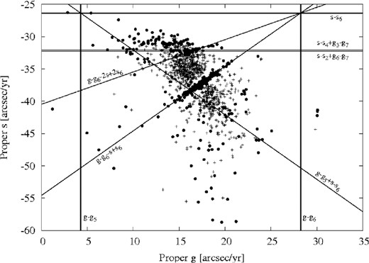
The asteroids in the Phocaea region plotted in the plane of proper frequency g of the longitude of perihelion versus proper frequency s of the longitude of node. The objects with σe and σsinI less than 0.002 are plotted as crosses, while objects with larger errors are plotted as full circles. The lines show the locations of several SRs which are indicated in the plot. The alignments of objects that are apparent in the figure are artefacts produced by averaging over periods longer than a libration period of the corresponding SR.
As we already mentioned, our main purpose here is to check a possible role of SRs with the inner planets. However, the values of secular frequencies of the inner planets (see Laskar 1990) are such that numerous resonant combinations exist very close to each other. This makes a study of the role of a single resonance very complex. Accordingly, instead of aiming to identify and analyse all SRs with the inner planets present in the region, we focused here on a few interesting examples. In selecting these examples we were mainly motivated by the features visible in Fig. 2, i.e. by the alignments of objects around s = −32 arcsec yr−1, which could not be explained in terms of SRs involving the outer planets only. Moreover, we limited our analysis to the resonances that are up to order 4 (i.e. they arise from the perturbing terms of degree of at least 4 in eccentricity and inclination; Knežević et al. 1991; Milani & Knežević 1990).
In Table 1, we listed several SRs with the inner planets. Following Carruba et al. (2014), we provide here, along with the resonant combinations and exact values of resonant frequencies, a number of likely resonant objects, i.e. the asteroids within ±0.1 arcsec yr−1 from the resonance centre in space of proper frequencies. The limit of 0.1 arcsec yr−1 is adopted based on the fact that for a stronger SR, namely the z1 = g − g6 + s − s6, usually the criterion of ±0.3 arcsec yr−1 is used (Carruba et al. 2014). Certainly, the fact that an asteroid is a likely resonator does not necessarily imply that it is locked inside a resonance. Still, this is a good way to find potential candidates, and to get a preliminary assessment of the relevance of this resonance.
Examples of secular resonances, involving inner planets, present in the Phocaea region. In columns are given resonant combinations, frequency values and number of likely resonant asteroids.
| Resonant combination | Frequency (arcsec yr−1) | Number of resonators |
|---|---|---|
| s − s3 + g3 − g5 | s = −31.89 | 20 |
| s − s4 + g3 − g7 | s = −31.97 | 21 |
| s − s2 + g6 − g7 | s = −32.21 | 24 |
| s − s3 + g4 − g5 | s = −32.44 | 25 |
| s − 2s4 + s7 | s = −32.53 | 27 |
| s − s4 + g4 − g5 | s = −31.35 | 18 |
| g − g2 − s4 + s6 | g = 16.04 | 47 |
| g − g5 − s2 + s3 | g = 16.06 | 42 |
| g − g5 − s2 + s4 | g = 14.97 | 39 |
| g − g3 + g7 − g8 | g = 14.89 | 52 |
| g − g8 + s − s4 | g + s = −17.09 | 32 |
To better understand which resonances are responsible for the alignment of objects around s = −32 arcsec yr−1, we have analysed the behaviour of the resonant critical angles of the three closest SRs, namely s − s3 + g3 − g5, s − s2 + g6 − g7 and s − s4 + g3 − g7. We have found evidence that each of these three resonances affects some of the asteroids in the Phocaea region. However, these interactions do not seem to be stable, i.e. they do not last for a long time.
As an example, in Fig. 3 we show the evolution of the resonant critical angle of the s − s4 + g3 − g7 resonance for asteroid (2696) Magion. Although long intervals of circulation with different speeds can be seen, the resonant angle spends a non-negligible amount of time in libration state. Thus, although some caution is needed, this result suggests that SRs involving the inner planets may be important for the dynamics over long time-scales of the asteroids in the Phocaea region.
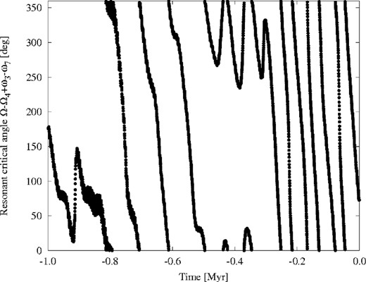
Time evolution of the resonant critical angle of the s − s4 + g3 − g7 SR for asteroid (2696) Magion. The critical angle is obviously in a libration state starting from about −0.3 to −0.5 Myr.
As a next step of our analysis, we investigated how the same critical angles behave when the Yarkovsky thermal force is considered. Thus, we integrate several representative asteroids again, but this time including the Yarkovsky effect in the dynamical model. These integrations were repeated three times assuming three different values of Yarkovsky-induced drift in semimajor axis, namely 1 × 10⁻⁴, 1 × 10⁻³ and 1 × 10⁻² au Myr−1.
Interestingly, the behaviours of the critical angles were practically the same with or without Yarkovsky effect included in the model (see Fig. 4). This means that the thermal force is not very efficient in removing objects from the s − s4 + g3 − g7 resonance. An explanation might be that the evolution of the secular angles is controlled by an eccentricity cycle, rather than the evolution of semimajor axis. Certainly, this conclusion is based on a relatively short integration time span of 1 Myr, and should be treated with caution. Still, the fact that the outcome remains the same, even for the unrealistically high value of Yarkovsky drift of 1 × 10⁻² au Myr−1, suggests that the s − s4 + g3 − g7 SR indeed may have some role in the long-term dynamical evolution of asteroids in the Phocaea region.
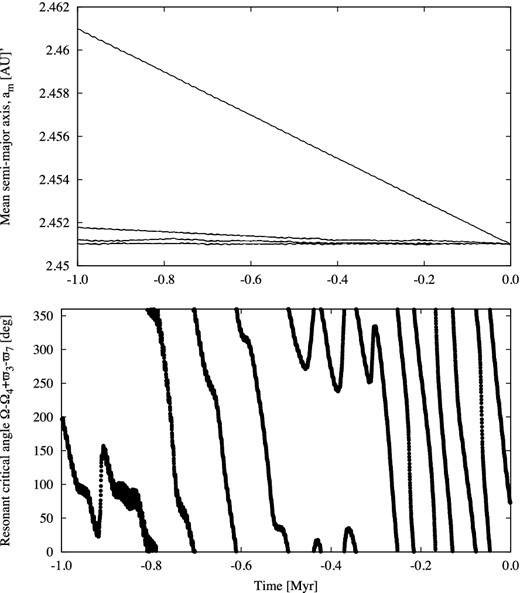
The effect of the Yarkovsky thermal force in the semimajor axis and the resonant critical angle of the s − s4 + g3 − g7 resonance, for asteroid (2696) Magion. In the upper panel, the time evolution of the mean semimajor axis without Yarkovsky and for three different values of Yarkovsky drift is shown. The bottom panel shows the behaviour of critical angle when the fastest Yarkovsky drift of 1 × 10⁻² au Myr−1 is assumed. See the text for additional explanations.
3 THE INNER BOUNDARY OF THE PHOCAEA REGION
Our main purpose here is to study in more detail the dynamical behaviour of objects close to or inside the 7/2 resonance and to explore the dynamical consequences for objects possibly subject to a Yarkovsky-driven drift in orbital semimajor axis, to be led to cross this resonance. For this purpose we adopted two approaches, both based on a set of numerical integrations of test particles.
3.1 Methodology
In all cases, the orbital motion of our test bodies was tracked for 20 Myr using the public domain orbit9 software (Milani & Nobili 1988) embedded in the multipurpose orbfit package.3 The dynamical model includes seven planets, from Venus to Neptune, as perturbing bodies. To account for the indirect effect of Mercury, its mass is added to the mass of the Sun and the barycentric correction is applied to the initial conditions.
In most of the simulations, the Yarkovsky thermal force was also included in the model. The Yarkovsky force is a consequence of a radiative mechanism related to the absorption and re-emission of solar radiation. It primarily produces a drift in semimajor axis and it depends on several parameters, including size, thermal inertia and orientation of the spin axis. It varies as 1/D, where D is the body's diameter (Rubincam 1995; Farinella & Vokrouhlicky 1999; Bottke et al. 2001).
For sake of simplicity, we approximated the Yarkovsky effect in terms of a pure along-track acceleration, producing the same average semimajor axis drift da/dt as expected from the theory of the Yarkovsky effect (Vokrouhlicky 1998; Vokrouhlický 1999). In these simulations, we assumed different da/dt rates. In particular, we chose the following values: −1.0 × 10⁻⁴, −2.5 × 10⁻⁴, −5.0 × 10⁻⁴, −7.5 × 10⁻⁴, −10.0 × 10⁻⁴ and −15.0 × 10⁻⁴, all the above values being expressed in au Myr−1. These drift rates approximately correspond to a maximum drift expected for S-class asteroids having sizes of 2.9, 1.2, 0.6, 0.4, 0.3 and 0.2 km, respectively. This is valid at heliocentric distances corresponding to the Phocaea region, by assuming for all objects the following parameters: geometric albedo identical to that of (25) Phocaea, 0.231, according to Tedesco et al. (2002), low-surface thermal conductivity 0.001 W m−1 K−1, thermal capacity 680 J kg−1 K−1, thermal emissivity 0.95 and bulk density of 2.5 g cm−3 (e.g. Bottke et al. 2006).
Two approaches used here are in many ways similar, but there are some important differences. The main difference is that in the first method we work with osculating and mean elements, while for the second method we adopt to work with proper orbital elements. Thus, we decided to treat these as two different methods.
3.1.1 The first method
Our first method to study the 7/2 resonance consists of four main steps. First, we determine the outer border of the resonance in terms of semimajor axis, taking into account a fact that the width of an MMR is proportional to the eccentricity. Secondly, once the outer boundary is defined, we chose the initial conditions for 20 000 test particles in such a way to resemble the shape of the resonance in the semimajor axis versus eccentricity plane. Thirdly, these test particles are integrated using the dynamical model that includes the Yarkovsky effect, forcing them all to drift inwards, i.e. towards the 7/2 resonance. Finally, we define the criteria for the resonance crossing and analysed the output of the numerical integrations.
The outer border of the resonance for four different intervals of orbital eccentricities is determined using the trial-and-error approach. That is, we placed some objects near the expected location of the resonance border, and check whether they are inside the resonance or not. Based on the limits obtained in this way, we generate the initial conditions of our test particles. Assuming that within the one interval of eccentricity the border of the resonance in the a–e plane could be described as a line, we placed the initial positions of 1000 particles along these four lines. Thus, the osculating eccentricities are equally distributed in each of four intervals [0.0, 0.10], [0.10, 0.15], [0.15, 0.20], [0.20, 0.30]. Then, as the lines follow the outer (entering) boundary of the resonance, the osculating semimajor axes are chosen in intervals [2.258 05, 2.258 475], [2.258 475, 2.259 075], [2.259 075, 2.259 775], [2.259 775, 2.261 075], but in such a way to satisfy the relation e = ka + n in each segment of a and e.
The orbital inclinations are generated randomly within the interval [18°, 29°], which corresponds to the inclinations of the objects from the Phocaea region. Three remaining angles, the longitude of node, the longitude of perihelion and the mean anomaly, are all picked up randomly4 from the interval [0°, 360°].
To each of these 1000 particles generated in the previous step, we assign 20 different values of the Yarkovsky drift. In this case, the Yarkovsky drift varies from −5.0 × 10⁻⁵ to −1.0 × 10⁻³ au Myr−1 with the step of −5.0 × 10⁻⁵ au Myr−1. As a result, we produced an input catalogue with 20 000 fictitious objects in total.
The next step is to adopt criteria for the resonance crossing. For this purpose, we define two conditions that must be satisfied to consider that a particle crossed the 7/2 resonance. The first condition is based on a location of the inner (exiting) border of the resonance in the a–e plane, and it could be defined applying the same logic as in the definition of the position of the outer (entering) border, but this time using mean orbital elements and seven different intervals in eccentricity. The exact values used for this condition are listed in Table 2.
The criteria for the first condition of the 7/2 resonance crossing as a function of the mean semimajor axis am and mean eccentricity em.
| 1 | |$0.35 \le e_{m}, \hspace{37.0pt} a_{m} < 2.2520$| |
| 2 | |$0.30 \le e_{m} < 0.35, \hspace{7.0pt} a_{m} < 2.2525$| |
| 3 | |$0.25 \le e_{m} < 0.30, \hspace{7.0pt} a_{m} < 2.2530$| |
| 4 | |$0.20 \le e_{m} < 0.25, \hspace{7.0pt} a_{m} < 2.2535$| |
| 5 | |$0.15 \le e_{m} < 0.20, \hspace{7.0pt} a_{m} < 2.2540$| |
| 6 | |$0.10 \le e_{m} < 0.15, \hspace{7.0pt} a_{m} < 2.2545$| |
| 7 | |$0.00 \le e_{m} < 0.10, \hspace{7.0pt} a_{m} < 2.2550$| |
The second condition is based on a trend in the evolution of the semimajor axis and its comparison with a trend expected due to the Yarkovsky-induced drift. Thus, to define this criterion, we apply the linear least-squares method to fit time series of the mean semimajor axis. The fitting is performed using the time span of at least 0.75 Myr and at most 1 Myr, starting from the moment when the first condition is fulfilled. From the fit we calculate the parameters k, n of a linear model am = kt + n, and their corresponding errors σk, σn. Using the results from the fit, the second condition is then defined with three related sub-conditions. These are as follows.
The coefficient k of the best-fitting line must be negative; this is to be in agreement with the adopted Yarkovsky drift.
The ratio between coefficient k and its error σk has to be greater than 30; this is to ensure that we are using only reliable values of k.
Slope of an adopted Yarkovsky drift speed of a test particle must be in the interval (k − σk, k + σk); this is to confirm that evolution is a consequence mainly of the Yarkovsky drift, meaning that interaction with the resonance is not taking place.
Thus, if each of the three sub-conditions is satisfied, we consider the second criterion to be fulfilled. Finally, if a test particle meets both two conditions, we consider that this object crossed the 7/2 resonance.
All analyses related to our first method are performed on mean orbital elements, which are mostly free from the short periodic perturbations. The mean elements are obtained directly from the orbit9 integrator which has an option to perform online digital filtering in order to remove short periodic oscillations. The obtained results are presented in Section 3.2.
3.1.2 The second method
The second method is in many aspects similar to the first one, and it is also based on the numerical integrations of test particles. The main difference is that here we used proper orbital elements instead of the osculating or mean elements.
The initial positions of test particles are this time chosen in a slightly different way. They are again initially placed close to the outer boundary of the 7/2 resonance, but instead to follow exactly the border of the resonance, we decide here to resemble the orbit of a real asteroid. In particular, the osculating semimajor axes, eccentricities and inclinations were generated, with random values within the intervals 2.257–2.258 au in semimajor axis, 0.172–0.173 in eccentricity and 21| $_{.}^{\circ}$|8–21| $_{.}^{\circ}$|9 in inclination. Orbital elements generated in this way are similar to those of the asteroid (106767) 2000XW13, a real object very close to the 7/2 MMR.
Seven sets of the integrations are performed, using 100 test particles in all cases. The first set of integrations is performed by using a purely gravitational model. In the remaining six sets of simulations, a Yarkovsky thermal force is also included in the model, and different sets correspond to different assumed values of the Yarkovsky drift speed (see Section 3.1).
By means of our numerical integrations, we were able to extract two main results. First, for each of the sets we determined the fraction of bodies that were removed during the simulated 20 Myr time span. Here, we consider as ‘removed’ those objects which either are ejected from the Solar system or fall into the Sun.
Secondly, we determined the fraction of objects that were able to cross the 7/2 resonance during the same time span. More precisely, we worked here in terms of proper elements, in order to make sure that resonance crossing was not just temporary, i.e. due to temporary oscillations of the osculating (or even mean) elements.
In particular, using the last 10 Myr of integrations, we computed synthetic proper elements for all 100 fictitious objects and for each of seven different sets of integrations. Then, we determined the number of asteroids that eventually crossed the 7/2 resonance, but taking into account only those bodies having proper perihelion distance greater than aphelion distance of Mars at the end of the integrations, because objects having larger eccentricity can have close encounters with Mars and are expected to be removed from the Phocaea region. Here the criterion for the resonance crossing is based only on the value of proper semimajor axis. Still, in the case of proper elements this is a safe approach, because resonant objects typically show alignment in the a–e (or a–i) plane, thus, making distinction between resonant and non-resonant objects relatively easy.
3.2 Results
3.2.1 Results obtained using the first method
Here we present the results obtained by applying the first method of the above-described methodology.
Let us first show two examples of the test particles that successfully crossed the 7/2 resonance. In Fig. 5, an example of a test particle which very quickly crossed the resonance is shown. Actually, this particle crossed the resonance almost instantaneously, although the adopted Yarkovsky drift speed is not very fast, i.e. only −2.5 × 10⁻⁴ au Myr−1.
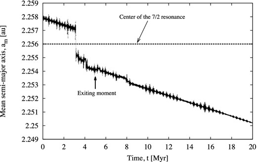
An example of test particle which quickly crossed the 7/2 resonance. Its adopted Yarkovsky drift speed is −2.5 × 10⁻⁴ au Myr−1, while the inferred fitting parameter k is ≈−2.46 × 10⁻⁴ au Myr−1, and its corresponding error σk ≈ 3.9 × 10⁻⁶ au Myr−1. The moment of crossing is at t ≈ 5.0 Myr, marked by an arrow.
The second example of the resonance crossing, shown in Fig. 6, is a bit different from the first one. This particle entered the resonance at about 2 Myr, and remains captured for about 15 Myr, before it finally exits from the resonance at about 17 Myr. This is a very interesting example, because despite its relatively fast Yarkovsky drift speed of −4.0 × 10⁻⁴ au Myr−1, it spends a long time inside the resonance.
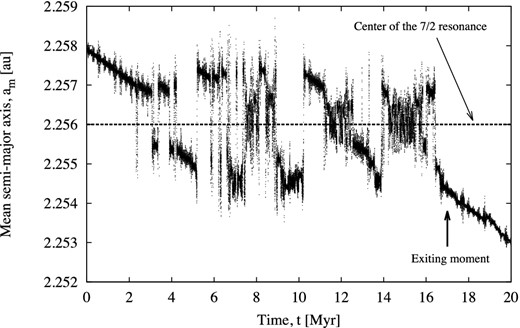
The same as in Fig. 5, but for a particle with Yarkovsky drift speed −4.0 × 10⁻⁴ au Myr−1, k ≈ −4.03 × 10⁻⁴ au Myr−1, σk ≈ 3.2 × 10⁻⁶ au Myr−1. The moment of crossing is at t ≈ 17.0 Myr, shown by an arrow.
These two examples demonstrate how our criteria for the resonance crossing work, but also show that for single objects the time spent in the resonance may not directly depend on the Yarkovsky drift speed.
However, for our study the statistical approach matters the most, rather than the results obtained for single test particles. Thus, in Figs 7 and 8 we show the distribution of the instants of the resonance crossing for all test particles. More precisely, in Fig. 7 we show this distribution for all test particles that successfully crossed the resonance, regardless whether or not they have close approach to planets. On the other hand, in Fig. 8 are shown only results for particles which did not have a close approach to planets.
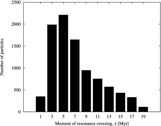
Distribution of the instants of the 7/2 resonance crossing for 9330 particles that crossed the resonance.
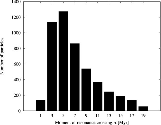
The same as in Fig. 7 but for 4937 particles that crossed the resonance without having close approach to the planets.
Interestingly, the two distributions of objects that crossed the resonance are almost identical. Moreover, it is also important to note that most of the particles crossed the resonance during the first 8 Myr, with a maximum occurring between 4 and 6 Myr. Later on, the percentage of objects that crossed the resonance increases in both figures to 100 per cent.
These results immediately suggest that many (if not most) of the objects are able to cross the 7/2 resonance if Yarkovsky force is considered.
To further evaluate the ability of asteroids to cross this resonance, we analyse how the number of objects that crossed the resonance depends on the Yarkovsky drift speed. These results are shown in Fig. 9. For this analysis, only objects without having close approach to the planets are considered.
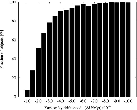
Fraction of objects that crossed the resonance as a function of Yarkovsky drift speed. Only those particles without having close approach to the planets are shown.
Unexpectedly, almost 100 per cent test particles with values of Yarkovsky drift speed higher than −5.0 × 10⁻⁴ au Myr−1 successfully crossed the resonance. As mentioned above, at heliocentric distances of the Phocaea asteroids, and assuming the S-spectral type, this corresponds to a maximum drift of an object of roughly 600 m in diameter. Our results suggest that many of the objects of this size, or smaller, should be able to cross the resonance. Thus, many of them should be found on the left side of the 7/2 resonance in terms of semimajor axis, i.e. closer to the Sun.
3.2.2 Results obtained using the second method
The results of this analysis are shown in Figs 10 and 11. As can be seen in Fig. 10, the fraction of removed bodies gradually increases for increasing da/dt, until the Yarkovsky drift speed reaches a value of −5.0 × 10⁻⁴ au Myr−1, for which 22 per cent of our simulated objects were lost during the 20 Myr integration time. For higher values of the Yarkovsky drift, the fraction of removed bodies suddenly drops to only 8 per cent and remains fairly constant also for higher values of da/dt. This behaviour is actually what we should expect. Starting from da/dt = 0 and gradually increasing this value, more and more bodies are led to interact with the 7/2 MMR. At some point (for da/dt ≳ −5.0× 10⁻⁴ au Myr−1), the semimajor axis drift becomes rapid enough to allow many bodies to cross the resonance in a time sufficiently short to prevent resonant mechanism to efficiently pump up eccentricity to the point of allowing close encounters with Mars. In this way, fast moving objects have better chances to survive resonance crossing. As was explained above, a drift rate higher than −5.0 × 10⁻⁴ au Myr−1 should apply to the cases of S-class asteroids smaller than 0.6 km in diameter, in the Phocaea region.
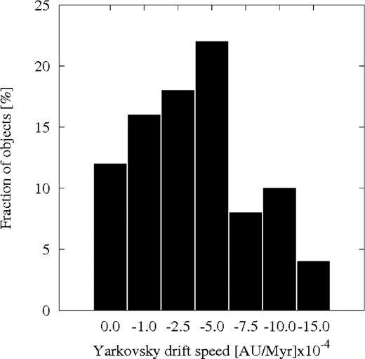
The fraction of removed asteroids during a 20 Myr numerical integration versus the assumed da/dt drift speed due to the Yarkovsky thermal force.
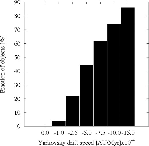
The fraction of asteroids that successfully cross the 7/2 MMR during our 20 Myr numerical integration as a function of the assumed da/dt drift speed caused by the Yarkovsky thermal force.
In Fig. 11, we show the fraction of bodies that cross the 7/2 resonance for different values of da/dt. This result shows that a significant fraction of the bodies larger than about 0.6 km should be able to cross the resonance.
In comparison with the results obtained by applying the first method, here we found the size limit at which most of the objects should be able to cross the 7/2 resonance to be shifted to slightly smaller sizes. Still, the results obtained by two methods are in agreement and undoubtedly yield the same conclusions.
4 SUMMARY AND CONCLUSIONS
Results obtained in this work, using two similar but still different methods, suggest that if the highest estimated Yarkovsky drift speed is assumed, most of the bodies smaller than about 600 m in diameter can transit across the 7/2 resonance without being removed from the Phocaea region. In any case, it seems that despite being effective in pumping up asteroid eccentricities in this region, the 7/2 resonance is not an absolute dynamical boundary for sufficiently small objects, below some hundred metres in diameter.
However, as discussed before, and as could be seen in Fig. 12, there is an important drop in the number density of asteroids on the left side of the resonance, in terms of semimajor axis. So, how could this be explained?
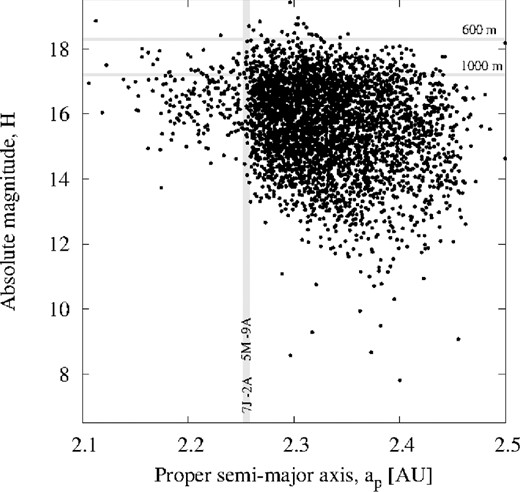
The distribution of the Phocaea asteroids shown in the ap–H plane. The vertical dashed area marks the position of two MMRs, namely the 7/2 with Jupiter and 5/9 with Mars.
Based on the results obtained here, we propose the following explanations. First, the observed comparative paucity of bodies at semimajor axes smaller than 2.256 au for absolute magnitudes above H = 18 is simply a consequence of the present observational completeness limit. Interestingly, this limit in the Phocaea region should be around diameter of 0.6–0.7 km, just above the limit at which most of the asteroids should be able to transit across the resonance according to our results. Thus, it is possible that many of these small asteroids do exist, but they are still waiting to be discovered.
Moreover, in practice, the Yarkovsky thermal force depends on many parameters including the orientation of the spin axis, period of rotation, etc. Besides, we did not consider here Yarkovsky–O'Keefe–Radzievsky–Paddack effect nor other possible mechanisms that may change the asteroid spin axis orientation (e.g. non-destructive collisions). These effects in general reduce the efficiency of the Yarkovsky effect (Vokrouhlický et al. 2006). The above-inferred size limit is obtained assuming that the fastest possible Yarkovsky-induced drift is maintained over the whole interval covered by the integrations. Thus, the real size limit is likely shifted a bit towards smaller values.
Finally, the lack of asteroids at a < 2.256 au is probably at least partly a consequence of the dynamical instabilities in this region. These instabilities are mainly caused by the inner planets as shown by Morbidelli & Nesvorny (1999). A slow Yarkovsky-driven drift in orbital semimajor axis for bodies larger than some hundreds of metres can lead to removal of these bodies when they reach the 7/2 MMR with Jupiter or the 5/9 MMR with Mars. We have seen that the semimajor axis drift of smaller objects should be sufficiently fast to allow them to transit safely across powerful resonances, so that lower-than-expected observed population in the interval 2.1–2.25 au is likely due to significant leakage.
Thus, our results seem to be in very good agreement with the currently available observational data. Still, for a definite confirmation we need to wait until the completeness limit reaches the sizes at which our results predict that most of asteroids should transit across the 7/2 resonance. At these sizes, the sharp drop of the number density should disappear. As the number of new asteroids grows quickly, these should be testable in the near future.
We would like to thank Valerio Carruba, the referee, for his useful suggestions which helped to improve this paper. This work has been supported by the Ministry of Education, Science and Technological Development of the Republic of Serbia, under the Project 176011. BN also acknowledges support by the European Union [FP7/2007-2013], project: STARDUST-The Asteroid and Space Debris Network.
The g and s are the average rates of the longitude of perihelion ϖ and of the longitude of node Ω, respectively. The indices from 2 to 7 refer to planets from Venus to Uranus, respectively.
Note that there is also an alternative notation of non-linear SRs. In this notation, instead of using explicitly proper frequencies, a kind of condensed notation is utilized (see e.g. Carruba 2009). For example, the g − g6 − s + s6 resonance may be denoted as ν6 − ν16. Analogously, the s − s4 + g3 − g7 becomes the ν7 − ν3 + ν14 resonance.
Available from http://adams.dm.unipi.it/orbfit/
In principle, the outcome of resonance crossing may depend on the value of the resonant angle at which the test particle enters the resonance, and different values of this angle may produce different results. However, as we are using here a large sample of test particles, random choice of angles seems to be appropriate.
