


Abstract
We present deep 10 h VLT/XSHOOTER spectroscopy for an extraordinarily luminous and extended Ly α emitter at z = 6.595 referred to as Himiko and first discussed by Ouchi et al., with the purpose of constraining the mechanisms powering its strong emission. Complementary to the spectrum, we discuss near-infrared imaging data from the CANDELS survey. We find neither for He II nor any metal line a significant excess, with 3σ upper limits of 6.8, 3.1, and 5.8 × 10⁻¹⁸ erg s−1 cm−2 for C IV λ1549, He II λ1640, C III] λ1909, respectively, assuming apertures with 200 km s−1 widths and offset by −250 km s−1 w.r.t. to the peak Ly α redshift. These limits provide strong evidence that an AGN is not a major contribution to Himiko's Ly α flux. Strong conclusions about the presence of Pop III star formation or gravitational cooling radiation are not possible based on the obtained He II upper limit. Our Ly α spectrum confirms both spatial extent and flux (8.8 ± 0.5 × 10⁻¹⁷ erg s−1 cm−2) of previous measurements. In addition, we can unambiguously exclude any remaining chance of it being a lower redshift interloper by significantly detecting a continuum redwards of Ly α, while being undetected bluewards.
1 INTRODUCTION
An increasingly large number of galaxies is found by their Lyman α (Ly α) emission in narrow-band imaging surveys at redshifts up to z ∼ 7.3 (e.g. Ouchi et al. 2010; Shibuya et al. 2012).1 Searches are ongoing to find Ly α emitters (LAEs) at redshifts z ∼ 7.7 and 8.8 (e.g. Clément et al. 2012; McCracken et al. 2012; Milvang-Jensen et al. 2013), but first results beyond z ∼ 7 indicate a rapid decline in the fraction of star-forming galaxies with strong observable Ly α emission (e.g. Konno et al. 2014). This is in agreement with the low number of Ly α detections in spectroscopic follow-ups for Lyman-break-selected galaxies (e.g. Stark et al. 2010; Caruana et al. 2012, 2014; Treu et al. 2013; Pentericci et al. 2014). Such an evolution can be caused either by an increased amount of neutral hydrogen in the vicinity of the galaxies or by a change in galaxy properties, e.g. in the escape of the ionizing continuum (e.g. Dijkstra et al. 2014).
Typical LAEs at redshift z ∼ 2–3 are compact and faint (e.g. Nilsson et al. 2007; Grove et al. 2009), but a population of LAEs with emission extending up to 100 kpc has been found (e.g. Fynbo, Møller & Warren 1999; Steidel et al. 2000; Francis et al. 2001; Nilsson et al. 2006). Currently the most distant object showing characteristics of a Ly α blob (LAB), despite the effects of cosmological surface brightness dimming, is the source Himiko found by Ouchi et al. (2009) at a redshift of 6.6 with Subaru/NB921 imaging.
While low surface brightness extended Ly α haloes are identified to be a generic property around LAEs (e.g. Steidel et al. 2011; Matsuda et al. 2012), several mechanisms are theoretically proposed to support the much stronger extended Ly α emission of LABs. Each of them might be responsible either alone or in combination. The suggested possibilities include cooling emission from gravitationally inflowing gas (e.g. Haiman, Spaans & Quataert 2000; Dekel et al. 2009; Dijkstra & Loeb 2009; Scarlata et al. 2009; Faucher-Giguère et al. 2010), superwinds produced by multiple consecutive supernovae (SNe; e.g. Taniguchi & Shioya 2000), photoionization by AGNs (e.g. Haiman & Rees 2001), extreme starbursts in the largest overdensities, where the individual galaxies in the protocluster are jointly contributing to make up a blob (Cen & Zheng 2013), and starbursts within major mergers (Yajima, Li & Zhu 2013).
Observational evidence from individual objects suggests that several of these mechanisms may contribute. Hayes, Scarlata & Siana (2011) find based on polarization measurements evidence for Ly α photons to be originating from a central source and being scattered at the surrounding neutral hydrogen. In other cases, evidence for an AGN as a central ionization source is found directly (e.g. Kurk et al. 2000; Bunker et al. 2003; Weidinger, Møller & Fynbo 2004). In a few cases, due to the absence of an apparent central ionizing source (starburst or AGN) it has been argued for gravitational cooling radiation as the only remaining scenario (Nilsson et al. 2006; Smith & Jarvis 2007). However, this is a conclusion which can be challenged (Prescott et al. 2015) as haloes producing the required amount of cooling radiation would be expected to have a star-forming galaxy at their centre. Prescott et al. (2015) have found a possible ionizing source for the Nilsson et al. (2006) object in a hidden AGN offset from peak Ly α emission.
Substantial observational efforts have already been devoted to Himiko (e.g. Ouchi et al. 2009, 2013; Wagg & Kanekar 2012). In this paper, we present deep VLT/XSHOOTER (Vernet et al. 2011) spectroscopy of this remarkable object, extending over the full range from the optical to the near-infrared (NIR) H band. The main purpose of the observation is to search for other emission lines than Ly α, which helps to shed further light on the origin of the extended Ly α emission. In particular, both a very hot stellar population (e.g. Schaerer 2002; Raiter, Schaerer & Fosbury 2010), as expected for a metal-free Population III (Pop III), and gravitational cooling radiation (e.g. Yang et al. 2006) would give rise to relatively strong He II λ1640 emission. By contrast, due to preceding metal-enrichment, an AGN is expected to display in addition to He II high-ionization emission lines from C, Si or N. We supplement the spectroscopic data by analysing CANDELS JF125W and HF160W archival imaging (Grogin et al. 2011; Koekemoer et al. 2011).
In Section 2.1, we describe our spectroscopic observations, while we give details about the data reduction in Section 2.2, followed by a discussion of the photometry done on archival data (Section 2.3). Results for the Ly α spatial distribution, the spectral rest-frame UV continuum, Ly α flux and profile, and non-detection limits for the rest-frame far-UV lines are presented in Sections 3.1 through 3.4. Subsequently, we discuss in Sections 4.1 and 4.2 implications from the broad-band spectral energy distribution (SED), in Section 4.3 a possible interpretation of the Ly α shape, and finally and most important in Section 4.4 the implications from our non-detection limits for the mechanisms powering Himiko.
Throughout the paper, a standard cosmology (ΩΛ, 0 = 0.7, Ωm, 0 = 0.3, H0 = 70 km s−1) was assumed. All stated magnitudes are on the AB system (Oke 1974). Unless otherwise noted, all wavelengths are converted to vacuum wavelengths and corrected to the heliocentric standard. A size of 1 arcsec corresponds at z = 6.595 to a proper distance of 5.4 kpc. The Universe was at that redshift 800 Myr young. When stating in the following ‘He II’, ‘C IV’, ‘C III]’, and ‘N V’, we are referring to He II λ1640, C IV λλ1548, 1551, [C III]C III] λλ1907, 1909, and N V λλ1239, 1243, respectively.
2 DATA
2.1 Spectroscopic observations
The XSHOOTER data have been taken at VLT-UT2 (Kueyen) in the second half of the nights starting on 2011 September 2, 3, and 4, subdivided into nine different observing blocks (OBs) with integration and observing times summarized in Table 1. We used the same set of slits for XSHOOTER's three spectral arms throughout: 1.6 arcsec × 11 arcsec (UVB), 1.5 arcsec × 11 arcsec (VIS), and 0.9 arcsec × 11 arcsec JH (NIR), which is a slit including a filter blocking wavelengths longer than 2.1 μm, effectively reducing the impact of scattered light in the NIR spectra. All used data were taken under atmospheric conditions classified as either thin cirrus (TN) or clear (CL). After excluding OB1 for being affected by thick clouds, the total usable exposure time was 35 480 s. In our NIR reduction, we used only frames with the same exposure time of 600 s, resulting in a slightly smaller total time of 33 600 s.
Number of exposures and exposure times per OB are listed. Except in OB1 and OB9, exposures were taken with 1200 s both in the VIS and UVB arm. In the NIR, each of the exposures was split into two sub-integrations with half the exposure time (e.g. 1200 s VIS ⇒ 2×600 s NIR). Where not all exposures could be used for the reduction due to passing clouds, both the used and the total number are stated. Numbers in square brackets indicate the exposure times included in the NIR stack, if different from the VIS stack.
| Date | Obs. block | # VIS exp. | Exp. time (s) | conditionsa |
|---|---|---|---|---|
| 02-09 | OB_H_1-1 | 0/1 | 0/1169.7 | TK |
| OB_H_1-2 | 4 | 4800 | TN/CL | |
| OB_H_1-3 | 2 | 2400 | TN | |
| Summary 02.09: | 6/7 | 7200/8369.7 | ||
| 03-09 | OB_H_1-6 | 4 | 4800 | TN b |
| OB_H_1-8 | 4 | 4800 | TN | |
| OB_H_1-9 | 2 | [0] 1880 c | CL | |
| Summary 03.09: | 10/10 | [9600] 11 480/11 480 | ||
| 04-09 | OB_H_1-10 | 6 | 7200 | CL |
| OB_H_1-11 | 6 | 7200 | CL | |
| OB_H_1-12 | 2 | 2400 | CL | |
| Summary 04.09: | 14 | 16 800 | ||
| Complete summary: | 30/31 | [33 600]35 480 ([9.3]9.9 h) |
aCL: clear, TN: thin cirrus, TK: thick cirrus bTK E @40°. cTwo exposures were taken with 940 s (VIS) and 2×470 s (NIR). For the NIR reduction, we did not use the 470 s exposures.
Acquisition on our target's narrow-band image (NB921; Ouchi et al. 2008, 2009) centroid in the slit's centre was obtained through a blind offset from a star located 48.14 arcsec west and 8.99 arcsec north. We can claim that the pointing accuracy, at least along the slit, was in each of the OBs better than 0.1 arcsec, as can be concluded from the spatial centroid of Ly α in each of the OBs (cf. Table 2). As the NIR spectrum is observed in XSHOOTER simultaneously with Ly α in the VIS arm, we can exclude the possibility of non-detections due to pointing problems.
Results of a Gaussian fit to the spatial Ly α profiles as measured in the individual OBs (cf. Fig. 5) and the stacked spectrum. The ‘centre’ column gives the displacement w.r.t to the expected position. In addition, the seeing of the individual OBs, corrected to observed wavelength and airmass, is stated.
| OB | Centre | FWHM (fit) | Seeing | fLy α |
|---|---|---|---|---|
| 10−17 | ||||
| arcsec (slit) | arcsec (slit) | arcsec | erg s−1 cm−2 | |
| OB 2 | −0.01 ± 0.04 | 1.24 ± 0.08 | 0.6 | 6.1 ± 0.5 |
| OB 3 | −0.14 ± 0.07 | 1.43 ± 0.16 | 0.6 | 6.4 ± 0.6 |
| OB 6 | −0.07 ± 0.04 | 1.25 ± 0.10 | 0.8 | 6.1 ± 0.5 |
| OB 8 | −0.03 ± 0.05 | 1.23 ± 0.12 | 0.6 | 5.6 ± 0.4 |
| OB 9 | −0.03 ± 0.08 | 1.51 ± 0.20 | 0.6 | 6.5 ± 0.8 |
| OB 10 | −0.08 ± 0.04 | 1.60 ± 0.08 | 0.8 | 6.2 ± 0.4 |
| OB 11 | −0.05 ± 0.02 | 1.26 ± 0.06 | 0.6 | 6.2 ± 0.4 |
| OB 12 | −0.01 ± 0.05 | 1.20 ± 0.11 | 0.6 | 6.2 ± 0.6 |
| All OBs | −0.02 ± 0.02 | 1.32 ± 0.04 | 0.7 | 6.1 ± 0.2 |
Spectra were taken with a nod throw of 5.0 arcsec and a jitter box size of 0.5 arcsec, allowing for an optimal skyline removal. In order to minimize the slit loss, the position angle was set to the parallactic angle at the start of each OB. This is mainly relevant in the NIR, as the VIS and UVB arms are equipped with atmospheric dispersion correctors. The corresponding position angles are shown in Fig. 1.
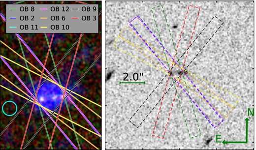
Alignment of the slit in the different OBs w.r.t to Himiko. A 5.7 arcsec × 8.3 arcsec colour composite including CANDELS WFC3 HF160W and JF125W as red and green channels, respectively, and the NB921 image as blue channel is shown in the left-hand panel. NB921 is a ground-based image with a seeing indicated by the 0.8 arcsec diameter cyan circle. The 1.5 arcsec ×11 arcsec slit, as used in the VIS arm, is included with the different orientations used during the observation. In the right, the 0.9 arcsec ×11 arcsec slits, which were used in the NIR arm, are overplotted on a 12.1 arcsec × 12.1 arcsec JF125W cutout. The legend lists the OBs in counterclockwise order (along columns). The positive slit direction is in all OBs towards the bottom of the figure, so mainly towards the south. OB11 and OB12 cannot be separated in the plot, as exactly the same position angles were used.
Assuming that emission lines are co-aligned with one or all of the three continuum bright sources, our decision to use the parallactic angle might have resulted in a higher than necessary slit loss. This can be seen from Fig. 1 (right). At the time of the observations no HST/WFC3 data were available.
It is not possible to measure the seeing directly from the Ly α spectrum, both due to resonant effects of Ly α and as Himiko is not a point source. Therefore, we needed to extract information about the seeing from the FITS header, which has an uncertainty of about 0.2 arcsec.2 Corrected to both airmass of the observations and the observed wavelength of Ly α and averaged over sub-integrations, we estimate a seeing in the individual OBs between 0.6 and 0.8 arcsec (FWHM; Table 2), with a mean value of 0.7 arcsec for the stacked OBs, or 0.6 arcsec corrected to the wavelength expected for He II wavelength.
2.2 Data reduction
We performed our final reduction using XSHOOTER pipeline version 2.3.0 (Modigliani et al. 2010), where we made a small modification to the pipeline code. This was to additionally mask all pixels neighbouring those pixels identified by the pipeline as cosmic ray hits. Without this precaution, artefacts remain in the data, which are not indicated in the pipeline quality map. Otherwise, we used mainly standard parameters.
The echelle spectra were rectified to a pixel size of 0.4 Å and 1 Å in wavelength direction and 0.16 arcsec and 0.21 arcsec in slit direction for VIS and NIR arm, respectively. We are only making use of the spectra from XSHOOTER's VIS and NIR arm, as the wavelength range covered by the UVB arm does not contain any information for this object.
While we obtained our final NIR reduction by automatically combining all frames with the pipeline using the nodding recipe,3 we could improve the result in the VIS reduction somewhat by using our own script. In the latter case, we first reduced the VIS frames in nodding pairs with the pipeline, and then combined the frames based on a weighted mean, using the inverse square of the noise maps produced by the pipeline as weights.
A nodding reduction is commonly considered as essential for a good skyline subtraction in the NIR. Nevertheless, we tried also a stare reduction both in the VIS and the NIR, which could give in an idealized case a |$\sqrt{2}$| lower noise. In the case of the NIR spectrum, where the use of dark frames taken with the same exposure time as the science frames is necessary for a stare reduction, we used a large enough number of dark frames to not be limited by their noise.4
While the stare reduction worked for the VIS arm, we experienced in the deep NIR stack spatially abruptly changing residual structures, which we could not safely remove by modelling with slowly changing functions. Consequently, we had to decide that a safe stare reduction was not feasible at this point.
By contrast, the pixel to pixel noise decreases as expected with the square root of the number of exposures in the case of the nodding reduction, as shown in Fig. 2 for a region around the expected He II line and using only pixels not affected by skylines and bad pixels. Reassuringly, this indicates that the structure seen in the stare reduction is at least within the individual nodding sequences temporarily stable and therefore removed by the nodding procedure. As the relevant VIS arm wavelength range redwards of Ly α is affected by telluric emission lines, which requires a robust sky subtraction, we decided finally to use a nodding reduction in the VIS arm, too.
In addition to those pixels flagged as bad in the pipeline, we masked skylines, which we automatically identified by iterative sigma clipping against emission in a stare reduced and non-background subtracted spectrum, and pixels with unexpected high noise, defined as having absolute counts larger than 10 times the 1σ error. Except in the region of Ly α, where we did not mask these outliers, this assumption is safe in not clipping away any source signal. Additionally, when determining the signal-to-noise (S/N) within extraction boxes over a certain wavelength region, we excluded those parts of the spectrum with a noise either 1.5 times or 2.0 times larger than the minimal noise within 200 Å of the region's centre. The decision between 1.5 and 2.0 was made based on the amount of pixels remaining for the analysis.
Comparing the calculated pixel to pixel noise to the prediction from the pipeline's noise model, we find for the stack of all 56 NIR frames an rms noise of 1.2 × 10⁻¹⁹ erg s−1 cm−2 Å−1 per pixel, while the direct pixel to pixel variations have a standard deviation of 8.1 × 10⁻²⁰ erg s−1 cm−2 Å−1. As we are using the error spectra based on the pipeline throughout this paper, stated uncertainties for several quantities might be overestimates. On the other hand, there is a correlation in the spectrum due to the rectification, which is difficult to quantify, especially as it varies with the position in the spectrum. A full characterization of the noise would require the propagation of the covariance matrix (e.g. Horrobin et al. 2008), which is currently not available in the pipeline.
The instrumental resolution at the position of Ly α and He II was determined based on fitting Gaussians to nearby skylines. We get in the two cases R = 5300 (56 km s−1) and R = 5500 (55 km s−1), respectively.
For the determination of the response function, we used a nodding observation of the standard star Feige110 taken with 5 arcsec slits during the night starting on 2011 September 3, directly before beginning with the observation of OB_Himiko_1-6. We used this response function for all OBs taken within the three nights. In the pipeline, the response function is obtained by doing a cubic spline interpolation through knots at wavelengths having atmospheric transmission close to 100 per cent. For ensuring a very good response function close to Ly α, we had to remove a knot from the default list at 9270 Å and add instead another one at 9040 Å.
In order to avoid possible issues of temporal variability of the NIR flat-field illumination, we decided to use the same flat-field observations both for the standard star and the science frame observations, even though they were taken with different slits.5 Stability and accuracy of the response function were tested by calibrating an observation of the flux standard LTT7987, taken in the second night of our programme, based on the response function determined from Feige110 in the first night. The result of this test is shown in Fig. 3 .6 We can conclude that the accuracy of the spectrophotometry is about 5 per cent.
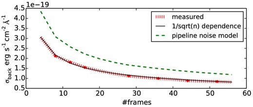
Pixel to pixel noise in skyline free regions close to the expected wavelength of He II in the NIR arm. We have successively added four frames corresponding to two nodding positions to the stack and calculated the κ − σ (κ = 4) clipped standard deviation for each of the steps. The result is the solid line. The dotted line shows the noise level as expected from a |$1/\sqrt{N}$| dependence based on the noise in the first step (four frames). It is perfectly in agreement with the data. In addition, the noise prediction from the pipeline noise model is included.
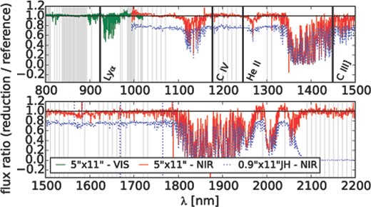
Accuracy of flux calibration based on cross-calibrating the spectrophotometric standard LTT7987, taken on September 4, against the response function from our main standard Feige110, taken on the night before. The shown curve gives the ratio between the measured LTT7987 flux and its expectation. In the NIR, results are included both for an observation using the same 5 arcsec × 11 arcsec slit for LTT7987 and FEIGE110 and for and observation of LTT7987 with the 0.9 arcsec ×11 arcsec JH slit. Thin vertical lines indicate wavelengths used by the pipeline for fitting a spline to the standard star in the response function calculation.
In order to reach the maximum possible depth for our science frames, we mainly avoided spending time on telluric standards. Only in the beginning of the observations in the first night we took one telluric standard with the same slit set-up as chosen for our science observations. We used this frame to fit a model telluric spectrum with ESO's molecfit package (Smette et al. 2015), using the input parameters suggested in Kausch et al. (2015). Based on the obtained atmospheric parameters, we created model telluric spectra for the airmass of each individual nodding pair. Here, we need to make the strong assumption of constant atmosphere over a time-scale of several hours, which is unlikely completely correct. Nevertheless, the obtained accuracy is appropriate for our purpose. For the second and third night, we used telluric standards taken for other programmes right before the start of our observations to fit the atmospheric parameters. While these observations were based on differing slits, we could use the wavelength solution and line kernel obtained for night one to create appropriate telluric spectra for nights two and three. We adjusted the error spectra after applying telluric corrections.
All 1D spectra were extracted from the rectified 2D frames. As there is no detectable trace in the NIR spectrum, we needed to assess the accuracy of the position of the trace in the rectified frame based on a check on the reduced standard star. We find that the centre of the trace does not differ more than one pixel in slit direction from the expected position over the complete range of the NIR arm.
2.3 Photometry on archival data
As located in the Subaru/XMM–Newton deep field, Himiko is covered both by very deep ground- and space-based imaging, from X-ray to radio, including the NB921/Subaru narrow-band image, which allowed Ouchi et al. (2009) to identify Himiko as a giant Ly α emitter.
Deep HST imaging is available from the CANDELS survey (Grogin et al. 2011; Koekemoer et al. 2011). This includes data from ACS/WFC in VF606W and IF814W and in JF125W and HF160W with WFC3. We performed in this work photometry on the CANDELS data.
It is noteworthy, that recently, both Jiang et al. (2013) and Ouchi et al. (2013) have published photometry in JF125W and HF160W based on two other observations (HST GO programmes 11149, 12329, 12616, and GO 12265, respectively), supplemented by deep IRAC 1 and 2 data from Spitzer/IRAC SEDS (Ashby et al. 2013). Especially the analysis of Ouchi et al. (2013) has been targeted at studying Himiko, including additional WFC3/F098M intermediate band data which allowed them to identify peaks in the Ly α distribution and ALMA [C II] observations.
Ground-based NIR data in J, H, and K is available from the ultradeep component (UDS) of the UKIRT Infrared Deep Sky Survey (UKIDSS; Lawrence et al. 2007). We are using the UKIDSS data release 8 (UKIDSSDR8PLUS), which has significantly increased depth compared to previous releases.7
For our SED fitting in Section 4.1, we are using NIR photometry determined by us from the CANDELS and the UKIDSS data and supplement it by the IRAC SEDS (1 and 2) and IRAC SpUDS (3 and 4) (Dunlop et al. 2007) photometry presented by Ouchi et al. (2013).
We determined magnitudes in several apertures on all optical and NIR images with SExtractor's double image mode (Bertin & Arnouts 1996), with CANDELS JF125W as detection image. Without unwanted resampling, it is due to the requirement of the same pixel scale in double mode not directly possible to use JF125W as detection image for all other images. Therefore, we put fake-sources in images with the appropriate pixel scale at the positions determined from the JF125W image and used these as input in double mode. As the UKIDSS photometric system is in VEGA magnitudes, we use the VEGA to AB magnitude corrections of 0.938, 1.379, 1.900 as stated in Hewett et al. (2006) for J, H, and K, respectively.
Consistent with the visual impression (Fig. 1), we detect in the JF125W image three distinct sources at the position of Himiko. We refer in the following to these sources as Himiko–E (east), Himiko–C (centre), Himiko–W (west). Their coordinates are stated in Table 3. The transverse distance between Himiko–E and Himiko–W is 1.18 arcsec (6.4 kpc), while the distance between Himiko–C and Himiko–W is 0.46 arcsec (2.5 kpc).
Magnitudes in 0.4 arcsec diameter apertures on the CANDELS HST images are stated for the three distinct continuum sources identified with Himiko (cf. Fig. 1). No aperture corrections are applied. The stated UV slope β (fλ ∝ λβ) is based on the estimator β = 4.43(JF125W − HF160W) − 2 (Dunlop et al. 2012). Upper limits are 1σ values.
| Himiko–E | Himiko–C | Himiko–W | |
|---|---|---|---|
| R.A. | |$+2^{\rm h}17^{\rm m}57 {.\!\!\!\!^{{\mathrm{s}}}}612$| | |$+2^{\rm h}17^{\rm m}57 {.\!\!\!\!^{{\mathrm{s}}}}564$| | |$+2^h17^{\rm m}57 {.\!\!\!\!^{{\mathrm{s}}}}533$| |
| Dec | −5°08′44|${^{\prime\prime}_{.}}$|90 | −5°08′44|${^{\prime\prime}_{.}}$|83 | −5°08′44|${^{\prime\prime}_{.}}$|80 |
| VF606W | >29.53 | >29.53 | >29.53 |
| IF814W | 28.45 ± 0.64 | >29.02 | 28.52 ± 0.68 |
| JF125W | 26.47 ± 0.07 | 26.66 ± 0.10 | 26.53 ± 0.09 |
| HF160W | 26.77 ± 0.12 | 26.97 ± 0.15 | 26.49 ± 0.10 |
| J − H | −0.30 ± 0.14 | −0.31 ± 0.18 | 0.04 ± 0.13 |
| β | −3.33 ± 0.62 | −3.37 ± 0.80 | −1.82 ± 0.60 |
In order to obtain accurate error estimates for the fluxes measured within circular apertures,8 we determined several measurements with apertures of the same size as used for the object in non-overlapping source free places. For images exhibiting correlated noise, as being the case for the drizzled or resampled mosaic images used for our analysis, this is the appropriate way to account for the correlation. From the κ-σ clipped standard deviation of these empty-aperture measurements, we obtained the 1σ background limiting flux in the chosen aperture. The clipping with a κ = 2.5 and 30 iterations makes sure that apertures including strong outlying pixels or which despite the method to find source free places are not really source free are rejected.
We defined source free regions based on the SExtractor segmentation maps and masking of obvious artefacts like spikes or blooming. In addition, we made sure that the used regions have approximately the same depth as the region including Himiko. Depending on the available area, we had for the different images between 26 and 190 non-overlapping empty apertures.
In Table 3, measurements within 0.4 arcsec diameter apertures centred on each of the three peaks are listed for the HST images, while magnitudes within 2.0 arcsec apertures are stated for all used images in Table 4. In the latter case, the apertures are centred on the same position as that stated in Ouchi et al. (2009, 2013). In addition, aperture corrected magnitudes are included. To calculate the appropriate aperture corrections for the images with larger point spread functions (PSFs), we assumed that in all the considered bands the flux is coming from the three main sources and that the flux ratio between the three peaks is the same as in the JF125WHST image. This allows us to convolve this flux distribution with the PSF9 and consequently determine the fraction of the total flux included in the aperture on the created fake image by using SExtractor in the same way as for the science measurements. For the PSF profiles, we assumed in the case of the UKIRT/WFCAM NIR images Gaussians determined by a fit to nearby stars. We get for J,H,K FWHMs of 0.74, 0.74, and 0.69 arcsec, respectively.
Magnitudes as measured in 2 arcsec apertures for the CANDELS/HST and the UKIDSS/UDS data. In addition the Spitzer/IRAC measurements from Ouchi et al. (2013) are included. First and second column list measurements without aperture correction and the corresponding 1σ errors. Magnitudes after applying aperture corrections are stated in the third column. Upper limits are 1σ values. β is calculated as in Table. 3.
| Filter | Mag (2 arcsec) | σ Mag (2 arcsec) | Total magnitude |
|---|---|---|---|
| VF606W | >27.47 | – | >27.47 |
| IF814W | >26.77 | – | >26.78 |
| JF125W | 24.71 | 0.13 | 24.71 |
| J | 25.23 | 0.26 | 25.09 |
| HF160W | 24.93 | 0.15 | 24.93 |
| H | >25.59 | – | >25.44 |
| K | 24.84 | 0.22 | 24.72 |
| 3.6 μm a | – | 0.09 | 23.69 |
| 4.5 μm a | – | 0.19 | 24.28 |
| 5.8 μm a | – | – | >23.19 |
| 8.0 μm a | – | – | >23.00 |
| β | −3.0 ± 0.9 |
aMeasurements taken from Ouchi et al. (2013).
Finally, Tables 3 and 4 also include the UV slope β (fλ ∝ λβ). We calculated it based on the estimator β = 4.43(JF125W − HF160W) − 2 (Dunlop et al. 2012). Both the total object and the two eastern components seem to have very steep slopes of −3.0 ± 0.9, −3.3 ± 0.6, −3.4 ± 0.8, respectively. However, the uncertainties are large.
Interestingly, there seems to exist a slight tension between the JF125W in the data used by us (CANDELS) and that obtained by Ouchi et al. (2013) with 24.71 ± 0.13 and 24.99 ± 0.08, respectively. This corresponds to a difference of about 1.8σ. Consequently, they infer a less steep slope of β = −2.00 ± 0.57. While Jiang et al. (2013) have not derived magnitudes for the three individual sources, their total magnitude is with 24.61 ± 0.08 deviating even more. However, they have been using SExtractorMAG-AUTO measurements. Therefore, the comparison between their values and those derived by Ouchi et al. (2013) and us should be treated with caution. On the other hand, the ground-based UKIDSS J magnitude is with 25.09 ± 0.26 closer to the value obtained by Ouchi et al. (2013).
The greatest difference between the CANDELS data and that from Ouchi et al. (2013) is in the central component. They measure from their data 27.03 ± 0.07 for JF125W and we derive 26.66 ± 0.10. A subjective visual inspection of the Jiang et al. (2013) data seems to rather confirm the relatively blue colour in the central blob.
For all stated coordinates, we use the world coordinate system as defined in the CANDELS JF125W image (J2000). We find that this coordinate system is slightly offset w.r.t to the coordinate system used by Ouchi et al. (2009). Their coordinate10 corresponds to RA, DEC = |$+2^{\rm h}17^{\rm m}57 {.\!\!\!\!^{{\mathrm{s}}}}581$|, −5°08′44|${^{\prime\prime}_{.}}$|72 in the CANDELS JF125W astrometric system. The UKIDSS data appears within the uncertainties well matched to the CANDELS astrometry. Therefore, we do not apply any correction here. Fig. 1 (left) includes an R,G,B composite using HF160W, JF125W (both CANDELS), and NB921, respectively. Cutouts around the position of Himiko for all used images are shown in Fig. 4.
Images in following filters in the stated order: VF606W, IF814W, NB921, JF125W, HF160W, UKIDSS/UDS K. The images are scaled for optimal viewing from −3 × σ to 1.1 × max, where σ and max are the standard deviation and maximum value of the pixels within a circular annulus around the source, respectively. Green, blue, and red circles refer to the three sources visible in the JF125W and HF125W images.
3 RESULTS
3.1 Spatial flux distribution and slit losses
The different OBs taken with different position angles allow us to compare the spatial extent of Ly α along the slit to the NB921 image for several orientations. To do so, we extracted for each OB a Ly α spatial profile averaged over the wavelength range from 9227 to 9250 Å, and replicated this for the NB921 image by assuming an aperture with the shape of the 1.5 arcsec slit and calculating a running mean over pseudo-spatial bins of 0.2 arcsec. The 0.8 arcsec FWHM (full width at half-maximum) seeing of the NB921 image (Ouchi et al. 2009) is slightly larger than that expected in the different OBs of our spectral data (cf. Table. 2), but within the uncertainties comparable.
We quantified the centroid and spatial width of Ly α in each of the individual OBs by fitting Gaussians to the spatial profiles. Resulting values and the integrated Ly α flux over the same range are stated in Table 2. The centroids imply an excellent pointing accuracy.
For comparison, the expected spatial profile for the continuum within the slit was estimated based on fake JF125W images (cf. Section 2.3), convolved with the estimated seeing for each OB. All three profiles are shown for three example OBs (2, 8, and 10) in Fig. 5.
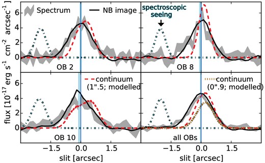
Ly α spatial profiles for three individual example OBs (2, 8, and 10) and for the complete stack of all OBs. Included are profiles directly extracted from the spectrum over the wavelength range from 9227 to 9250 Å and profiles extracted from images under the assumption of the 1.5 arcsec slit. The latter is shown both for the NB921 image and a JF125W image, which was corrected to the seeing of the individual spectroscopic OBs. Finally, for the stack the expected continuum profile is also shown for the 0.9 arcsec slit. The legend is split between the different panels, but applies to all four sub-panels.
The profiles extracted from the spectrum are as expected in good agreement with the NB921 image. For those OBs, like OB8, which are nearly perpendicular to the alignment of the three individual sources, the Ly α profile is significantly more extended than the estimated continuum profile. The main excess in the emission seems to be towards the north. On the other hand, for those OBs like OB10, with the slit aligned closer to the east–west direction, there seems to be an offset of the continuum towards the west. This indicates Ly α emission more concentrated on the eastern parts, in agreement with the F098M/WFC3 observations of Ouchi et al. (2013). We note that the conclusions would not change when assuming different seeing values within ±0.2 arcsec of the values taken from the header.
Finally, the spatial profile of the combined Ly α stack is shown in the lower-right panel of Fig. 5. The shown NB921 and continuum profiles have been calculated as the average of all contributing frames with their respective position angles. In this panel, we are showing in addition the profile for the continuum as expected in the 0.9 arcsec slit. Noteworthy, we expect the continuum offset by 0.2 arcsec towards positive slit directions w.r.t to the Ly α centroid.
Slit losses both for Ly α and the continuum and both for the 0.9 arcsec and the 1.5 arcsec slits were calculated based on the NB921 or the seeing convolved fake JF125W image by determining the flux fraction within slit-like extraction boxes. Identical to the profile determination, we treated the individual OBs separately, and simulated the stack, by combining the slit losses for the individual OBs weighted with the appropriate exposure times.
Assuming the 1.5 arcsec VIS arm slit and an extraction width of 4 arcsec along the slit, being close enough to no loss in slit-direction, results in a slit loss factor of 0.7 (0.4 mag) for Ly α based on the NB921 image.
We determined the optimal extraction-mask size for the expected continuum distribution under the assumption of background limited noise. We did so by maximizing the ratio between enclosed flux and the square root of the included pixels. The maximum value is reached in the 1.5 arcsec VIS slit between 7 and 9 pixels, when keeping the centre of the extraction mask at the formal centre of the slit. For an eight pixel (1.28 arcsec) extraction width, we derive a slit loss factor of 0.74 ± 0.09 (0.32 ± 0.13 mag). The stated uncertainties are resulting from the assumed uncertainty on the seeing.
The spatial distribution for possible He II or metal line emission is not known. Therefore, we consider hypothetically both the cases that it is co-aligned with the continuum or with the Ly α emission. Assuming the two distributions, we obtain optimal extraction widths in the 0.9 arcsec slit with around six and eight pixels (1.26 and 1.68 arcsec), respectively, fixing the trace centre at the formal pointing position in both cases. As a compromise, we assumed for the default extraction a width of seven pixels, corresponding in the continuum and the NB921 case to slit loss factors of |$0.53^{+0.10}_{-0.05}$| (|$0.7^{+0.11}_{-0.09}$| mag) and 0.4 (1.0 mag), respectively. Certainly, alternative scenarios are possible which could lead to lower or higher slit losses, e.g. if line emission would be originating mainly from the central or the westernmost source, respectively.
3.2 Spectral continuum
We made the continuum hidden in the noise of the rectified full resolution spectrum visible by strongly binning the telluric corrected 2D spectrum in wavelength direction from an initial pixel scale of 0.4 Å pixel−1, as produced with the pipeline, to a pixel scale of 11.2 Å pixel−1. Instead of taking a simple mean of the pixels contributing to the new wavelengths bins, we calculated an inverse variance weighted mean, with the variances taken from the pipeline's error-spectrum. This allows us to obtain a low-resolution spectrum with relatively high S/N in a region strongly affected by telluric emission or absorption. One caveat with this approach is that the flux is not correctly conserved for wavelength ranges where both the flux density and the noise changes quickly. This is the case at the blue side of the Ly α line (cf. Fig. 7). Therefore, we used for our binned spectrum a simple mean in the region including Ly α.
A faint continuum is clearly visible in the resulting spectrum redwards of Ly α and due to intergalactic medium (IGM) scattering not bluewards, as expected for Himiko's redshift (Fig. 6). A similar effort in the NIR did not reveal an unambiguous continuum detection.
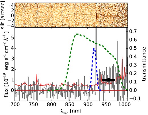
VIS spectrum telluric corrected and binned to a pixel scale of 11.2 Å pixel−1. Instead of taking a simple mean of the pixels contributing to the new wavelengths bins, we calculated a weighted mean (Section 3.2). Included are the response profiles for the Subaru NB921 and z′ filters. The trace is shown in black, while the red curve is the error on the trace. The black error bar shows the continuum level from the spectrophotometry. No heliocentric velocity correction was applied for this plot.
The detection allows us to directly determine the continuum flux density close to Ly α. For the interval from 9400 to 9750 Å (1238 to 1285 Å rest frame), chosen to be in a region with comparably low noise in our optimally rebinned spectrum, we get with the 1.28 arcsec extraction mask a flux density of 10.1 ± 1.4 × 10⁻²⁰erg s−1 cm−2 Å−1 (cf. Fig. 6). We used in the calculation a κ–σ clipping with a κ = 2.5, rejecting one spectral bin.
The determined flux density is equivalent to an observed magnitude of 25.18 ± 0.15, or after applying the aperture correction of 0.32 mag, of 24.85 ± 0.15, corresponding to a rest-frame absolute magnitude of M1262; AB = −21.99 ± 0.15. The magnitude is slightly fainter than the CANDELS JF125W measurement (24.71 ± 0.13) and slightly brighter than the HF160W magnitude (24.93 ± 0.15), but within the errors consistent with both of them.
3.3 Ly α
The final 2D VIS spectrum in the wavelength region around Ly α is shown in Fig. 7, from which we extracted the 1D Ly α spectrum. This was done in an optimal way (Horne 1986), using a Gaussian fit to the spatial profile. The resulting 1D spectrum is plotted in Fig. 8. As a sanity check, we compared this result to extractions based on simple apertures of different widths. Large enough apertures converged within the errors to the result from the optimal extraction.
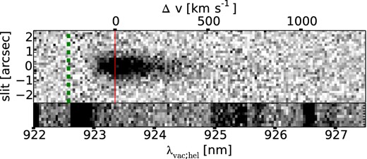
2D Ly α spectrum. The green dashed and solid red vertical lines are at the same wavelengths as in Fig. 8. Below, a non-background removed spectrum is shown for the same wavelength range, indicating positions of skylines.
![Extracted Ly α spectrum based on the stack of all OBs (solid blue). The orange dotted curve gives the errors on the flux density. Red solid and dashed green vertical lines mark the peak of the Ly α line and a velocity offset of −250 km s−1, respectively. In addition, both the median and the ±68 per cent intervals for the IGM transmission from Laursen, Sommer-Larsen & Razoumov (2011) [LA11] at this redshift are plotted. As a test (cf. Section 4.3), we have applied the median transmittance to a Gaussian and fit this model to the data, with the best-fit shown as red dashed line. The green dot-dashed curve is the Gaussian underlying the best-fit model. Finally, the magenta Gaussian in the left indicates the instrumental resolution.](https://oup.silverchair-cdn.com/oup/backfile/Content_public/Journal/mnras/451/2/10.1093/mnras/stv1019/2/m_stv1019fig8.jpeg?Expires=1750279069&Signature=ezmKxPmUl39HbwpAzkoTKxGyd34TWC2S0Ta3895gDptXf3vdrE22awoW2pPwgLAwTiOAT-~sfR~-Abb2~AFCx8qGCab~H91vRCOieJtgPpKvv3uGw3kSCc3tdDIOgwTjzfQmRDalMqPzy0syrpgx~gGZkFUcWWQsOHFOGXN-4oDbpDGz6NFq7ZcCwZsbBB6MNq4hRiuAbuDvYtuEPy-ATdlfffJKeUdEGD14F3ea2hX6ZKokb4JX0ECQG877BpACI6HCQeqXqZQk9omrOuSSsIexk2wYSzPtkvU-gIl5RgBylHfWEZFLKzQ1Oytq99Hm~1m49rmcTeJhvXwfYHUmQQ__&Key-Pair-Id=APKAIE5G5CRDK6RD3PGA)
Extracted Ly α spectrum based on the stack of all OBs (solid blue). The orange dotted curve gives the errors on the flux density. Red solid and dashed green vertical lines mark the peak of the Ly α line and a velocity offset of −250 km s−1, respectively. In addition, both the median and the ±68 per cent intervals for the IGM transmission from Laursen, Sommer-Larsen & Razoumov (2011) [LA11] at this redshift are plotted. As a test (cf. Section 4.3), we have applied the median transmittance to a Gaussian and fit this model to the data, with the best-fit shown as red dashed line. The green dot-dashed curve is the Gaussian underlying the best-fit model. Finally, the magenta Gaussian in the left indicates the instrumental resolution.
We determined several characteristic parameters of the directly measured Ly α line. All stated errors are the 68 per cent confidence intervals around the directly measured value based on 10 000 MC random realizations of the spectrum using the error spectrum. It needs to be noted that this approach overestimates the uncertainties, as the noise is added twice, once in the actual random process of the observation and once through the simulated perturbations. This means that the resulting perturbed spectra are effectively representations for a spectrum containing only half the exposure time. Yet, the values based on this simple approach allow us to get a sufficient idea of the accuracy of the determined parameters.
The pixel with the maximum flux density is at a λvac; hel of |$9233.5^{+1.2}_{-0.4}\, {A\!\!\!\!\!\!\!^{^\circ}}$| . This corresponds to a redshift of |$6.5953^{+0.0010}_{-0.0003}$|.11 The peak Ly α redshift, zpeak, is due to Ly α radiative transfer effects likely different from the systemic redshift of the ionizing source (cf. Section 4.3). For the FWHM of the line we measure |$286^{+13}_{-25}\,\mathrm{km}\,\mathrm{s}^{-1}$|. Ouchi et al. (2009) get for their Keck/DEIMOS spectrum a zpeak of 6.595 and an FWHM of 251 ± 21 km s−1, consistent with our result.
Furthermore, we calculated the skewness parameters S and Sw (Kashikawa et al. 2006). For a wavelength range from 9227 to 9250 Å, we get values of 0.69 ± 0.07 and |$12.4^{+1.4}_{-1.8}\,{A\!\!\!\!\!\!\!^{^\circ}}$| for S and Sw, respectively. This is again consistent with the result obtained by Ouchi et al. (2009): S = 0.685 ± 0.007 and Sw = 13.2 ± 0.1Å. Using an increased wavelength range from 9220 to 9260 Å, we measure values of 0.9 ± 0.2 and 16 ± 4 Å for the two quantities, being consistent with the results for the smaller range, but possibly indicating a somewhat larger value. Indeed, the spectrum might show some Ly α emission at high velocities (cf. Fig. 7). However, this is weak enough to be due to skyline residuals and we do not discuss it further.
Integrating the extracted spectrum over the wavelength range from 9227 to 9250 Å, the obtained flux is 6.1 ± 0.3 × 10⁻¹⁷ erg s−1 cm−2. After subtracting the continuum level, the Ly α flux is 5.9 ± 0.3 × 10⁻¹⁷ erg s−1 cm−2, or 8.8 ± 0.5 × 10⁻¹⁷ erg s−1 cm−2 after correcting for the slit loss factor of 0.67, as derived in Section 3.1. This corresponds to a luminosity of 4.3 ± 0.2 × 1043 erg s−1. By comparison, Ouchi et al. (2009) derive a fLy α of 7.9 ± 0.2 × 10⁻¹⁷ erg s−1 cm−2 and 11.2 ± 3.6 × 10⁻¹⁷ erg s−1 cm−2 from the z′/NB921 photometry and their slit loss corrected Magellan/IMACS spectrum, respectively. This is in good agreement with our result, considering that the slit loss as calculated from the NB921 image will only be approximately correct, as the seeing in our observation is not known with certainty (cf. Section 3.1).
From the continuum flux measured in the spectrum and the measured Ly α flux, we derive a Ly α (rest frame) equivalent width (EW0) of 65 ± 9 Å, nearly identical to the |$78^{+8}_{-6}\,{A\!\!\!\!\!\!\!^{^\circ}}$| stated by Ouchi et al. (2013). Jiang et al. (2013) have in their recent study derived a Ly α EW0 of only 22.9 Å for Himiko. The explanation for this discrepancy is that they have fitted a fixed UV slope based on their relatively blue JF125W–H160W and extrapolated this slope to the position of Ly α. However, the continuum magnitude derived from our spectrum is not consistent with this assumption.
3.4 Detection limits for rest-frame far-UV lines
As we do not unambiguously detect any of the potentially expected emission lines except Ly α, we focus on determining accurate detection limits. The instrumental resolution of 55 km s−1 allows us to resolve the considered lines for expected line widths. Therefore, detection limits depend strongly both on the line width, and, due to the large number of skylines of different strengths, on the exact systemic redshift. As the systemic redshift is not known exactly from the Ly α profile alone and the search for [C II] by Ouchi et al. (2013) resulted in a non-detection, too, all limits need to be determined over a reasonable wavelength range.
Studies to determine velocity offsets between the systemic redshift and Ly α for LAEs around z ∼ 2–3 find Ly α offsets towards the red ranging between 100 and 350 km s−1 (e.g. McLinden et al. 2011; Chonis et al. 2013; Guaita et al. 2013; Hashimoto et al. 2013), while the typical velocity offset for z ∼ 3 Lyman-break galaxies (LBGs) is with about 450 km s−1 higher (Steidel et al. 2010). On the other hand, in LABs also small negative offsets (blueshifted Ly α) have been observed (McLinden et al. 2013).
Whereas offsets at the redshifts of the aforementioned studies are produced by dynamics and properties of the interstellar (ISM) and circumgalactic medium (CGM), at the redshift of Himiko an apparent offset can also be produced by a partially neutral IGM (cf. Section 4.3).
In the case of the N V λλ1238, 1242, C IV λλ1548, 1551, and [C III], CIII] λλ1907, 1909 doublets we formally calculated values jointly in two boxes centred on the wavelengths of the two components for a given redshift. Wide extraction boxes merge into a single box. Where we state wavelengths instead of redshift or velocity offset, we refer to the central-wavelength of the expected ‘blend’. Widths are stated for the individual boxes, meaning that the effective box widths are larger.
While we test over a wide parameter space, we refer in the following several times to somewhat arbitrary fiducial detection limits based on a narrow 200 km s−1 and a wider 600 km s−1 extraction box, assuming a systemic redshift 250 km s−1 bluewards of peak Ly α, which is as mentioned above a typical value for LAEs. This redshift is also marked in several plots throughout the paper as green dashed line.
We took account for the continuum by removing an estimated continuum directly in the telluric corrected rectified 2D frame. The assumed spatial profiles in cross-dispersion direction for the 0.9 arcsec NIR and 1.5 arcsec VIS slits are those estimated from the seeing-convolved HST imaging (cf. Section 3.1). While we assumed for the region around N V λ1240 in the VIS arm a continuum with fλ(λ) = 10.2 × 10⁻²⁰ erg s−1 cm−2 Å−1, being the flux measured directly from the spectrum as described in Section 3.3 and corrected for aperture loss, we were using for the NIR spectrum a fλ(λ) = 3 × 10⁻²⁰ erg s−1 cm−2 Å−1 within the slit at the effective wavelength of HF160W and a spectral slope of β = −2.
The used NIR flux density is close to that of the measured HF160W. Due do the difference between our JF125W and the measurement based on UKIDSS J and the JF125W by Ouchi et al. (2013), we decided for the conservative option12 not to follow the profile shape seen by our data and use a continuum flat in fν instead, even so the corresponding β = −2 is only at the upper end of the uncertainty range allowed from the measurement in our work (cf. also Section 2.3).
In Table 5, 5σ detection limits, extracted fluxes, and the fraction of non-rejected pixels are stated all for N V, C IV, He II, and C III] in three different extraction apertures. The spectra for the relevant regions are shown in Fig. 9.
![2D and 1D spectra for N V λ1240, He II λ1640, C IV λ1549, C III] λ1909. The height of the 2D spectrum is 4 arcsec, centred at a slit position of 0.00 arcsec. The 1D spectrum shows a trace extracted with our default extraction mask. The middle panel shows the telluric absorption as derived from molecfit (Kausch et al. 2015), with the red dashed line indicating a transmittance of one and the bottom of the panel being at zero. For the vertical lines in the 1D spectrum, compare Fig. 8. All lines except N V λ1240 are in the NIR arm. For the part of the VIS arm spectrum shown for N V λ1240, we have binned the reduced spectrum by a factor of 2. For the example of our narrower fiducial extraction box (200 km s−1), the relevant part is marked as hatched region. In the case of the doublets, both relevant regions are indicated.](https://oup.silverchair-cdn.com/oup/backfile/Content_public/Journal/mnras/451/2/10.1093/mnras/stv1019/2/m_stv1019fig9.jpeg?Expires=1750279069&Signature=tu09RkBy697OD92TxMNj~DWS9CpJ5xuBtIBRSKYIjDu9QyyYGdtaoVMjftRggOg2EuIsV3b5wdW7LSBj0-PdvAcUpT5GG8UPqBkHOdjsxmLXt0-3-jbX0paHgM8luQkogPjtxENmHBfjyHfj3xu9QcoHvko3L7wZL7MtlopuaCO7ETas3kjRlz-o000gl4YX7H3BGR0E5Eb1kmDoqCbKSSfhKx2IHrMj-69CXIJNS~7hFpswAzLJ7-mvuR9RvxMmML80YQfaVqqOnxQNSapQfjJyRM0W1KJTyQNmyZejQ5R6xHso5Hu9543Vy6UOzjD-vffDNXT72bkiMcD0AEEogA__&Key-Pair-Id=APKAIE5G5CRDK6RD3PGA)
2D and 1D spectra for N V λ1240, He II λ1640, C IV λ1549, C III] λ1909. The height of the 2D spectrum is 4 arcsec, centred at a slit position of 0.00 arcsec. The 1D spectrum shows a trace extracted with our default extraction mask. The middle panel shows the telluric absorption as derived from molecfit (Kausch et al. 2015), with the red dashed line indicating a transmittance of one and the bottom of the panel being at zero. For the vertical lines in the 1D spectrum, compare Fig. 8. All lines except N V λ1240 are in the NIR arm. For the part of the VIS arm spectrum shown for N V λ1240, we have binned the reduced spectrum by a factor of 2. For the example of our narrower fiducial extraction box (200 km s−1), the relevant part is marked as hatched region. In the case of the doublets, both relevant regions are indicated.
5σ detection limits for N V λ1240, C IV λ1549, He II λ1640, and C III] λ1909. They were determined as described in Section 3.4. Values are stated in units of 10−18 erg s−1 cm−2. In addition, we state the flux within the extraction box and the percentage of pixels, which is not excluded in our bad-pixel mapping. Continuum and telluric absorption is corrected. The three different redshift/width combinations refer to peak and FWHM of the measured Ly α line, and two fiducial masks used as examples. The symbols refer to those included in Fig. 10.
| Δva | 0 | −250 | −250 |
|---|---|---|---|
| width a | 286 | 600 | 200 |
| Symbol | Cross | Circle | Diamond |
| N V | 6.9 | 9.2 | 4.5 |
| 1.1 [40 per cent] | 0.6 [46 per cent] | 0.2 [52 per cent] | |
| He II | 5.7 | 7.9 | 5.1 |
| 0.2 [100 per cent] | 1.9 [100 per cent] | 1.3 [100 per cent] | |
| C IV | 14.3 | 19.7 | 11.4 |
| 1.0 [69 per cent] | 0.1 [65 per cent] | −0.3 [68 per cent] | |
| C III] | 9.5 | 14.1 | 9.7 |
| −1.5 [82 per cent] | −0.7 [59 per cent] | −0.3 [60 per cent] |
a [km s−1]
3.5 He II
The production of He II λ1640Å photons, which originate like Balmer-α in H I from the transition n = 3 → 2, requires excitation at least to the n = 3 level or ionization with a following recombination cascade. Whereas the ionization of neutral hydrogen, H I, requires only 13.6 eV, a very high ionization energy of 54.4 eV is necessary to ionize He II and consequently only very ‘hard’ spectra can photoionize a significant amount. Such hard spectra can be provided by AGNs, having a power-law SED with significant flux extending to energies beyond the Lyman-limit, nearly or completely metal-free very young stellar populations with an initial mass function (IMF) extending to very high masses, or the radiation emitted by a shock.
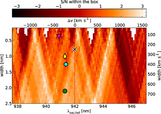
In Fig. 10, the 5σ noise determined as described in Section 3.4 is shown for the relevant central-wavelength/box-width space around the expected He II position and the S/N calculated over the same parameter space is shown in Fig. 11. While there might be indication of some excess at velocities between −450 and 0 km s−1, we do not find sufficient signal to claim a detection. The two masks giving the highest S/N 13 are a wider one with a width of 430 km s−1 at a central wavelength of 12 453 Å (z = 6.591, Δv = −160 km s−1) and a narrower one with a width of 100 km s−1 at a central wavelength of 12 447 Å (z = 6.588, Δv = −300 km s−1). The S/N in the two cases is after continuum subtraction 1.9 and 1.7, respectively. A somewhat higher S/N can be reached by using a narrower trace more centred on the position of the expected continuum.

5σ detection limits in a region around He II in extraction boxes of different widths and placed at different wavelengths corresponding to different velocity offsets w.r.t to the peak Ly α redshift of 6.595, which is marked by a red vertical line. For all boxes, the extent of the box in slit direction was 7 pixel. Further details are given in Section 3.4. The cross marks redshift and width of the Ly α line, while the yellow diamond and the green circle indicate our two fiducial boxes. Finally, the magenta triangle and the cyan hexagon indicate the two boxes giving the highest positive He II excess.
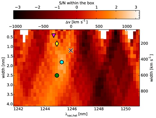
S/N ratio measured within extraction boxes equivalent to those included in Fig. 10. No continuum and telluric correction was applied for this plot. Maximum values are reached for boxes with λhel; vac = 12 453 Å with a velocity width of 430 km s−1 (cyan hexagon) and λhel; vac = 12 447 Å with a velocity width of 100 km s−1 (magenta triangle), respectively.
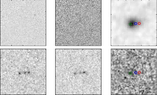
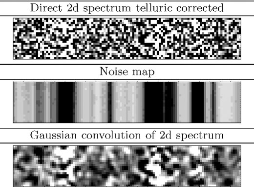
The 2D spectrum over the relevant velocity offset range is shown in Table 6 in the row labelled ‘observed’. The position of the default trace is indicated as magenta dashed lines in the smoothed figure, which is identical in the two columns, while the two extraction boxes giving the highest S/N are indicated by cyan vertical lines in the two columns, respectively. Additionally, a sky-spectrum over the same region and a Gaussian smoothed version are included. In the Gaussian smoothing, we excluded pixels being masked in our master high-noise pixel mask. For a guided eye, it might be possible to identify the excess visually. Yet, it is certainly possible that noise is seen and it cannot be considered a detection. It is noteworthy that there is a triplet of weak skylines in the centre of the region. While these skylines should in principle not increase the noise by much, as also being consistent with the error spectrum, this would assume an ideal sky subtraction. As can be seen in the figure, there are however some unavoidable residuals, extending over the complete slit.
2D spectrum and fake-source analysis for a wavelength range corresponding to the expected He II wavelength. In the row observed, the 2D spectrum in the region around the possible He II excess is shown. The grey-scale extends linearly between ±1 × 10⁻¹⁹ erg s−1 cm−2 Å−1 (white < black). Above a Gaussian smoothed version is shown with the same scale, at the top of which a sky-spectrum for the same region is included. Both the observed and smoothed images are identical in both columns. The magenta dashed horizontal lines indicate our default extraction mask. Below the observed row, images are shown, where Gaussian fake lines have been added with different strengths for two different FWHM and wavelength combinations. Widths and positions are indicated by the cyan vertical lines. The integrated flux in the respective fake lines is stated in the leftmost column.
 |
|
Note.aAdded line flux [10−18 erg s−1 cm−2].
2D spectrum and fake-source analysis for a wavelength range corresponding to the expected He II wavelength. In the row observed, the 2D spectrum in the region around the possible He II excess is shown. The grey-scale extends linearly between ±1 × 10⁻¹⁹ erg s−1 cm−2 Å−1 (white < black). Above a Gaussian smoothed version is shown with the same scale, at the top of which a sky-spectrum for the same region is included. Both the observed and smoothed images are identical in both columns. The magenta dashed horizontal lines indicate our default extraction mask. Below the observed row, images are shown, where Gaussian fake lines have been added with different strengths for two different FWHM and wavelength combinations. Widths and positions are indicated by the cyan vertical lines. The integrated flux in the respective fake lines is stated in the leftmost column.
|
|
Note.aAdded line flux [10−18 erg s−1 cm−2].
We tried to understand which line flux would be required for an excess to be considered visually a safe detections. We did this by adding Gaussians with FWHMs of 100 and 400 km s−1 centred on the wavelengths of the two extraction boxes leading to the highest S/N and assuming a spatial profile as expected for the continuum. The results are shown in Table 6. After visual inspection of four authors, we concluded that an additional flux of 2 × 10⁻¹⁸ and 4 × 10⁻¹⁸ erg s−1 cm−2 would be required in the two cases for a detection considered to be safe, corresponding as expected to approximately 5σ detections.
Finally, we estimated the 3σ upper limit on the He II EW0 in our fiducial 200 km s−1 extraction box, using the same continuum estimate as used for the continuum subtraction. This is a continuum flux density at the He II wavelength of 4.0 ± 0.5 × 10⁻²⁰ erg s−1 cm−2 Å−1, assuming the appropriate slit loss. This results in an upper limit of the observed frame EW of 75 ± 10 Å, which corresponds to a rest-frame EW0 of 9.8 ± 1.4 Å. The errors are due to the uncertainty in HF160W, not including the uncertainty in the continuum slope β.
3.6 High ionization metal lines
If Himiko's Ly α emission was powered either by a ‘type II’ or less likely by a ‘type I’ AGN, being disfavoured from the limited Ly α width, relatively strong C IV λ1549 emission would be expected. This would be accompanied by somewhat weaker N V λ1240, C III] λ1909, He II λ1640, and Si IV λ1400 emission lines (e.g. Vanden Berk et al. 2001; Hainline et al. 2011).
3.6.1 N V
N V λ1240 is a doublet consisting of two lines at 1238.8Å and 1242.8Å, respectively. With their oscillator strength ratio of 2.0: 1.0, the effective blend wavelength is 1240.2Å. The spectrum around N V is shown in the leftmost panel of Fig. 9. The hatched wavelength ranges mark the regions for the two N V lines under the assumption of our fiducial 200 km s−1 wide box. Weak and blended skylines, which are not marked by our skyline algorithm, and telluric corrected absorption causes the noise to vary strongly over the region.
Using the extraction aperture as shown in Fig. 9 and subtracting the continuum in the 2D frame as described in Section 3.4, we derive for the wider and narrower of our two fiducial boxes excesses of 0.7σ and 0.5σ, respectively, where we need to exclude a relatively high fraction of pixels due to high noise (cf. Table 5). The result is consistent with zero. Exploring the Δv–width parameter space for the S/N (Fig. 12), velocity offset and box-width can be chosen in a way to get a higher S/N. For example, boxes at +450 km s−1 with a width of 840 km s−1 per doublet component, corresponding to a single merged extraction box of 1324 km s−1, have an S/N of 3.4 with an included fraction of 42 per cent. However, such a relatively large offset towards the red from the Ly α redshift seems not feasible. Restricting the analysis to a more likely range of Δv from −500 to 0 km s−1, we would find a maximum S/N of 2.3 for box widths of 400 km s−1 at no velocity offset w.r.t to Ly α, with an included fraction in the box of 45 per cent. The flux within non-excluded pixels is 1.5 × 10⁻¹⁸ erg s−1 cm−2. A visual inspection of the relevant region does not allow for the identification of any line (Fig. 13).
Similar plot as shown for He II in Fig. 11. A telluric correction was applied to the underlying image and a continuum with a flux as motivated in Section 3.4 was subtracted. The S/N was calculated in two boxes at the respective wavelengths of the two individual lines (|$\lambda_\mathrm{rest}$|(N v):1238.82Å and 1242.80Å) w.r.t. to the blend centre.
Region around the N V λ1240 doublet, as expected based on the Ly α redshift. Upper: telluric corrected 2D spectrum, scaled between ± the minimum rms noise, σmin, in the shown region. Middle: noise map linearly scaled between σmin and 3σmin (white < black). The high noise regions are both due to skylines and due to regions requiring telluric correction. Lower: spectrum smoothed with a Gaussian kernel with a standard deviation of one pixel.
3.6.2 Other rest-frame UV emission lines
In Fig. 9, we are also showing cutouts for two further lines (C IV and C III]). The relevant wavelength range for the two components of C IV λλ1548, 1551, which have an oscillator strength ratio of 2.0:1.0, is located in a region of high atmospheric transmittance within the J band. While there are a few strong skylines, especially between the two components, there is enough nearly skyline-free region available. Visually, we do not see any indication for an excess. Also statistically, considering again the Δv range from −500 to 0 km s−1 w.r.t to the Ly α peak redshift, we find a maximum excess of 1.4σ after continuum subtraction.
By contrast, the C III] doublet is located between the J and H band, suffering from strong telluric absorption (cf. Fig. 9). Nevertheless, it could be possible to detect some signal in the gaps between absorption. Especially, the relevant part bluewards of the Ly α redshift has a relatively high transmission. Both the visual inspection and the formal analysis of the telluric and continuum corrected spectrum indicate no line. Detection limits for our fiducial boxes are stated in Table. 5.
Si IV λ1403 is also in a region of high atmospheric transmission. However, here the overall background noise in the spectrum is relatively high and as expected for this compared to C IV usually weak line, we do not see an excess.
Another line is N IV] λ1486, which has in rare cases been found relatively strong both in intermediate and high redshift galaxies (e.g. Christensen et al. 2012; Vanzella et al. 2010). Unfortunately, the spectrum is at the expected wavelength for N IV] covered with strong skylines (not shown).
The same holds for the [O III] λλ1661, 1666 doublet, which can be relatively strong in low-mass galaxies undergoing a vigorous burst of star formation (e.g. Erb et al. 2010; Christensen et al. 2012; Stark et al. 2014). We do not find any excess in the relevant wavelength range. As the region is in addition affected by several bad pixels, we do not state formal detection limits for this doublet.
4 DISCUSSION
4.1 SED fitting
We performed SED fitting including JF125W, HF160W, K, and IRAC 1–4, in total seven filters, where for IRAC3–4 only upper limits are available. As UKIDSS K and the IRAC data are not resolving the three components and a profile fit is with the available S/N not feasible, we fitted the three sources jointly by using the aperture corrected 2 arcsec diameter photometry (Table 4). Throughout our SED fitting we fixed the redshift to z = 6.590, a reasonable guess for the systemic redshift based on the Ly α line.
We used our own python-based SED fitting code coniecto, which allows both for an MCMC and a grid-based analysis. Here, we derived our results with the grid-based option. The code requires as input single age stellar populations (SSP) for a set of metallicities. Additionally, a pre-calculated nebular spectrum including continuum and line emission needs to be specified for each age–metallicity pair, and can be added to the respective SSP with a scalefactor between 0 and 1. This scalefactor can be understood as covering fraction, fcov, or |$1-f^\mathrm{esc}_\mathrm{ion}$|, with |$f^\mathrm{esc}_\mathrm{ion}$| being the escape fraction of the ionizing continuum. The inclusion of nebular emission has been found crucial for the fitting of redshift z ∼ 6–7 LAEs and LBGs (e.g. Schaerer & de Barros 2009, 2010; Ono et al. 2010).
SEDs for a given star formation history (SFH) are obtained by integrating the SSP. We were restricting our analysis to instantaneous bursts and continuous star formation. Due to the lack of deep enough rest-frame optical photometry in IRAC3–4, which would not be affected by strong emission lines at our object's redshift, it does not make sense to use more complicated SFHs. Already the used set of parameters allows for overfitting of the models.
We applied reddening to the integrated SEDs using the Calzetti et al. (2000) extinction law, assuming the same reddening both for the nebular and the stellar emission, motivated by evidence for the validity of this assumption in the high-redshift Universe (Erb et al. 2006).
As main input SSPs we used the models ‘Yggdrasil’ (Zackrisson et al. 2011), which include metallicities all from zero (Pop III) to solar (Z⊙ = 0.02). Their code consistently treats both nebular line and continuum emission (Zackrisson et al. 2001) by using Cloudy (Ferland et al. 1998) on top of stellar populations. We are here referring to SSPs as their publicly available instantaneous burst models. More details are summarized in Table 7.
| Parameter | Values |
|---|---|
| Yggdrasil | |
| Metallicities Z (Z⊙ = 0.02) | 0.0004, 0.004, 0.008 |
| 0.02, 0.0 (Pop III) | |
| IMFs | Kroupa (2001, 0.1–100 M⊙) |
| for Z = 0: Kroupa, | |
| lognormal (1–500M⊙, | |
| σ = 1 M⊙, Mc = 10 M⊙), | |
| Salpeter (50–500M⊙) | |
| Nebular emission | cloudy (Ferland et al. 1998) |
| Using: Schaerer (2002); Vázquez & Leitherer (2005); Raiter et al. (2010) | |
| BC03 (Padova 1994); nebular emission as in Ono et al. (2010) | |
| metallicities Z | 0.0001, 0.0004, 0.004, 0.008 |
| 0.02, 0.05 | |
| IMF | Salpeter (1955, 0.1–100 M⊙) |
| Nebular emission | following recipe described |
| in Ono et al. (2010) | |
| Using: Ferland (1980); Aller (1984); Storey & Hummer (1995); Krueger, | |
| Fritze-v Alvensleben & Loose (1995) | |
| Reddening | |
Notes. Calzetti et al. (2000) extinction law, assuming identical extinction for nebular emission and stellar continuum.
| Parameter | Values |
|---|---|
| Yggdrasil | |
| Metallicities Z (Z⊙ = 0.02) | 0.0004, 0.004, 0.008 |
| 0.02, 0.0 (Pop III) | |
| IMFs | Kroupa (2001, 0.1–100 M⊙) |
| for Z = 0: Kroupa, | |
| lognormal (1–500M⊙, | |
| σ = 1 M⊙, Mc = 10 M⊙), | |
| Salpeter (50–500M⊙) | |
| Nebular emission | cloudy (Ferland et al. 1998) |
| Using: Schaerer (2002); Vázquez & Leitherer (2005); Raiter et al. (2010) | |
| BC03 (Padova 1994); nebular emission as in Ono et al. (2010) | |
| metallicities Z | 0.0001, 0.0004, 0.004, 0.008 |
| 0.02, 0.05 | |
| IMF | Salpeter (1955, 0.1–100 M⊙) |
| Nebular emission | following recipe described |
| in Ono et al. (2010) | |
| Using: Ferland (1980); Aller (1984); Storey & Hummer (1995); Krueger, | |
| Fritze-v Alvensleben & Loose (1995) | |
| Reddening | |
Notes. Calzetti et al. (2000) extinction law, assuming identical extinction for nebular emission and stellar continuum.
For reasons of comparison to the SED fitting done by Ouchi et al. (2009, 2013), we also obtained results with input models as used in these works. These are based on BC03 (Bruzual & Charlot 2003) models, where a nebular emission is calculated by the prescription presented in Ono et al. (2010). We are referring in the following to these models as BC03–O10.
After calculating synthetic magnitudes on a large age–E(B − V)–Z–fcov grid, we have minimized χ2 w.r.t to mass for each parameter set. The grid covered ages between 0 and 800 Myr, with the upper limit being the age of the Universe at z = 6.59, and E(B−V) from 0.00 to 0.45. Used metallicities were those available in the input models (Table 7) and for fcov we allowed for three different values (0,0.5,1.0).
In Fig. 14, the results are shown for continuous star formation using the Yggdrasil models. For each point in the age–E(B−V) space the Z–fcov tuple allowing for the minimal χ2, |$\chi _{{\rm best}}^2$|, is chosen. The resulting |$\chi _\mathrm{best}^2$| contours are indicated in all five subplots, with the five subplots showing |$\chi _{{\rm best}}^2$|, stellar mass, star formation rate averaged over 100 Myr (SFR100)14, metallicity, and fcov, respectively. Stellar masses refer to the mass in stars at the point of observation.
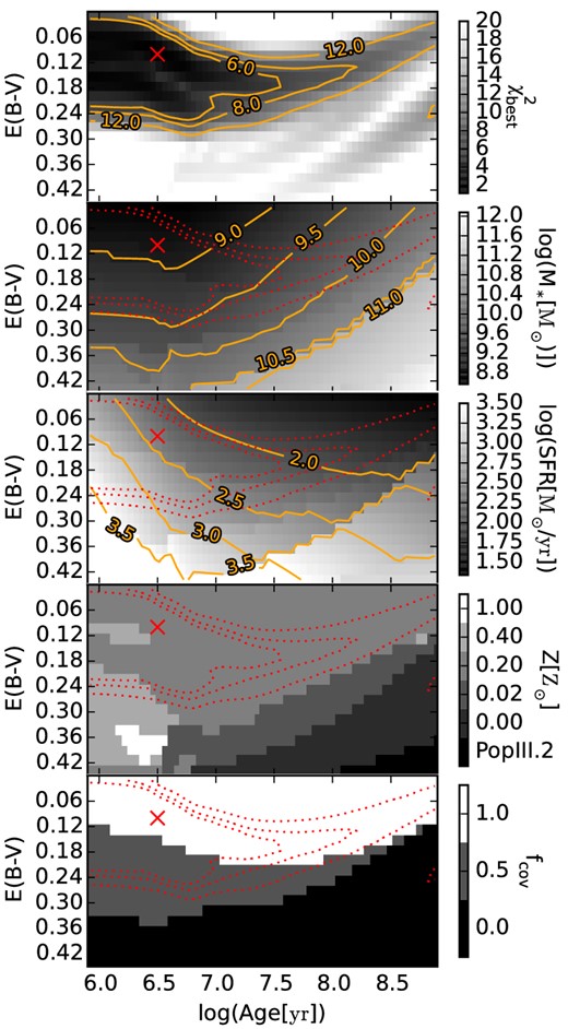
SED fitting results under the assumption of continuous SFH using the Yggdrasil models. Upper panel shows the lowest possible χ2 at a given point in the age–E(B−V) plain. Four physical quantities for the best models are shown below. For orientation, the same |$\chi _{{\rm best}}^2$| contours from the top plot are replicated as dotted line in each of the subplots. The model with the absolute minimal χ2 is marked as cross.
The global best-fitting SED over the explored parameter space is a very young |$3_{-2}^{+32}\,\mathrm{Myr}$| stellar population, which is strongly star-forming (SFR100 = |$2.3_{-1.2}^{+26.2}\times 10^2\,\,\mathrm{M}_{\odot }\,\mathrm{yr}^{-1}$|) and has a stellar mass of |$7_{-3}^{+32}\times \,10^8\,\mathrm{M}_{\odot }$| with a χ2 = 1.2.15 This best-fitting model is shown as cross in the maps and as SED in Fig. 15. The uncertainties on the estimated parameters were determined based on the range of models having χ2 < 6. A value of six can be understood as a good fit for seven filters.
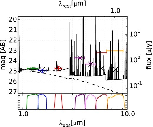
Best-fitting SED obtained with the Yggdrasil models under the assumption of continuous star formation. For this very young stellar-population (3 Myr) also the continuum is dominated by the nebular emission, showing the characteristics ‘jumps’ resulting from the bound-free recombination to different levels in hydrogen. The comparably weak stellar continuum is shown as dashed line. Synthetic magnitudes for the relevant filters are indicated as black crosses. The black circle is the magnitude measured from the spectral continuum.
Clearly, a large range of parameters is allowed. It is only for metallicity and reddening that relatively strong constraints can be inferred, with mainly Z = 0.2 Z⊙ models giving good fits and some Z = 0.4 Z⊙ models being allowed within χ2 < 6. Models with E(B − V) greater than 0.25 are unlikely. Further, at least partial nebular contribution is required. The wide range of solutions can be understood through the interplay of a somewhat evolved population with a 4000 Å break and strong nebular emission, combined with small amounts of dust extinction.
The strongest lines in IRAC1 and IRAC2 are [O III] λλ4959, 5007, and H α, respectively. The [O III] EW0 is expected to peak at metallicities around Z = 0.2Z⊙ (e.g. Finkelstein et al. 2013), strong enough to explain the blue IRAC1 − IRAC2 colour of −0.6 ± 0.2.
The |$\chi _{{\rm best}}^2$| plots are compared for burst and continuous star formation both using the Yggdrasil and the BC03–O10 model sets in Fig. 16. Burst models give acceptable fits only for very young ages, where they are basically identical to the continuous star formation models. Both model sets give consistent results, with small differences mainly existing where specific metallicities are only available in one of the two sets. For example, the area of relatively low |$\chi _{{\rm best}}^2$| at high ages for burst models using Yggdrasil is absent in the BC03–O10 models, as they require zero metallicity (Kroupa and lognormal IMF). However, these SEDs would require stellar masses in excess of 1011 M⊙ and can hence be considered infeasible. In general, biases are possible due to discretized metallicities.
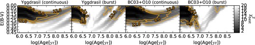
The left-hand panel shows the same as the upper panel in Fig. 14. For comparison, the |$\chi _{{\rm best}}^2$| result using the BC03+O10 models and the case of burst SFH is shown.
We also tested the impact of substituting our JF125W measurement with that of Ouchi et al. (2013). The fainter JF125W flux shifts the χ2 best contours slightly towards higher reddening and hence higher required SFRs, or alternatively higher ages. Ouchi et al. (2013) have found from their SED fitting with BCO3–O10 models under the assumption of continuous SFR a best-fitting model with a mass of |$1.5_{-0.2}^{+0.8}\times 10^{9}\,\mathrm{M}_{\odot }$|, an age of |$4.2^{+0.8}_{-0.2}\times 10^6\,\mathrm{yr}$|, and an |$E(B-V)=0.15^{+0.04}_{-0.03}$|, consistent with our results.16
If Himiko's extended Ly α emission was driven by merger activity between the three continuum bright objects, SFRs as high as a few 100 M⊙ yr−1 are expected, as seen e.g. in the simulations by Yajima et al. (2013) focusing on LABs, and consistent with our best-fitting model.
Importantly, a burst with the same properties as our best-fitting model having happened 100 Myr before the observed burst, would have faded in all detected filters by at least a factor 20. Hence, there could easily be a moderately young stellar population of a few 109 M⊙ without significantly contributing to the SED.
While this work was under revision, Schaerer et al. (2015) also published results from SED fitting for Himiko. Most importantly, they made use of the upper limit on the far-infrared luminosity, which can be estimated from the ALMA upper limit for the 1.2mm (observed-frame) continuum presented by Ouchi et al. (2013), in order to constrain the maximum allowed dust extinction.
Their obtained upper limit corresponds assuming a Calzetti et al. (2000) extinction law to E(B − V) < 0.05 ± 0.03, with the uncertainty due to the unknown dust temperature assumed for the conversion from continuum flux density to FIR luminosity. Using this upper limit, a huge part of the allowed parameter space can be ruled out. Schaerer et al. (2015) could argue, using for the SED fitting the photometry of Ouchi et al. (2013), that a young and heavily star-forming solution is disfavoured. However, due to the somewhat bluer F125W–F160W measured from the CANDELS data compared to that measured in the data of Ouchi et al. (2013), our fit requires somewhat less extinction and hence very young models consistent with their upper limit can be found.
4.2 Further SED considerations
As shown in Section 4.1, the observed broad-band magnitudes are compatible with models over a wide age, mass, and reddening range, where the single stellar population fit is likely an oversimplification of the problem. When looking at the JF125W –HF160W colour of the individual components (cf. Table 3), there exists a significant difference between the two more eastern and the westernmost component, with the latter being about 0.3 mag redder. This can all indicate differing stellar populations, differing escape fractions of the ionizing continuum, |$f^\mathrm{esc}_\mathrm{ion}$|, or differing amounts of dust.
Interestingly, the JF125W–HF160W ∼ −0.3 ± 0.1 of the two eastern components, corresponding to a β = −3.3 ± 0.6, is somewhat difficult to explain with a Pop II when taking account for nebular emission under the assumption of low ionizing continuum escape |$f^\mathrm{ion}_\mathrm{esc}$| (e.g. Bouwens et al. 2010). Only for complete escape of the ionizing radiation, a population with a metallicity as in our best-fitting SED (Z = 0.2 Z⊙) would produce a slope as steep as β = −3, whereas for |$f^\mathrm{ion}_\mathrm{esc}=0$| the steepest β is a about −2.5. By contrast, the best-fitting SED model requires a very low |$f^\mathrm{ion}_\mathrm{esc}$| to explain the IRAC magnitudes.
While each of the components does not differ more than 1.5σ from this β = −2.5, the fact that Ouchi et al. (2013) find at least for the two outer components similar results based on their independent data, increases the probability that the steep slope of Himiko–E is real. Certainly, possibilities exist to reconcile the blue colour of the individual components with the low escape fraction required by the SED model. For example there could be anisotropic ionizing escape in our direction, or the ionizing radiation could escape the star-forming regions and the nebular continuum emission is produced somewhat further out, making the nebular emission more extended than the stellar continuum.
Both the visual inspection of Fig. 4 and the spatial profiles in the individuals OBs (Fig. 5) indicate an offset of the overall continuum light w.r.t to the NB921 light distribution, which is dominated by the Ly α emission. The Ly α emission seems least strong around Himiko–W. This has been confirmed by the WFC3 / F098M imaging of Ouchi et al. (2013), who find the strongest Ly α emission originating from Himiko–E, which is with |${\rm EW}_{0} = 68^{+14}_{-13}$|, however not as high that it would put constraints on the escape fraction.
Two-photon, 2γ, continuum (Breit & Teller 1940), emitted by transitions between the 2s and 1s states of the hydrogen atom, is in the case of nebular emission powered by a central ionizing source one among other mechanism contributing to the continuum. In the case of cooling radiation, where the hydrogen atoms are collisionally excited, it would be the sole continuum contribution, though (Dijkstra 2009). Our data point provided by the spectrophotometry for the rest-frame wavelength range from 1238 to 1285Å could compared to F125W and F160W resemble the typical 2γ dip close to Ly α. Using the frequency-depended emissivities as stated in table 1 of Spitzer & Greenstein (1951), we calculate the expected JF125W − HF160W colour for the two photon continuum at z = 6.590. We find a value of JF125W − HF160W = −0.08. Therefore, it cannot be solely responsible for the found very blue JF125W − HF160W. In addition, we estimate for the peak flux density expected from cooling radiation based on the predictions of Dijkstra (2009) and the measured Ly α flux for Himiko a value of 28.3 mag. This is more than three magnitudes fainter than the measured flux. Therefore, 2γ emission from cooling radiation is unlikely to significantly contribute to the continuum.
Finally, we note that Ono et al. (2010) have favoured in their SED fitting for the composite of 91 NB921 selected LAEs at z = 6.6 a very young (∼1 Myr) and very low mass (∼108 M⊙) model, with significant nebular contribution (fescion = 0.2). They have only included those objects, which are not detected individually in IRAC 1,17 therefore excluding objects like Himiko. The IRAC 1 magnitude in their median stack is 26.6 mag. For Himiko, the total magnitude after the slightly uncertain aperture correction is 23.69 ± 0.09. Simplifying assuming that the flux in Himiko is equally distributed between the three sources, each of them would have a magnitude of 24.9. This is only a factor of 5 higher than the median stack. Therefore, the individual components are not as extremely different from the typical z = 6.6 LAEs as the joint photometry suggests.
4.3 Ly α profile
Due to resonant scattering the Ly α profile can be modified significantly both in the ISM/CGM and in the IGM. A shaping of the profile within the ISM/CGM is likely, with Ly α possibly entering the IGM with a typical double peaked profile observed for lower redshifts LAEs (e.g. Christensen et al. 2012; Krogager et al. 2013) as predicted by theory (e.g. Harrington 1973; Neufeld 1990; Verhamme, Schaerer & Maselli 2006; Laursen, Razoumov & Sommer-Larsen 2009). The blue or red peak is suppressed in the case of outflows or inflows, respectively.
On the other hand, Ly α could leave the CGM also with a nearly Gaussian profile, as seen in several cases for lower redshift LABs (e.g. Matsuda et al. 2006), and explainable theoretically by fluorescent Ly α emission in a fully ionized halo (e.g. Dijkstra, Haiman & Spaans 2006).
At z ≈ 6.5, the IGM is expected to always suppress the blue part of the Ly α line completely, while an extended damping wing might also suppress the red part to some extent, as for example found by Laursen et al. (2011), in accordance with previous observational (e.g. Songaila 2004) and analytical results (e.g. Dijkstra, Lidz & Wyithe 2007). Therefore, even when leaving the CGM as a Gaussian, the line might be reprocessed to the observed shape through scattering in the IGM. We tested the feasibility of this scenario for Himiko.
Assuming that the red slope of the profile is the nearly unprocessed Gaussian, we fit as a first test a line to this part only, similar to the approach used by Matsuda et al. (2006). We always added to the Gaussian a continuum as measured from the spectrum redwards of Ly α. The wavelength interval used for the fit is shown in Fig. 8 as horizontal bar and ranges from 9236.4 to 9250.0 Å.
The results from the formal fit are a redshift of |$6.589_{-0.013}^{+0.003}$|, a line FWHM of |$768_{-91}^{+317}\,\mathrm{km}\,\mathrm{s}^{-1}$| corrected for instrumental resolution, and a line flux of |$2.2_{-0.7}^{+8.1}\times 10^{-16}\,\mathrm{erg}\,\mathrm{s}^{-1}\,\mathrm{cm}^{-2}$| for this full Gaussian. The best-fitting flux value would correspond to a Ly α luminosity of 1.7 × 1044 erg s−1 after slit loss correction, and is a factor of 3.8 larger than the actually measured one.
The obtained FWHM is not unrealistically high. Matsuda et al. (2006) have found for LABs at z = 3.1 FWHMs of |$\gtrsim 500\,\mathrm{km}\,\mathrm{s}^{-1}$|. These high values were also confirmed by simulations (Yajima et al. 2013). For high redshift radio galaxies (HzRGs), the determined width would be still at the very lower limit (e.g. van Ojik et al. 1997).
Then, we tested whether the IGM absorption could indeed produce the observed Ly α profile of Himiko by fitting to a model where we apply the median IGM absorption curve of Laursen et al. (2011)18 to a Gaussian, assuming that the Gaussian's peak corresponds to the systemic redshift and convolving the result with the instrumental resolution (Fig. 8). For the fit of this combined model, we used a wavelength range including the full profile, ranging from 9220.3 to 9250.0 Å.
Under these assumptions the best-fitting underlying Gaussian has a redshift of |$6.59052_{-0.000\,04}^{+0.000\,06}$|, a line FWHM of |$702_{-13}^{+12}\,\mathrm{km}\,\mathrm{s}^{-1}$|, and a line flux of |$1.76_{-0.02}^{+0.02}\times 10^{-16}\,\mathrm{erg}\,\mathrm{s}^{-1}\,\mathrm{cm}^{-2}$|, where the uncertainties do not take account for the range of possible IGM absorption curves. The result, which is shown in Fig. 8 both before and after applying the median IGM absorption curve of Laursen et al. (2011), is surprisingly close to the observed profile save some small discrepancy at the peak. This demonstrates that IGM absorption alone is a valid option for shaping the Ly α profile of Himiko.
Summing it up, it is clear that from the observed Ly α shape alone little can be concluded about the full profile before entering the IGM. Therefore, the fraction of Ly α scattered out of the line of sight by the IGM is highly uncertain and upper limits on the flux ratios between rest-frame far-UV lines and those of Ly α, as required for the discussion in Section 4.4, need to be treated with caution.
The appropriate loss for Ly α can range from nearly zero, as would be the case for a single red peak produced by scattering of Ly α at an expanding optically thick sphere, to an enormous fraction in the case that we are only seeing a strongly suppressed red peak resulting from an infalling medium. Assuming the Gaussian as used for the model shown in Fig. 8 and comparing the flux to the actually measured one, about 38 per cent would pass the IGM.
As a compromise, we state in the following upper limits assuming 50 per cent flux loss in the IGM or alternatively, and more conservatively w.r.t to upper limits, zero flux loss to the IGM. In addition to the IGM absorption, the Ly α emission might also be reduced by dust, even so Himiko has been constrained to be very dust poor (Schaerer et al. 2015).
4.4 Implications from upper limits on rest-frame far-UV lines
As already outlined in the introduction, there is a range of possible mechanisms proposed to explain the extended emission around LABs. The most popular are photoionization either by a starburst, a (hidden) AGN, or radiative shocks caused by a burst of SN IIe following the onset of star formation. Alternatively, the powering mechanism could be gravitational cooling radiation. Possibly, a contribution from several mechanisms is jointly powering Himiko. While our upper limit measurements are not suited to identify minor contributions, we can compare them to the expectations for the different mechanisms assuming these as dominating.
For reference, measurements or upper limits on N V, C IV, He II, and C III] from the literature for a selection of composite spectra and interesting individual LABs and LAEs are listed in Table 8 and compared to the upper limits obtained by us for Himiko. The stated values are normalized by the respective Ly α fluxes.
Line ratios of He II, N V, C III], and C IV to Ly α as found in samples and individual objects by various studies. Upper limits are 3σ. References: [0]: line ratios as measured in this study for Himiko. The ratios are calculated based on slit loss corrected fluxes. While we have for Ly α assumed a spatial extent given by the narrow-band NB921 image, the other lines were corrected under the assumption that they are distributed as the continuum. If they were as extended as the resonant Ly α line, the upper limits would be a factor of 1.5 and 1.4 less stringent for N V and the three lines in the NIR arm, respectively. The non-detection limits are stated for our two fiducial boxes. Values in brackets are assuming a crude IGM correction of a factor of 2. [1]: SDSS quasar composite spectrum (Vanden Berk et al. 2001) [2]: composite spectra for AGNs among rest-frame UV-selected galaxies (Hainline et al. 2011). The sample is split into those with high and low Ly α EW0. To convert the values and the spread in the equivalent widths stated by Hainline et al. (2011) to values and spreads for the fluxes, we have used the continuum slopes of β = −0.1 ± 0.4 and β = −0.5 ± 0.3 stated by them for the composite spectra of the high and low EW0 sample, respectively. [3]: sample of nine HzRGs (Humphrey et al. 2008) [4]: Prescott, Dey & Jannuzi (2009) values are for their night 1. Ly α flux based on same aperture as other lines. [5]: Dey et al. (2005) Ly α flux is based on same aperture as other lines. [6]: Scarlata et al. (2009) referring to component Ly1; Ly α flux based on same aperture as other lines. [7]: 1σ He II detection from HST/WFC F130N NB imaging (Cai et al. 2011) [8]: He II non-detection for extreme Ly α EW0 ≈ 900Å object (Kashikawa et al. 2012) [9]: He II non-detection for SDF J132440.6+273607 (Nagao et al. 2005) [10]: 109 M⊙ LAE at z = 2.3, showing strong He II and C III] emission likely powered by star formation (Erb et al. 2010).
| Ly α | N V | C IV | He II | C III] | |
|---|---|---|---|---|---|
| Himiko | |||||
| Based on aperture corrected line fluxes and upper limits without (with) IGM correction | |||||
| box: 200 km s−1; voff = −250 km s−1 | 1.00 | <0.04 (<0.02) | <0.15 (<0.07) | <0.07 (<0.03) | <0.12 (<0.06) |
| box: 600 km s−1; voff = −250 km s−1 | 1.00 | <0.08 (<0.04) | <0.25 (<0.13) | <0.10 (<0.05) | <0.18 (<0.09) |
| Composite spectra | |||||
| Broad-line AGN [1] | 1.00 | 0.03 | 0.25 | 0.005 | 0.16 |
| Narrow-line AGN [2] | 1.00 | 0.05 ± 0.01 | 0.20 ± 0.04 | 0.07 ± 0.02 | 0.16 ± 0.07 |
| EWLy α > 63 Å | |||||
| Narrow-line AGN [2] | 1.00 | 0.16 ± 0.05 | 0.25 ± 0.09 | 0.17 ± 0.06 | 0.17 ± 0.09 |
| EWLy α < 63 Å | |||||
| Radio-galaxies (z ∼ 2.5) [3] | 1.00 | 0.04 | 0.15 | 0.09 | 0.06 |
| Example LABs | |||||
| LAB PRG1 (z = 1.67) [4] | 1.00 | <0.39 | <0.09 | 0.12 | <0.07 |
| LAB (z = 2.7) [5] | 1.00 | <0.02 | 0.13 | 0.13 | 0.02 |
| LAB (z = 2.38) [6] | 1.00 | N/A | <0.45 | 0.36 | N/A |
| Example LAEs | |||||
| LAE IOK (z = 6.96) [7] | 1.00 | N/A | N/A | 0.06 ± 0.05 | N/A |
| LAE SDF-LEW-1 (z = 6.5) [8] | 1.00 | N/A | <0.013 | <0.015 | N/A |
| LAE SDF (z = 6.33) [9] | 1.00 | N/A | <0.675 | <0.340 | N/A |
| BX418 [10] | 1.00 | N/A | abs | 0.034 | 0.048 |
As Ly α and the other lines might have different spatial extent, we calculated the ratio between these lines and Ly α for Himiko in two different ways. In both cases, we converted before taking the ratio both Ly α and the upper limits to aperture corrected values, but while assuming in the first case that potential emission is as extended as Ly α, we assumed in the second case that the emission from other lines is co-aligned with the continuum. The values for the first case are identical to those one would obtain from taking the ratios with Ly α measured in the same apertures19 as used for the determination of the line flux upper limits.
4.4.1 Stellar population
The range of SED models which give reasonable good fits allows for SFR100 ranging from about 100 M⊙ yr−1 to extreme 2600 M⊙ yr−1. The Ly α fluxes and rest-frame equivalent widths for these models are between 6 × 10⁻¹⁷ and 37 × 10−17 erg s−1 cm−2 and between 72 and 296 Å. These values were extracted from the Yggdrasil SEDs by using the same approach as for the observation, meaning a continuum measurement at a rest-frame wavelength of 1262 Å. Further, the same extinction law as for the rest of the galaxy was assumed for Ly α. These values mean that Himiko's observed Ly α flux and EW0 can easily be accounted for by the strong Pop II star formation. Even a relatively strong IGM correction or destruction of Ly α by dust in the ISM would not pose a problem.
Still, an interesting question is whether in this heavily star-forming galaxy Pop III star formation might be ongoing 800 Myr after the big bang or whether our upper limit for He II allows us to rule it out. The comparison of a measured He II EW0 to theoretical models can put very strong constraints on the allowed IMF–metallicity–age parameter space. Combining the information about He II with an intrinsic Ly α EW0 would allow us to tighten the constraints even further. However, Ly α's susceptibility to resonance effects weakens its usefulness for this purpose. He II is not affected by this problem. As we do not detect He II, we can only test whether we would expect for Pop III star formation He II flux above our non-detection limit.20
Using the EW0 predictions for He II and Ly α calculated by Raiter et al. (2010), and following the approach by Kashikawa et al. (2012) for the LAE SDF-LEW-1, we applied this tool to Himiko. In Fig. 17, the predictions are shown for two different IMFs and six different metallicities ranging from zero to solar, and assuming constant star formation. In addition, both for zero metallicity and Z = 0.004 = 0.2 Z⊙ values are included for burst models. Both IMFs, Salpeter, and B, are power-law IMFs with Salpeter (1955) slope of α = 2.35, however differing in the mass-range with 1–100M⊙ and 1–500M⊙, respectively.
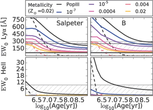
Shown are both the Ly α and the He II|$\mathrm{{\rm EW}}_0$| for two different IMFs assuming constant star formation, where B has also a Salpeter slope, but includes stars up to 500 M⊙. We are showing the values for six different metallicities, ranging from Pop III (Z = 0) to solar metallicity (Z = 0.02). In addition, burst models are included for Pop III and Z = 0.004 as dashed lines. Models have larger EW0 with decreasing metallicity. The measured Ly α EW0 is the thick lower horizontal line, while the 3σ upper limit on He II is shown as a shaded area. More details are given in Section 4.4.1
In the figure, both the directly observed Ly α EW0 and the one obtained for the Gaussian fit to the red wing (Section 4.3) are shown as horizontal lines. The range of allowed EW0's from the SED fitting is indicated as shaded area. For He II, the 3σ upper limit for our fiducial 200 km s−1 box is represented as shaded area.
Assuming that the intrinsic Ly α EW0 is the directly measured one, even a solar metallicity (Z⊙ = 0.02) population with standard Salpeter IMF and continuous star formation would be independent of the age above the observed EW0. The approximate correctness of the red wing fit would allow for significantly stronger constraints. Then, basically only Pop III and very metal-poor models up to Z = 10−5 would be allowed for continuous ages larger than about 10 Myr. Populations with higher metallicity would need to be younger. As indicated by our SED fitting, young ages are certainly possible, and very low metallicities are even in the case of strong IGM absorption not necessarily required.
For a Salpeter IMF with 1–100M⊙, only an extremely young (<1 Myr) metal-free population could produce an He II EW0 above the 3σ detection limit of 9.8 Å, independent of IMF, while for the high-mass IMF B He II flux would be detectable over a longer period at least for a Pop III. Here, it is important to note that detectable He II would be accompanied by very high Ly α EW0. Summing it up, it is only a very young Pop III with an IMF producing very heavy stars, which can be ruled out based on the He II upper limit.
C III], [O III] λλ1661, 1666, and at least in some cases also C IV emission, created by photoionization in the H II regions surrounding young high-mass stars, is now understood to be relatively common in low-mass galaxies with high specific star formation rates and low metallicities (e.g. Fosbury et al. 2003; Erb et al. 2010; Christensen et al. 2012; Stark et al. 2014). While not as strong as in AGNs, the typically strongest of these lines is C III], which has been found with EW0 up to ∼15 Å (Stark et al. 2014).21 A detection of this line seems to be correlated with high Ly α EW, with the correlation probably being a result of both line strengths depending on metallicity (Stark et al. 2014).
Our 3σ upper limit for C III] EW0 is due to the lines’ location between J and H band with EW0 < 23Å for the 200 km s−1 extraction box larger than the observed values. Only if the lines were close to unresolved and the velocity offset with respect to peak Ly α would allow for relatively high transmittance (cf. Fig. 9), a detection would have been feasible. Similar, one or both of the [O III] λλ1661, 1666 lines, which can be almost as strong as C III], would be only for very specific velocity offsets w.r.t to Ly α within the skylines gaps. Therefore, little can be concluded from these non-detections about the presence of a substantial population of young massive stars, which in principle could help to break the degeneracy in the SED fitting.
4.4.2 Illumination by (hidden) AGN
Quasars are well known to be responsible for strong Ly α emission in so-called extended emission line regions (EELRs) spreading in some cases over several 100 kpc. When being switched on during the phase of cold gas accretion, Haiman & Rees (2001) predicted this emission to originate from the illumination of primordial gas. However, at least at lower redshifts, the illuminated gas is more likely ejected galaxy material driven out by either SNe or the jets of the AGN itself (e.g. Villar-Martín 2007), resulting in the illumination of metal enriched gas and hence a multitude of emission lines.
With Himiko's three spatially distinct components all located within about 6 kpc transverse distance and no strong evidence for much difference in the line of sight direction, they are likely in the process of merging and hence triggered AGN activity is not unlikely. Further, Ly α emission powered by AGNs is a common and expected phenomenon. When considering AGNs, it can be useful both to subdivide between radio-quiet and radio-loud (e.g. McCarthy 1993), and between obscured (‘type II’) and non-obscured (‘type I’) by a dusty torus. Extended emission has been found for all cases (e.g. Matsuoka 2012). In the following, we are discussing all four options for Himiko, especially w.r.t to our non-detection limits.
As discussed by Ouchi et al. (2009), neither of the existing X-ray (XMM–Newton), 24 μm (Spitzer MIPS), and sub-mm (850 μm SCUBA) data are deep enough to rule out a type I quasar, when scaling the Elvis et al. (1994) quasar template to the rest-frame VIS IRAC 1 flux. However, there is a strong argument against a type I AGN in the Ly α width, which is even after accounting for IGM absorption too narrow to be originating from a type I AGN (cf. Section 4.3). Another argument against a quasar, at least for the two eastern components, is the continuum slope. Davis, Woo & Blaes (2007) find for SDSS quasars a mean slope of β = −1.6322 and very few objects with slopes bluer than β = −2.0 for the wavelength range between 1450Å and 2200Å. Although the redshifts of this sample is limited to 1.67 ≤ z ≤ 2.09, we do not expected the quasar spectra to be much bluer for higher redshifts. Therefore, it is unlikely that the two eastern components are dominated by direct continuum emission from the accretion disc. Finally, our 3σ upper limit on C IV/Ly α of 0.13, using the 600 km s−1 aperture and assuming a crude IGM correction of a factor of 2 is two times below the typical value for type I quasars in the composite spectrum of Vanden Berk et al. (2001). Certainly, this comparison falls somewhat short, as a C IV width of 600 km s−1 is too low for a type I quasar. Much higher widths are not justifiable based on our observed Ly α line width.
By contrast, Himiko's Ly α width is an option for the extended emission line regions around quasars, may it be either a powerful HzRG or a radio quiet type II quasar. While typical Ly α line widths of ∼1000 km s−1 seem somewhat high compared to Himiko's measured one, it might be possible to explain such a width under the assumption of strong IGM absorption (cf. Section 4.3). Further, it is known that HzRGs with very relaxed kinematics exist. MRC 0140–257 has over the complete nebula Ly α |${\rm FWHM} \lesssim 500\,\mathrm{km}\,\mathrm{s}^{-1}$| (Villar-Martín et al. 2007), with very narrow emission in the peaks of Ly α surface brightness (FWHM ∼ 250 km s−1). Also, while the extended Ly α emission around HzRGs is usually spatially kinematically disturbed by several 100 km s−1, MRC 0140–257 has comparable low velocity offsets. Himiko would need to be similar to this rather special object, as we see in our stacked spectrum no evidence for strong velocity gradients (cf. both Figs 6 and 7). We remark that velocity gradients could be smoothed out in our stack, as it is a superposition of observations with different slit angles. However, also in the spectrum of Ouchi et al. (2009), who observed with a fixed slit position, only a small Ly α velocity gradient of 60 km s−1 is found over the east–west direction.
Comparing the rest-frame UV and optical photometry, we find that the magnitudes measured for Himiko are indeed values reasonable for those expected from HzRGs, when taking the strong and extended emission in the EELRs into account. Assuming a flat continuum in fν and HF125W (24.93 mag) as normalization, we can estimate the flux due to emission lines in IRAC1 and IRAC2 to 14.8 × 10⁻¹⁷ erg s−1 cm2 and 4.8 × 10⁻¹⁷ erg s−1 cm−2, respectively, corresponding to a ratio of 3.1. Summing up the relevant line fluxes in the HzRG composite spectrum of Humphrey et al. (2008), a typical emission line flux ratio of 3.0 between IRAC1 and IRAC2 would be obtained,23 consistent with that measured for Himiko. Assuming that about 70 per cent of the line flux in IRAC1 is due to [O III] λ5007, the [O III] λ5007 rest-frame EW0 would be 1400 Å. Such a value is not unrealistic for HzRGs (e.g. Iwamuro et al. 2003). Finally, based on the [O iii] flux estimated above, Himiko's Ly α flux would be using the Humphrey et al. (2008) average ratio expected to be a factor of 1.7 higher than the actually observed one. This factor is easily within the uncertainty of the IGM absorption correction.
While this similarity in line ratios is interesting, it is not entirely surprising when considering our best-fitting stellar SED model. Humphrey et al. (2008) conclude, that the line emission in these HzRGs is not mainly powered by the interaction of the radio lobes with the gas, but rather by photoionization, and that the illuminated gas has typical metallicities of Z = 0.2 Z⊙.
A means to discern between an AGN or a young stellar population as ionizing source would be through the strength and ratios of rest-frame far-UV emission lines. The ratios between these lines and Ly α are in general expected to be stronger, when being powered by an AGN.
A complicating factor when interpreting non-detection limits is the extent of the possible line emission. Extended Ly α emission could be a consequence of resonant scattering or of in situ production by ionizing radiation escaping the ISM. In the first case other emission lines would be almost co-aligned with the UV continuum, while in the latter case they could be spatially extended as the Ly α emission (e.g. Prescott et al. 2015), resulting for our object in a larger slit loss.
The typical ratio between C IV and Ly α in the Humphrey et al. (2008) composite is with 0.15 similar to the 3σ upper limit for our target, when assuming the 600 km s−1 extraction box and a crude Ly α IGM correction of a factor of 2, which corresponds to C IV/Ly α <0.13 and <0.18 assuming a spatial extent similar to the continuum or the Ly α emission, respectively. Also, the typical He II/Ly α of 0.09 would be detected with at least 3σ even for He II emission as extended as Ly α, assuming again the crude IGM correction and the wider extraction box. The advantage of He II compared to C IV is that it would be present even when assuming primordial composition of the illuminated gas.
Another problem with the interpretation of Himiko as an HzRG is the available 100 μJy 1.4 GHz VLA upper limit (Simpson et al. 2006). Assuming example radio spectral indices of −0.5, −1.0, and −1.5, with ultrasteep slopes more typical for high-z galaxies, this corresponds to L1.4 GHz of 1.8 × 1025, 5.0 × 1025, 1.4 × 1026 W Hz−1. Converted to 5 GHz the upper limit would be around 1–2× 1025 W Hz−1 and hence at the very lower limit of what would still be considered a radio-loud galaxy according to the classification by Miller, Peacock & Mead (1990). On the other hand, if the main ionizing source for the EELRs is photoionization by the quasar and not the radio jets, the non-detection in the radio data is not ruling out the possibility of a hidden AGN as powering source. Indeed, EELRs have been found around the less known population of radio-quiet type II quasars (e.g. Gandhi, Fabian & Crawford 2006; Villar-Martín et al. 2010).
For several among the z ≈ 2–3 LABs, a hidden AGN has been identified at least as a partial contributor to the Ly α ionizing flux. For example the blob of Dey et al. (2005) at z ≈ 2.7 shows clear indication of a dust-enshrouded AGN, producing both He II and C IV emission with relatively narrow width (∼365 km s−1). Scaling the strength of the lines to our Ly α surface brightness, both lines should be detected.
For the narrow-lined AGNs among those UV-selected galaxies by Steidel et al. (2004) at z ∼ 2–3 (Hainline et al. 2011), the ratios between the rest-frame far-UV lines and Ly α would be even higher.
In addition to the constraints presented here, Baek & Ferrara (2013) have argued for a criterion to discriminate between LABs being powered by either star formation, Compton-thin, or Compton-thick AGNs based on the combined information about the observed surface brightness profile and skewness of the Ly α line. They seem to conclude that Himiko is not in the right region of the parameter space for having an AGN as source.
4.4.3 Gravitational cooling radiation
Early semi-analytical models assumed that the gas feeding a halo is heated to the virial temperature. However, cosmological SPH simulations indicate that the majority of the infalling gas might never reach these high temperatures (Fardal et al. 2001). Under the assumption of primordial element composition, meaning basically only H and He, the major cooling channel of the gas is consequently not through Bremsstrahlung, as for gas with temperatures above 106K, but through collisional excitation of hydrogen and, depending on the temperature, also through He II. Collisional excitation cooling peaks at 104.3K and 105K for H I and He II, respectively.
For several observed LABs in the literature, it has been suspected that cooling radiation is the major driver of the extended Ly α emission. For instance, Nilsson et al. (2006) had favoured this scenario for their LAB at z = 3.16, as they could not identify an obvious counterpart, even in deep the Great Observatories Origins Deep Survey (GOODS) HST imaging. Recent reanalysis of this object based on the extended availability of multiwavelength data allowed Prescott et al. (2015) to identify one of the objects in the field, which is located at a distance of about 30 kpc from peak Ly α emission, as an obscured AGN. Unfortunately, no spectrum deep enough to seriously probe He II and the other rest-frame far-UV lines is available for this object.
A LAB, where He II has been observed, is the one by Scarlata et al. (2009). While an AGN can also be identified photometrically within this object, they favour gravitational cooling radiation being at least partially responsible for He II because of the non-detection of C IV.
The He II luminosity of 8 × 1041 erg s−1 within their extraction mask would correspond at z = 6.595 to a flux of 1.6 × 10⁻¹⁸ erg s−1 cm−2, a flux which would not be safely detectable by us. On the other hand, scaling He II to the higher Ly α flux in Himiko, we would be able to significantly detect it (cf. Table 8).
The question is whether the corresponding high He II luminosity would be at all feasible for cooling radiation and whether a substantial amount of the Ly α emission could originate from cooling radiation. Insight can be gained by comparison to published results from simulations.
As a relatively narrow-line is predicted for He II in the case of cooling radiation (Yang et al. 2006), we compare to the 3σ upper limit of our standard 200 km s−1 aperture. This limit corresponds to a luminosity of |$L_{\mathrm{{He}\,{\small {II}}}}=1.5\times 10^{42}\,\mathrm{erg}\,\mathrm{s}^ {-1}$|, a value high compared to the luminosities of even the heaviest haloes in the simulations of Yang et al. (2006). Here, it needs to be noted that the results of Yang et al. (2006) are for z = 2.3.
Yajima et al. (2015) have run a hydrodynamical simulation combined with Ly α radiative transfer, including all radiative cooling and heating, star formation in a multiphase ISM, stellar feedback, and UV background. Their simulation traces a halo developing a Milky Way size galaxy over cosmic times. We have extracted from their presented evolution plots several quantities at redshift z = 6.6. A fraction of 65 per cent of Ly α is predicted by them to be due to cooling radiation, mainly created within the cold accretion streams, where the total Ly α luminosity is LLy α = 4.5 × 1042erg s−1. Therefore, even before correcting for IGM absorption and before applying a surface brightness threshold, the Ly α luminosity is more than a factor of 10 lower than Himiko's Ly α luminosity.
Taken this and the fact that the SED fitting suggest vigorous star formation, it is unlikely that a major fraction of Himiko's Ly α luminosity is produced by cooling radiation. Therefore, as each particle in the simulations of Yang et al. (2006) has |$f_{{\rm He}\,\small {II}\lambda 1640} \le 0.1\times f_{\mathrm{Ly}\,\alpha }$|, the He II flux is not very likely to be detectable and no strong conclusions can be drawn from the non-detection.
4.4.4 Shock ionization
Another possible explanation for strong and extended Ly α emission are large-scale shock-super-bubbles (Taniguchi & Shioya 2000), which might be the consequence of galactic winds powered by a large number of core-collapse SNe within the first few 100 Myr after the onset of the initial starburst (Mori, Umemura & Ferrara 2004; Mori & Umemura 2007). Assuming that the kinetic energy of the SN ejecta is converted into radiation by fast-shocks and combining information on C IV/He II and N V/He II ratios with a measured line width, one could get insight into the feasibility of this mechanism as contributing power source for the extended Ly α emission through comparison to shock model grids (e.g. Allen et al. 2008). In absence of a significant detection of at least one of the lines, such an analysis is not feasible.
5 CONCLUSION
With our analysis, we add further hints to the puzzle of what is powering the remarkable Ly α emitter Himiko.
First, we have detected a continuum in the spectrum showing a clear break at the wavelength of Ly α, ruling out any remaining chance of it being a lower redshift interloper. The fact that the continuum appears like a single step function indicates that there are no large velocity differences between the three distinct UV bright components.
From SED fitting, including CANDELS JF125W and HF160W data, we argue for a young and heavily star-forming stellar population, with a total stellar mass of the order of 109 M⊙ and a metallicity of Z = 0.2 Z⊙, with the bright IRAC1 magnitude explained by very strong [O III] emission. While we find that similar broad-band magnitudes would also be produced by lines in the extended emission line regions around HzRGs, this scenario is for several reasons more unlikely. Among them is the most important result of this work. Our upper limits on important rest-frame far-UV lines are clearly disfavouring an AGN as sole powering source for the extended Ly α emission. However, due to the natural lack of knowledge about the appropriate slit loss, line-width, and systemic redshift and the spread in line strength for AGNs, it is not entirely impossible that an AGN has escaped our detection.
Based on observations made with ESO telescopes at the La Silla Paranal Observatory under programme ID 087.A-0178(A). The Dark Cosmology Centre is funded by the DNRF. JPUF and PL acknowledge support from the ERC-StG grant EGGS-278202. This work is based on observations taken by the CANDELS Multi-Cycle Treasury Program with the NASA/ESA HST, which is operated by the Association of Universities for Research in Astronomy, Inc, under NASA contract NAS5-26555. This research made use of astropy, a community-developed core python package for Astronomy (Astropy Collaboration, 2013). We thank Martin Sparre for providing us with his python XSHOOTER pipeline manager, and Nobunari Kashikawa and Yoshiaki Ono for providing us with information.
NOTE ADDED IN PROOF
Very recently Matthee et al. (2015) have discovered based on a ∼ 5 deg2 NB survey that very bright LAEs at z = 6.6, similar to Himiko, might not be as rare as previously assumed. Further, Sobral et al. (2015) have presented for the two most extreme objects in the COSMOS part of this sample spectroscopic follow-up and found for the brightest object in addition to Ly α also strong He II λ1640 emission, possibly indicative of a Pop III.
Currently, the spectroscopically confirmed LAE with the highest redshift (z = 7.5; Finkelstein et al. 2013) has been found with HST/WFC3 broad-band data.
We used the FITS header keyword HIERARCH ESO TEL IA FWHM. We tested the use of this keyword with a number of standard and telluric stars. We found that the FWHM values based on this keyword on average agree with a scatter of about 0.2 arcsec with the Gaussian FWHM measured from the spatial profile.
xsh_scired_slit_nod
As ESO does not take by default enough dark frames for such deep observations, we needed to use frames from several days around the observations for this test. In the nodding reduction used for our result no dark frames are required.
Based on comparing different flat-fields, we concluded that the throughput of the K-blocking filter in the 0.9 arcsec × 11 arcsec JH slit is in the J band ≳ 97 per cent.
We have used the reference spectra from pipeline version 1.5.0, as those from pipeline 2.3.0 do not allow for cross-calibrations of the same quality.
http://www.nottingham.ac.uk/astronomy/UDS/data/dr8.html. We obtained the data from the WFCAM science archive (Hambly et al. 2008).
SExtractor keywords (FLUX_APER / MAG_APER).
We created fake images with the iraf task mkobjects.
RA, DEC = |$2^{\rm h}17^{\rm m}57 {.\!\!\!\!^{{\mathrm{s}}}}563$|, −05°08′44|${^{\prime\prime}_{.}}$|45 for the centroid of the Ly α emission.
Ly α: λrest = 1215.7 Å.
As the JF125W magnitude of Ouchi et al. (2013) is fainter, this results in higher upper limits both for the line fluxes and the EW0.
Formally, a very narrow box close to the strong skylines at ∼+ 1000 km s−1 gives a similar high S/N. However, this is clearly affected by residuals from strong skylines.
If the age of the stellar population is smaller than 100 Myr, it is averaged over the population age. SFR100 is identical to the instantaneous SFR for a constant SFH.
Not reduced χ2.
In the original publication a different best-fitting model was stated 1.5 × 10¹⁰ M⊙, an age of 1.8 × 10⁸ yr, E(B − V) = 0.15, and an SFR of 100 M⊙ yr−1; erratum in preparation.
Based on Spitzer/SpUDS (Dunlop et al. 2007), which is less deep than Spitzer/SEDS.
Reionization starting at z = 10.
Meaning same slit-width and extraction aperture height.
We are referring here as Pop III to a zero metallicity population.
In the spectrum of the Lynx arc (Fosbury et al. 2003) higher EWs have been measured for these rest-frame UV lines. However, these extreme EWs are not in agreement with self-consistent photoionization models and might be a result of differential gravitational lensing between illuminated gas and illuminating stars (e.g. Villar-Martín, Cerviño & González Delgado 2004).
Converted from the να as stated in Davis et al. (2007) to λβ.
The relevant lines in IRAC1 are He II λ4686, H β, and [O III] λλ4959, 5007 and in IRAC2 O I λ6300, H α, and [N II] λλ6548, 6583.
