


Abstract
We present weak lensing and X-ray analysis of 12 low-mass clusters from the Canada–France–Hawaii Telescope Lensing Survey and XMM-CFHTLS surveys. We combine these systems with high-mass systems from Canadian Cluster Comparison Project and low-mass systems from Cosmic Evolution Survey to obtain a sample of 70 systems, spanning over two orders of magnitude in mass. We measure core-excised LX–TX, M–LX and M–TX scaling relations and include corrections for observational biases. By providing fully bias-corrected relations, we give the current limitations for LX and TX as cluster mass proxies. We demonstrate that TX benefits from a significantly lower intrinsic scatter at fixed mass than LX. By studying the residuals of the bias-corrected relations, we show for the first time using weak lensing masses that galaxy groups seem more luminous and warmer for their mass than clusters. This implies a steepening of the M–LX and M–TX relations at low masses. We verify the inferred steepening using a different high-mass sample from the literature and show that variance between samples is the dominant effect leading to discrepant scaling relations. We divide our sample into subsamples of merging and relaxed systems, and find that mergers may have enhanced scatter in lensing measurements, most likely due to stronger triaxiality and more substructure. For the LX–TX relation, which is unaffected by lensing measurements, we find the opposite trend in scatter. We also explore the effects of X-ray cross-calibration and find that Chandra calibration leads to flatter LX–TX and M–TX relations than XMM–Newton.
1 INTRODUCTION
Precise knowledge of the total mass of galaxy clusters is a crucial ingredient in order to probe cosmology by means of cluster number counts. Cluster masses can be inferred by means of gravitational lensing, from the velocity dispersion of cluster galaxies assuming dynamical equilibrium, or from X-ray surface brightness and temperatures assuming hydrostatic equilibrium (HSE). However, these direct methods are observationally expensive, especially for low-mass systems and at high redshifts. Fortunately, cluster mass scales with observational properties such as X-ray luminosity and temperature. Therefore it is possible to calibrate robust and well-understood scaling relations between cluster mass and observables, in order to be able to study statistical samples of clusters as cosmological probes.
Both simulations and observations show that clusters are found in various dynamical states, with bulk motions and non-thermal pressure components present in the intracluster gas. These affect mass measurements relying on dynamical equilibrium or HSE. In particular, as indicated in both simulations (e.g. Nagai, Kravtsov & Vikhlinin 2007; Shaw et al. 2010; Rasia et al. 2012), observations (e.g. Mahdavi et al. 2008, 2013; Kettula et al. 2013b; Donahue et al. 2014; Israel et al. 2014, 2015; von der Linden et al. 2014b) and recent analytical work by Shi & Komatsu (2014), HSE mass estimates differ from the lensing mass. The trend in the above studies is that HSE mass estimates underestimate the true mass by ∼10–30 per cent. However, as shown by e.g. the recent systematic comparison of mass estimates by Sereno & Ettori (2014), there is significant disagreement between different mass estimates relying on the same method. Though cluster triaxiality and substructure may complicate the interpretation, gravitational lensing provides the most reliable way of determining the true cluster mass, as it requires no assumptions on the thermodynamics of the intracluster gas or the dynamical state of the cluster.
In the self-similar case which assumes pure gravitational heating, cluster observables and mass are related by power-laws (Kaiser 1986). However, the relative strength of baryonic physics increases at low masses. Analysis by e.g. Nagai et al. (2007), Giodini et al. (2010), McCarthy et al. (2010), Stanek et al. (2010), Fabjan et al. (2011), Le Brun et al. (2014), Planelles et al. (2014) and Pike et al. (2014) indicate that baryonic processes such as non-gravitational feedback from star formation and active galactic nuclei (AGN) activity are expected to bias scaling relations from the self-similar prediction. The above works also indicate that the deviations are expected to be stronger for groups and low-mass clusters than for high-mass clusters. Hydrodynamical simulations by Schaye et al. (2010) show that the gas removed by AGN activity in groups can also affect the large-scale structure out to several Mpc, potentially skewing cosmic shear measurements (Semboloni et al. 2011; van Daalen et al. 2011; Semboloni, Hoekstra & Schaye 2013; Kitching et al. 2014). Consequently, characterization of the effects of feedback at group and low-mass cluster level is of high interest for both cluster and cosmic shear studies.
Indeed, recent detailed observations of groups and low-mass clusters by e.g. Sun et al. (2009), Eckmiller, Hudson & Reiprich (2011) and Lovisari, Reiprich & Schellenberger (2015) have reported evidence pointing to the direction of such mass-dependent deviations from self-similar scaling (see also Giodini et al. 2013, and references therein). Even if a direct measurement of a break in the scaling relations is hard, relations fitted to groups tend have a larger intrinsic scatter than similar relations fitted to massive clusters. However, most previous studies rely on X-ray mass estimates based on HSE. The HSE condition is broken by the same feedback processes affecting the scaling relations, and HSE masses are thus likely strongly biased for these low-mass systems (Kettula et al. 2013b). Therefore mass measurements by means of gravitational lensing are instrumental at group and low-mass cluster scales.
In the weak lensing regime, the gravitational potential of the cluster distorts light emitted by a background galaxy, resulting in a modified source ellipticity, known as shear. As galaxies have an intrinsic ellipticity which is typically larger than the lensing induced shear but not aligned with relation to the cluster, the shear has to be averaged over a statistical sample of source galaxies in order to measure the weak lensing signal.
The scaling of weak lensing mass to X-ray observables at galaxy group levels has previously only been studied in the COSMOS field by Leauthaud et al. (2010) and Kettula et al. (2013b), and recently at low-mass cluster levels by Connor et al. (2014). In this work, we focus on studying the scaling of weak lensing mass to X-ray luminosity LX and spectroscopic temperatures TX for a sample of low-mass clusters, with a typical mass of ∼1014 M⊙. The studied systems are in the ‘sweet spot’, where they are massive enough to be studied with reasonable observational effort and, at the same time, non-gravitational processes still give a significant contribution to their energetics (see Fig. 1). This is quantified in Fig. 1, which shows the ratio of non-gravitational mechanical energy released by AGNs to the gravitational binding energy of the intracluster gas and the weak lensing signal-to-noise ratio as a function of cluster mass. The ratio of the mechanical and binding energy is the average relationship from fig. 1 in Giodini et al. (2010), the weak lensing signal to noise is based on Hamana, Takada & Yoshida (2004).
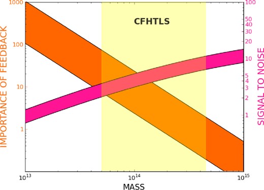
The importance of feedback (in orange) increases in systems of lower mass since the balance between the gravitational forces and the energetic processes happening in the core of galaxies (mostly linked to massive black holes) changes in favour of the latter (Giodini et al. 2010). The signal to noise of weak lensing observations (in magenta) determining how well we can measure the total mass of the system, increases for systems of larger mass. These opposite behaviours define a ‘sweet spot’ in the mass range at 1014 M⊙, where feedback is important and the mass of individual systems is measurable with weak lensing. With the CFHTLS, we can study systems exactly in this mass range (yellow shaded area).
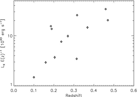
X-ray luminosity versus redshift for our cluster sample selected from XMM-CFHTLS (Mirkazemi et al. 2015).
We use lensing measurements of individual systems from the Canada–France–Hawaii Telescope Lensing Survey (CFHTLenS) and XMM–Newton X-ray observations from the XMM-CFHTLS survey. We refer to this sample as CFHTLS in this paper. This sample also includes one system from the XMM-LSS survey. We also include lower mass systems from COSMOS (Kettula et al. 2013b) and massive clusters from CCCP (Hoekstra et al. 2012; Mahdavi et al. 2013; Hoekstra et al. 2015) in order to study the mass dependence of the scaling relations. Combining the data from these three surveys allows us to constrain weak lensing calibrated scaling relations using a long mass baseline spanning approximately two orders of magnitude.
As pedagogically illustrated in appendix A of Mantz et al. (2010) scaling relations are affected by both Malmquist and Eddington bias. Both Malmquist and Eddington bias will only affect the relations in case of covariance between the intrinsic scatters of the observable used for cluster detection and the measurables under investigation. The effect of Eddington bias cannot be eliminated in the presence of intrinsic scatter about the mean relation (Eddington 1913) – because of the interplay between the steep decline at high masses of the mass function and intrinsic scatter of luminosity and temperature, it is more likely that lower mass systems scatter towards a higher luminosity or temperature, than vice versa. This renders massive clusters hotter and more luminous for their mass than intermediate-mass systems, whereas this is less of an issue for the low and intermediate-mass samples, where the mass function is flatter. In order to understand the mass dependence of the scaling relations, the effect of observational biases have to be considered. As shown by e.g. Rykoff et al. (2008) and Mantz et al. (2015), these effects can be modelled.
Clusters typically undergo several mergers during their formation, leading to a varying degree of substructure and triaxial asymmetry. As our sample contains only measurements of individual systems, we are able to study the effects of the merger and residual activity on the scaling relations by dividing our sample into subsamples of relaxed and non-relaxed systems by the amount of substructure.
Finally, galaxy cluster measurements are affected by cross-calibration uncertainties of X-ray detectors. This has been shown by the International Astronomical Consortium for High Energy Calibration IACHEC1 (Nevalainen, David & Guainazzi 2010; Kettula, Nevalainen & Miller 2013a; Schellenberger et al. 2015), and independently by e.g. Snowden et al. (2008), Mahdavi et al. (2013), Donahue et al. (2014) and Israel et al. (2015). These studies indicate that cluster temperatures measured with the Chandra observatory are typically ∼10–15 per cent higher than those measured with XMM, whereas luminosities tend to agree to a few per cent. By investigating stacked residuals, the reported discrepancies can be accounted for by differences in the energy dependence of the effective area (Kettula, Nevalainen & Miller 2013a; Read, Guainazzi & Sembay 2014; Schellenberger et al. 2015).
The lensing measurements are presented in Section 2.1 and X-ray observations in Section 2.2. We derive the lensing masses in Section 3 and present the scaling relations between lensing mass and X-ray luminosity and temperature in Section 4. We include bias corrections, and study the effects of cluster morphology and X-ray cross-calibration. Finally, we discuss our results in Section 5, and summarize our work and present our conclusions in Section 6. We denote scaling relations as Y–X, with Y as the dependent variable (y-direction) and X as the independent variable (x-direction). We assume a flat Λ cold dark matter cosmology with H0 = 72 km s−1 Mpc−1, ΩM = 0.30 and ΩΛ = 0.70. All uncertainties are at 68 per cent significance, unless stated otherwise.
2 DATA
2.1 The CFHTLenS
The CFHTLenS is based on the Canada–France–Hawaii Telescope Legacy Survey (CFHTLS), where a total area of 154 deg2 was imaged in five optical bands (u*g′r′i′z′). The data are spread over four distinct contiguous fields. The northern field W3 (∼44.2 deg2) lacks X-ray coverage, but large fractions of the three equatorial fields (W1: ∼64 deg2;W2: ∼23 deg2;W4: ∼23 deg2) were observed by XMM–Newton as part of the XMM-CFHTLS survey (Section 2.2).
The deep, multicolour data enable the determination of photometric redshifts of the sources (Hildebrandt et al. 2012) which are used to improve the precision of the lensing mass estimates by taking advantage of the redshift dependence. The i′-band data, which reach iAB = 25.5 (5σ), are used for the lensing measurements because of the excellent image quality. To determine an accurate lensing signal from these data also requires a special purpose reduction and analysis pipeline which was developed and tested by us and is described in detail in Heymans et al. (2012) and Erben et al. (2013). We discuss some of the key steps in the weak lensing analysis, but refer the interested reader to the aforementioned CFHTLenS papers for a more detailed discussion.
A critical step in the weak lensing analysis is the accurate measurement of galaxy shapes. As the CFHT data consist of multiple i′-band exposures (typically seven), the algorithm needs to be able to account for the varying point spread function (PSF) between exposures. The Bayesian fitting code lensfit (Miller et al. 2007, 2013) was used for this purpose. The resulting catalogue2 includes measurements of galaxy ellipticities, ϵ1 and ϵ2, which can be used as estimators of the shear with an inverse variance weight w. Image simulations were used to determine additional empirical shear calibration corrections, which depend on signal to noise and galaxy size. These are described in Miller et al. (2013) and Heymans et al. (2012). These papers also present a number of tests to identify residual systematics. A key test is the measurement of the correlation between the PSF orientation and the corrected galaxy shape. Heymans et al. (2012) found that 75 per cent of the data pass this test and thus can be used in the cosmological analyses (Benjamin et al. 2013; Heymans et al. 2013; Kilbinger et al. 2013; Simpson et al. 2013; Kitching et al. 2014).
Cosmic shear studies are very sensitive to such residual correlations. In this paper, however, we measure the ensemble azimuthally averaged signal around a large number of low-mass clusters. As is the case for the study of the lensing signal around galaxies (Velander et al. 2014; Hudson et al. 2015), this measurement is much more robust against residual (additive) biases. Therefore we follow Velander et al. (2014) and use all CFHTLenS fields in our analysis. Six of our clusters reside within 5 arcmin of the image edges. As the PSF varies across the field of view, it is different from the central and outer regions of a pointing. As an additional sanity check of the reliability of our cluster masses, we therefore compare the masses of these six clusters to the other ones. We do not find any systematic difference with respect to the scaling relations.
Hildebrandt et al. (2012) present measurements of the photometric redshifts for the sources using the Bayesian photometric redshift code bpz (Benítez 2000). Importantly, the PSF was homogenized between the five optical bands, which improves the accuracy of the photometric redshifts across the survey. The robustness of the photometric redshifts was tested in Hildebrandt et al. (2012) and Benjamin et al. (2013).
To ensure that robust shape measurements and reliable redshift estimates are available, we limit the source sample to those with 0.2 < zBPZ < 1.3 and i′ < 24.7. The selection yields a scatter in photometric redshift in the range 0.03 < σ < 0.06 with outlier rates smaller than 10 per cent (Hildebrandt et al. 2012). We also exclude galaxies that have the flag MASK > 0 as their photometry and shape measurement may be affected by image artefacts. The resulting sample has a weighted mean source redshift of 〈z〉 = 0.75 and an effective number density of neff = 11 arcmin−2.
2.2 The XMM-CFHTLS survey
11 clusters with X-ray flux significance greater than 20, corresponding to a minimum of 400 photons sufficient for reliable temperature measurements, have been observed by XMM–Newton as a part of the XMM-CFHTLS survey (PI: Finoguenov, see Mirkazemi et al. 2015). We also include one cluster (XID102760) from the CFHTLS W1 field which has been observed as a part of the XMM-LSS survey, with the analysis presented in Gozaliasl et al. (2014). The clusters have been identified from ROSAT All Sky Survey data, through optical filtering using CFHTLS multiband data and spectroscopic follow-up with HECTOSPEC/MMT Mirkazemi et al. (2015).
When compared to existing samples of galaxy clusters and groups, XMM-CFHTLS covers an interesting range of properties, bridging the intermediate mass range between groups and clusters. Because of the combination of a wide area with a moderately deep X-ray coverage, XMM-CFHTLS contains more low-mass systems at intermediate redshift than other XMM cluster samples such as REXCESS (Böhringer et al. 2007) or LocuSS (Smith et al. 2005), but not as low mass as those in COSMOS (Scoville et al. 2007). The typical system in XMM-CFHTLS is a low-mass cluster with a mean total mass of ∼1014 M⊙, so that we can call these Virgo-sized systems (Fig. 2).
The selection effects on the scaling relations involving other parameters than total luminosity depend on the covariance with the scatter. Since we work with core-excised temperature TX and luminosity LX, both measured inside 0.1–1 R500,3 the bias due to selection on full luminosity L can only be present if there is a covariance in the scatter between the full luminosity and core-excised TX and LX. For example if cool core clusters have slightly different properties in the outskirts, some residual bias might be present (Zhang et al. 2011). However, at present the evidence for this effect is very marginal and we have decided not to correct for it. By determining the scaling relations separately for relaxed and unrelaxed clusters, we remove the effects of such residual biases.
For calculating LX, we used the full aperture (0.1–1 R500) and the measured temperature for K-correction, reducing the scatter associated with the assumption of the shape of the emission and predicting temperatures using the LX–TX relation. As X-ray selection preferentially detects relaxed clusters (due to cool cores) and the gas distribution generally displays stronger spherical symmetry than the underlying dark matter distribution, we did not consider orientation dependence in cluster selection. As we expect the contribution from triaxiality to be minimal, we assume spherical symmetry. We study the validity of this assumption is Section 5.4.
In measuring the temperature, we only use data from the EPIC-pn instrument, and performed a local adjustment of the background in addition to the use of stored instrument background, as in Finoguenov, Böhringer & Zhang (2005) and Pratt et al. (2007), since the clusters occupy only a small part of the detector. In the spectral analysis, we used the 0.5–7.5 keV energy band, excluding the 1.4–1.6 keV interval affected by instrumental line emission. We used sas version 13.5.0 and corresponding calibration files to construct the responses.
3 WEAK LENSING SIGNAL
The differential deflection of light rays by an intervening lens leads to a shearing (and magnification) of the images of the sources (see e.g. Hoekstra et al. 2013, for a recent review on gravitational lensing studies of clusters). The resulting change in ellipticity, however, is typically much smaller than the intrinsic source ellipticity and an estimate for the shear is obtained by averaging the shapes of an ensemble of source galaxies.
Hence the redshift dependence of the lensing signal and the noise due to the intrinsic shapes of the finite number of sources, limit both the mass and redshift range for which individual cluster masses can be measured. To ensure a sufficient number density of background galaxies, we limit the analysis to clusters with z < 0.6.
As discussed in Section 2.1 we only use sources with i′ < 24.7, to ensure a robust shape measurement and we limit our sample to 0.2 < z < 1.3, to ensure the robustness of the photometric redshifts (Hildebrandt et al. 2012). To minimize the contamination of cluster members in our source sample, we consider only source galaxies with a photometric redshift larger than zlens+0.15. The redshift cut of 0.15 is a conservative one, and results in negligible contamination of cluster galaxies in the source sample. Including sources even closer to the lens redshift would not lead to a large improvement in signal to noise, as their lensing efficiencies are small. As the redshifts of our clusters are <0.6, the photo-z errors of the sources are almost flat close to the lens redshift (Hildebrandt et al. 2012), and the photo-z cut needs not be redshift dependent.
Analytic expressions for the tangential shear of NFW profiles have been derived by Wright & Brainerd (2000) and Bartelmann (1996). We fit the NFW model shear to the profiles shown in Fig. 3 and indicate the best-fitting model by the solid line. The coloured region indicates the 68 per cent region for the model. As we measure M200 from the NFW profile using the mass–concentration relation in equation (10), we have one free parameter for 15 radial bins giving 14 degrees of freedom (we note that cluster XID210640 falls in the middle of a large stellar halo mask and lacks data on smaller scales). We test the best-fitting NFW profile against the null hypothesis that the tangential shear signal is zero and show the reduced χ2 values in Fig. 3. We use the best-fitting NFW profile to rescale virial mass to M500. The resulting values for M200 and M500 are listed in Table 1.
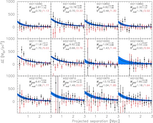
Shear profiles out to 3 Mpc for the individual X-ray clusters measured using CFHTLenS data that were detected with an X-ray flux significance higher than 20, corresponding to a minimum of 400 photons. The blue shaded line shows the uncertainty on the best-fitting profile. Each panel shows the mass M200 and the error of the mass in units of 1014 M⊙, measured shear profiles and the χ2 values for the NFW profile fit to the tangential shear (black circles). The cross-shear and the χ2 value of the null hypothesis that the tangential shear signal is zero are shown in red. Cluster XID210640 falls in the middle of a large stellar halo mask and lacks data on smaller scales.
Table of X-ray measurements and weak lensing masses for systems in our sample.
| XID | RA | DEC | z | LX | TX | M200 | M500 | DBCG |
|---|---|---|---|---|---|---|---|---|
| (deg) | (deg) | (1043 erg s−1) | (keV) | (1014 M⊙) | (1014 M⊙) | (kpc) | ||
| 110090 | 36.2713 | −9.8381 | 0.159 | 3.16 ± 0.18 | 3.62 ± 0.79 | |$2.81^{+1.79}_{-1.42}$| | |$2.00^{+1.28}_{-1.02}$| | 17 |
| 110460 | 35.998 | −8.5956 | 0.27 | 11.19 ± 0.71 | 7.25 ± 3.19 | |$10.78^{+4.08}_{-3.44}$| | |$7.45^{+2.82}_{-2.38}$| | 28 |
| 110850 | 33.6064 | −6.4605 | 0.237 | 8.52 ± 0.35 | 2.39 ± 0.7 | |$4.82^{+2.48}_{-1.98}$| | |$3.38^{+1.74}_{-1.39}$| | 17 |
| 110860 | 36.3021 | −6.3837 | 0.204 | 4.0 ± 0.28 | 3.87 ± 1.19 | |$2.30^{+1.76}_{-1.31}$| | |$1.64^{+1.26}_{-0.93}$| | 13 |
| 111180 | 37.9269 | −4.8814 | 0.185 | 16.90 ± 0.37 | 5.0 ± 0.61 | |$11.81^{+3.11}_{-2.67}$| | |$8.23^{+2.17}_{-1.86}$| | 62 |
| 210010 | 133.0656 | −5.5651 | 0.189 | 14.94 ± 0.29 | 4.88 ± 0.62 | |$9.92^{+3.30}_{-2.82}$| | |$6.93^{+2.31}_{-1.97}$| | 24 |
| 210020 | 134.6609 | −5.4211 | 0.1 | 1.56 ± 0.08 | 1.65 ± 0.3 | |$1.06^{+1.32}_{-0.88}$| | |$0.77^{+0.96}_{-0.64}$| | 431 |
| 210630 | 133.5554 | −2.3499 | 0.368 | 17.53 ± 0.98 | 5.31 ± 2.48 | |$3.52^{+5.67}_{-3.50}$| | |$2.45^{+3.95}_{-2.44}$| | 29 |
| 210740 | 135.4147 | −1.9799 | 0.314 | 4.04 ± 0.22 | 4.59 ± 1.57 | |$6.61^{+3.54}_{-2.84}$| | |$4.58^{+2.45}_{-1.97}$| | 21 |
| 210910 | 135.3770 | −1.6532 | 0.316 | 29.95 ± 1.56 | 5.04 ± 2.42 | |$12.94^{+7.72}_{-6.10}$| | |$8.87^{+5.29}_{-4.18}$| | 30 |
| 210970 | 133.0675 | −1.0260 | 0.459 | 42.81 ± 1.07 | 5.35 ± 1.18 | |$13.72^{+8.17}_{-6.09}$| | |$9.25^{+5.50}_{-4.10}$| | 42 |
| 102760 | 35.4391 | −3.7712 | 0.47 | 25.88 ± 1.13 | 8.2 ± 5.55 | |$7.80^{+5.38}_{-3.97}$| | |$5.30^{+3.66}_{-2.70}$| | 32 |
Notes. XID is the X-ray identification number in the XMM-CFHTLS survey, RA and DEC are the coordinates of the cluster centre defined by the X-ray peak, z the redshift of the cluster, TX and LX the X-ray temperature and luminosity, M200 and M500 the spherical overdensity masses with respect to the critical density and DBCG the offset between the BCG and X-ray peak.
These are indeed the most massive clusters in the XMM-CFHTLS data, but the observed lensing signal is nevertheless quite sensitive to contributions from uncorrelated large-scale structure along the line of sight (Hoekstra 2001; Hoekstra et al. 2011) or substructure and triaxial shape of the cluster halo (Corless & King 2007; Meneghetti et al. 2010; Becker & Kravtsov 2011). Such structures modify the observed tangential shear profile. Both effects are an additional source of noise, whereas the latter might lead to biased mass estimate if we fit an NFW model to the data.
The χ2 values of the NFW profile fits shown in Fig. 3 show that the data are well described by a single NFW profile. However, we note that for XID210910 a secondary group is detected in the X-ray image, which would tend to bias the NFW mass high.
3.1 Systematics in mass estimates
The accuracy of the scaling relations depends on the ability to measure unbiased cluster masses. In this section, we investigate different systematic effects that can bias our lensing masses.
As we fit the density profiles down to a radial range of 150 kpc, the resulting masses can be affected by the mass–concentration relation assumed for the NFW profile. This was explored by Hoekstra et al. (2012), who showed that the sensitivity to the mass–concentration depends on the fit range and overdensity Δ. They found their masses using a fit range of 0.5–2.0 Mpc to be most stable with Δ = 1000. To investigate how sensitive our masses are to the selected mass–concentration relation, we fit the NFW profiles assuming the relation of Dutton & Macciò (2014). We find that the average ratio of best-fitting masses using Dutton & Macciò (2014) to Duffy et al. (2008) is 0.92 ± 0.04, i.e. Dutton & Macciò (2014) results on average in lower masses by 2σ (see Fig. 4). As an additional test, we also measured our masses by excluding the central 0.5 Mpc and find perfect agreement with our reported mass estimates. The average ratio of best-fitting masses is 0.99 ± 0.11 (see Fig. 4).
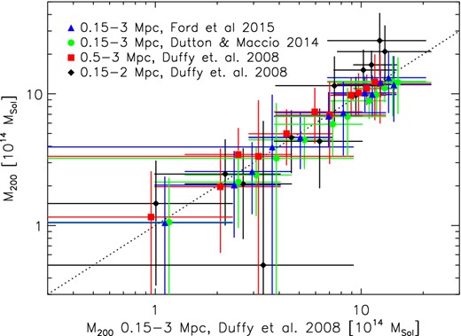
Comparison of mass measurements assuming different mass–concentration relations, radial fit ranges or background galaxy filtering to the mass measurements adopted in this work.
Simulations by Becker & Kravtsov (2011) suggest that extending the fit range beyond the virial radius may bias lensing masses low by 5–10 per cent due to the correlated large-scale structure. To test this, we adopt an upper fit range of 2 Mpc. In this case, we find that the average ratio of the best-fitting masses is 1.15 ± 0.49. If fitting beyond the virial radius would bias our mass estimates low, the ratio of the best-fitting masses should be larger for low-mass systems with smaller virial radii than for massive clusters. We are not able to detect this trend in the data (see Fig. 4).
In the lensing measurement, we compute the mean lensing efficiency 〈Dls/Ds〉 for each source by integrating over the full stacked photo-z posterior probability distribution P(z). Since the relation between lensing efficiency and redshift is non-linear, this could introduce a bias if the stacked P(z) is not a fair representation of the actual redshift distribution of the sources. To estimate its size, we consider a single lens–source pair. For the lens, we adopt a redshift of 0.2. For the source, we assume a redshift probability distribution that is representative for objects in CFHTLenS (see Hildebrandt et al. 2012), i.e. we describe the stacked P(z) by a Gaussian with a mean of 0.7 and a standard deviation of 0.05, plus a second Gaussian with a standard deviation of 0.5 (but with the same mean) that contains 7 per cent of the total probability, to account for an outlier fraction of 7 per cent. We compare the input Dls/Ds to the one that is averaged over the stacked P(z), and find that the latter is biased low by 1 per cent. Repeating the test for a lens at a redshift of 0.5 and a mean source redshift of 0.9, we find a similar bias.
If not properly accounted for, dilution by foreground galaxies can bias the mass measurements. Using the P(z) modelling above, we compute a mass dilution by foreground galaxies of 3.5 per cent. As a final test, we re-measure the masses using the same selection criteria for background galaxies as Ford et al. (2015), i.e. that the peak of the galaxy's P(z) is higher than the redshift of the cluster and that at least 90 per cent of the galaxy's P(z) is at a higher redshift than the cluster. In this case, we find that the best-fitting masses are consistent with our measurements, with an average ratio of 0.97 ± 0.08 (see Fig. 4). We also note that in case our mass measurements would be significantly diluted by foreground galaxies, the expected ratio would be higher than unity.
4 SCALING RELATIONS
The combination of X-ray and CFHTLenS weak lensing data is ideal for calibrating cluster mass proxies in the low-mass cluster regime. We present our fitting method, sample, bias corrections, and morphological classification of systems in Section 4.1. In Sections 4.2, 4.3 and 4.4, we present the scaling between weak lensing mass, core-excised X-ray luminosity and temperature,and discuss the global scaling properties (we explore the mass and morphology dependence of the relations in Sections 5.3 and 5.4). Finally, we study the effects of X-ray cross-calibration in 4.5.
4.1 Fitting method
We let both the slope α, normalization log10(N) and intrinsic scatter σlog (A|B) vary freely in the fits. We use the Bayesian linear regression routine of Kelly (2007) with the Metropolis–Hastings sampler to find the best-fitting parameters. The routine includes intrinsic scatter in the dependent variable (i.e. y-direction) σlog (A|B), which we expect to follow a lognormal distribution. We define best-fitting parameters as the median of the single parameter posterior distributions and errors as the values corresponding to the 68th percentiles.
In order to improve the precision and to study the mass dependence of the relation, we include measurements of 10 individual low-mass systems from the Cosmic Evolution Survey (COSMOS) and 48 individual high-mass systems from the Canadian Cluster Comparison Project (CCCP). We utilize the three surveys making up our sample as overlapping mass bins, with COSMOS forming the low-mass, CFHTLS intermediate-mass and CCCP the high-mass bin, and fit the scaling relations independently for each of the surveys.
COSMOS data, lensing and temperature measurements are presented in Kettula et al. (2013b). The COSMOS systems have lensing masses based on deep HST imaging and 30+ band photometric redshifts, and X-ray measurements obtained with XMM–Newton. We derive luminosities from the COSMOS data using the method presented in Section 2.2 in this work (see Table A1). For the CCCP sample, we use recent lensing mass measurements presented in Hoekstra et al. (2015) measured assuming an NFW density profile and the Duffy et al. (2008) mass–concentration relation and X-ray measurements obtained with both Chandra and XMM–Newton. We derive core-excised LX using the 0.1–2.4 keV band for the CCCP systems using the method described in Mahdavi et al. (2013, see also Mahdavi et al. 2014) and use the core-excised temperatures from Mahdavi et al. (2013).4 The soft band LX measurements are given in Table A2. Chandra observations of CCCP clusters are adjusted to match XMM–Newton calibration. This gives us a sample of 72 individual systems, with TX ∼ 1–12 keV, LX ∼1043–1045 erg s−1 and a mass from ∼1013 to a few times 1015 M⊙.
We note that there are differences in the calibration of the lensing signal for these additional data sets, compared to CFHTLS. Furthermore, the CCCP data lack photometric redshift information which may impact the correction for contamination by cluster members. These uncertainties impact the masses at the 5–10 per cent level for individual clusters. We estimated the effect of the lensing calibration uncertainties by examining how the slopes of M–TX and M–LX relations change when decreasing the mass of all COSMOS systems by 5 per cent while increasing CCCP masses by 5 per cent and vice versa. We find that the effect is small at 3 and 5 per cent for M–TX and M–LX and do not include this effect in the quoted statistical uncertainties.
4.1.1 Bias correction
The Kelly (2007) regression method attempts to correct for sampling effects in the independent variable (x-direction). Since we deal with X-ray selected samples of galaxy clusters, we are thus able to correct for possible residual Malmquist bias due to the covariance between the studied parameter and the parameter used to select the clusters by keeping LX or TX as the independent variable. However, the regression method determines the scatter only for the dependent variable, and assumes no intrinsic scatter for the independent variable. Consequently, we first have to determine the scatter in LX and TX at fixed mass and add these to the statistical errors.
Therefore we first measure the global inverted relation with mass as the independent variable to determine the scatter in LX and TX. We assume that the intrinsic scatter of mass measurement using weak lensing with respect to the true mass is 0.2 in natural logarithm units (Becker & Kravtsov 2011), and add this value to the mass errors for every fit having mass as the independent variable. As shown by Vikhlinin et al. (2009), the value of the scatter is independent of a possible bias in the slope.
For total scatter in LX and TX, we use the summed square of the statistical errors and measured intrinsic scatter. The value for the total scatter in weak lensing masses, which correspond to the a convolution of the data quality and the intrinsic scatter, is assumed to be 0.3 in natural logarithm units. This value is used both as the total scatter term for mass and to smooth the theoretical mass function to establishing the derivative of the distribution of clusters as a function of weak lensing mass. Using weak lensing mass as opposed to the true mass yields smaller slopes for the mass function.
We refer to the measurements corrected for Eddington bias and scaling relations fitted to the corrected measurements as bias corrected (BC). The bias correction is discussed in more detail in Leauthaud et al. (2010). Contrary to Leauthaud et al. (2010), who used the global slope of the mass function, we use a local one for each system. In both cases we implicitly assume a strong covariance between the selection and observable. While both methods lead to small global changes, using the local slope leads to sizeable corrections in particular for the CCCP sample, which contains a large number of massive clusters at relatively high redshifts. We show the bias corrections for individual systems in Fig. 5 and list them in Appendix B.
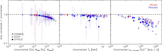
The values of the Eddington bias corrections applied to mass (left-hand panel), temperature (middle panel) and luminosity (right-hand panel). Blue and red dotted data show the residuals for individual merging and relaxed systems, squares indicate systems from COSMOS, circles from CCCP and solid diamonds from CFHTLS. Errors are the statistical errors of the measurements.
As the Kelly (2007) fitting routine corrects for Malmquist bias in the independent variable, our bias-corrected M–LX and M–TX relations are fully corrected for observational biases, whereas there might be some residual covariance affecting the LX–M, TX–M and LX–TX relations. However, we expect the effect for the global relation to be small. We also explored fits performed individually for each survey (accounting separately for Malmquist bias) and combining the posterior distributions, but found that the combined posterior not to be as constraining as the combined data set.
4.1.2 Morphological classification
The distance between the brightest cluster galaxy (BCG) and X-ray surface brightness peak (DBCG) has been shown to be a good indicator of the relaxation state by e.g. Poole et al. (2007) and Mahdavi et al. (2013). Large values for DBGC indicate significant substructure typical for unrelaxed clusters. We are able to identify BCG locations using the XMM-CFHTLS optical photometry of Mirkazemi et al. (2015). For the XMM-LSS cluster XID102760, we use photometry of Gozaliasl et al. (2014). The location of the X-ray peaks are determined from X-ray photometry presented in this work. For COSMOS and CCCP systems, we use DBCG values presented in Kettula et al. (2013b) and Mahdavi et al. (2013), respectively.
We classify clusters with DBGC < 3 per cent of R200 as relaxed and those with DBGC ≥ 3 per cent of R200 as non-relaxed (which we refer to as mergers or merging clusters). Here, R200 is the radius inside which the mean density of the cluster corresponds to 200 times the critical density at the redshift of the system. For our sample, 3 per cent of R200 corresponds to 13–75 kpc and gives 55 relaxed systems and 15 non-relaxed merging systems (see Fig. 6). As the CFHTLS and COSMOS samples are selected on X-ray brightness and the CCCP sample, though originally selected on ASCATX, is consistent with well-defined flux-based samples (Mahdavi et al. 2013), we expect to find a large fraction of relaxed clusters with cool cores associated with high X-ray brightness peaks.
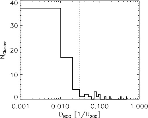
The distribution of offsets between X-ray peak and BCG DBGC. DBGC are given as fractions of R200. The dotted vertical line separates between relaxed and merging clusters.
4.2 LX–TX relation
For the LX–TX relation, we adopt L0 = 1044 erg s−1 and T0 = 5 keV. The resulting relations and fit parameters are shown in Figs 7 –9, and Table 2.
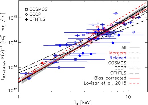
The scaling of core-excised X-ray temperature TX to core-excised luminosity LX. The black solid line and grey shaded region shows the best-fitting relation and statistical uncertainty fitted to all data, the red solid line shows the corresponding BC relation. The dotted line shows the relation fitted to relaxed clusters (blue data) and dashed line to merging clusters (red data). The dot–dashed and long dashed lines shows relations fitted independently to each survey and the red dashed line is the best-fitting uncorrected relation from Lovisari et al. (2015). Errors on data indicate statistical uncertainties.
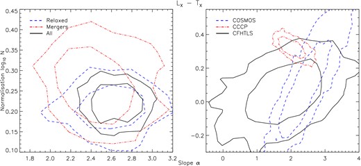
Confidence contours for the posterior distributions of slope and normalization at 68 and 95 per cent significance for the LX–TX relations fitted to each respective subsample.
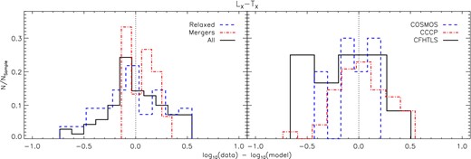
The distribution of residuals for each subsample with respect to the LX–TX relation fitted to the full sample. NSample is defined as the number of systems in each subsample.
The fit parameters and intrinsic scatter with the corresponding statistical uncertainties of the scaling relations.
| α | log10N | |$\sigma _{\rm \log (A|B)}$| | |
|---|---|---|---|
| LX–TX | |||
| All data | |$2.65^{+0.17}_{-0.17}$| | |$0.23^{+0.03}_{-0.03}$| | |$0.15^{+0.04}_{-0.04}$| |
| Bias corrected | |$2.52^{+0.17}_{-0.16}$| | |$0.18^{+0.03}_{-0.03}$| | |$0.10^{+0.04}_{-0.04}$| |
| Mergers | |$2.46^{+0.27}_{-0.24}$| | |$0.27^{+0.06}_{-0.06}$| | |$0.10^{+0.07}_{-0.05}$| |
| Relaxed | |$2.62^{+0.22}_{-0.22}$| | |$0.21^{+0.04}_{-0.04}$| | |$0.20^{+0.05}_{-0.04}$| |
| CFHTLS | |$1.84^{+0.80}_{-0.76}$| | |$0.06^{+0.12}_{-0.13}$| | |$0.34^{+0.13}_{-0.09}$| |
| COSMOS | |$2.40^{+0.54}_{-0.46}$| | |$0.08^{+0.21}_{-0.19}$| | |$0.17^{+0.12}_{-0.09}$| |
| CCCP | |$2.06^{+0.29}_{-0.28}$| | |$0.32^{+0.04}_{-0.04}$| | |$0.13^{+0.04}_{-0.04}$| |
| LX–M200 | |||
| All data | |$1.13^{+0.10}_{-0.10}$| | |$-0.22^{+0.06}_{-0.06}$| | |$0.33^{+0.03}_{-0.03}$| |
| Bias corrected | |$1.27^{+0.16}_{-0.15}$| | |$-0.38^{+0.06}_{-0.06}$| | |$0.29^{+0.04}_{-0.03}$| |
| M200–LX | |||
| All data | |$0.74^{+0.08}_{-0.08}$| | |$0.31^{+0.04}_{-0.04}$| | |$0.15^{+0.04}_{-0.04}$| |
| Bias corrected | |$0.74^{+0.09}_{-0.08}$| | |$0.40^{+0.03}_{-0.03}$| | |$0.10^{+0.04}_{-0.04}$| |
| Mergers | |$0.60^{+0.16}_{-0.15}$| | |$0.29^{+0.10}_{-0.11}$| | |$0.21^{+0.10}_{-0.09}$| |
| Relaxed | |$0.78^{+0.09}_{-0.09}$| | |$0.31^{+0.04}_{-0.05}$| | |$0.14^{+0.04}_{-0.04}$| |
| CFHTLS | |$0.66^{+0.35}_{-0.29}$| | |$0.47^{+0.09}_{-0.10}$| | |$0.15^{+0.12}_{-0.08}$| |
| COSMOS | |$0.83^{+0.46}_{-0.39}$| | |$0.35^{+0.37}_{-0.34}$| | |$0.28^{+0.21}_{-0.13}$| |
| CCCP | |$0.80^{+0.38}_{-0.29}$| | |$0.25^{+0.15}_{-0.21}$| | |$0.17^{+0.04}_{-0.05}$| |
| M500–LX | |||
| All data | |$0.70^{+0.08}_{-0.07}$| | |$0.15^{+0.04}_{-0.04}$| | |$0.14^{+0.03}_{-0.03}$| |
| TX–M500 | |||
| All data | |$0.45^{+0.04}_{-0.04}$| | |$-0.02^{+0.02}_{-0.02}$| | |$0.11^{+0.01}_{-0.01}$| |
| Bias corrected | |$0.48^{+0.06}_{-0.06}$| | |$-0.03^{+0.02}_{-0.02}$| | |$0.06^{+0.02}_{-0.02}$| |
| M500–TX | |||
| All data | |$1.68^{+0.17}_{-0.17}$| | |$0.08^{+0.03}_{-0.03}$| | |$0.14^{+0.03}_{-0.03}$| |
| Bias corrected | |$1.52^{+0.17}_{-0.16}$| | |$0.05^{+0.03}_{-0.03}$| | |$0.07^{+0.04}_{-0.03}$| |
| Mergers | |$1.43^{+0.32}_{-0.31}$| | |$0.05^{+0.07}_{-0.07}$| | |$0.18^{+0.09}_{-0.07}$| |
| Relaxed | |$1.78^{+0.22}_{-0.21}$| | |$0.09^{+0.03}_{-0.04}$| | |$0.15^{+0.04}_{-0.04}$| |
| CFHTLS | |$1.34^{+0.78}_{-0.73}$| | |$0.14^{+0.09}_{-0.10}$| | |$0.16^{+0.13}_{-0.08}$| |
| COSMOS | |$1.52^{+0.90}_{-0.82}$| | |$-0.14^{+0.34}_{-0.34}$| | |$0.29^{+0.21}_{-0.14}$| |
| CCCP | |$1.18^{+0.31}_{-0.29}$| | |$0.14^{+0.05}_{-0.05}$| | |$0.17^{+0.03}_{-0.03}$| |
| M200–TX | |||
| All data | |$1.73^{+0.19}_{-0.17}$| | |$0.26^{+0.03}_{-0.03}$| | |$0.15^{+0.03}_{-0.03}$| |
Notes. α is the slope of the relation, log10N the normalization and |$\sigma _{\rm \log (A|B)}$| the intrinsic scatter. BC relations are fitted to the full data set.
The scatter in LX at fixed temperature is |$0.15^{+0.04}_{-0.04}$| for the uncorrected relation and |$0.10^{+0.04}_{-0.04}$| for the BC relation. The slopes are steeper than the self-similar prediction of 2.0, we get |$2.65^{+0.17}_{-0.17}$| in the uncorrected case and |$2.52^{+0.17}_{-0.16}$| after bias correction.
Lovisari et al. (2015) used XMM–Newton observations of a flux-limited set of nearby galaxy groups together with data of the HIFLUGCS clusters from Hudson et al. (2010), resulting in a sample spanning a similar LX and TX range as ours. In Fig. 7, we compare their relation corrected for selection bias effects (using full luminosities and core-excised temperatures) to our core-excised relations. We find that their slope is consistent within the uncertainties with our relation, but they predict systematically higher luminosities at fixed temperature because they use total luminosities.
4.3 M–LX relation
X-ray luminosity LX is the observationally cheapest X-ray observable, requiring only source detection and redshift information for its measurement. Luminosity is hence the mass proxy choice for shallow X-ray surveys, making the mass–luminosity relation potentially a powerful cosmological instrument.
As typically done in the literature, we opt to study the scaling of luminosity to the total mass of the halo given by M200, (but also quote the parameters for scaling to M500). For the M–LX relations, we set L0 to 1044 erg s−1 and M0 to 3 × 10¹⁴ M⊙. The resulting relations and fit parameters are shown in Figs 10–12 and Table 2.
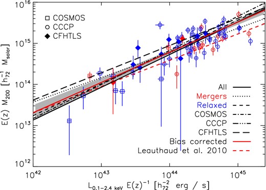
The scaling of mass M200 to core-excised luminosity LX. The black solid line and grey shaded region shows the best-fitting relation and statistical uncertainty fitted to all data, the red solid line shows the corresponding BC relation. The dotted line shows the relation fitted to relaxed clusters (blue data) and dashed line to merging clusters (red data). The dot–dashed and long dashed lines shows relations fitted independently to each survey and the red dashed line is the best-fitting uncorrected relation from Leauthaud et al. (2010). Errors on data indicate statistical uncertainties.
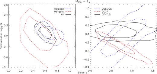
Confidence contours for the posterior distributions of slope and normalization at 68 and 95 per cent significance for the M200–LX relations fitted to each respective subsample.
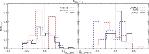
The distribution of residuals for each subsample with respect to the M200–LX relation fitted to the full sample. NSample is defined as the number of systems in each subsample.
The scatter in LX at fixed mass is |$0.33^{+0.03}_{-0.03}$| in the uncorrected case and |$0.29^{+0.04}_{-0.03}$| in the BC case. We obtain a consistent slope for the BC and uncorrected relations, the uncorrected slope is |$0.74^{+0.08}_{-0.08}$|. The slope is consistent with the purely gravitational self-similar prediction of 0.75.
Currently the only other M–LX relation spanning a similar mass range as ours using weak lensing mass calibration is that of Leauthaud et al. (2010). They derived non-core excised luminosities and lensing masses for stacked low-mass galaxy groups in the COSMOS field and combined them with higher mass systems from the literature. Their slope of 0.64 ± 0.03 is flatter than ours. The Leauthaud et al. (2010) relation predicts consistent luminosities with us at low masses, but leading to significant tension at high masses (see Fig. 10). In addition to the weak lensing measurements, the mass calibration of the low-mass Leauthaud et al. (2010) sample has been confirmed by magnification analysis (Ford et al. 2012; Schmidt et al. 2012) and clustering (Allevato et al. 2012).
4.4 M–TX relation
The relation between mass and temperature is the most fundamental among the scaling relations because it provides the physical link between X-ray observations of galaxy clusters and the models of structure formation. If the only source of heating of the gas is gravitational and there is no efficient cooling, the gas temperature is a direct measure of the potential depth, and therefore of the total mass.
For the M–TX relation, we opt to study the scaling to M500, as is usually done in the literature (but we also quote the parameters of the relation for M200). The best-fitting relations and fit parameters for M0 = 5 × 10¹⁴ M⊙ and T0 = 5.0 keV are shown in Figs 13–15 and Table 2.
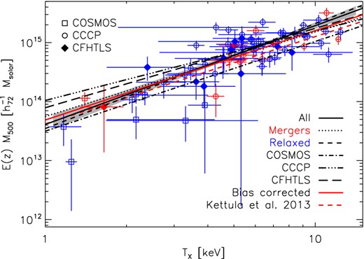
The scaling of mass M500 to core-excised temperature TX. The black solid line and grey shaded region shows the best-fitting relation and statistical uncertainty fitted to all data, the red solid line shows the corresponding BC relation. The dotted line shows the relation fitted to relaxed clusters (blue data) and dashed line to merging clusters (red data). The dot–dashed and long dashed lines shows relations fitted independently to each survey and the red dashed line is the best-fitting uncorrected relation from Kettula et al. (2013b). Errors on data indicate statistical uncertainties.
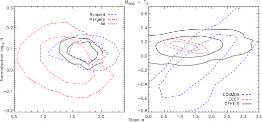
Confidence contours for the posterior distributions of slope and normalization at 68 and 95 per cent significance for the M500–TX relations fitted to each respective subsample.
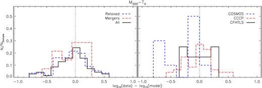
The distribution of residuals for each subsample with respect to the M500–TX relation fitted to the full sample. NSample is defined as the number of systems in each subsample.
We find that TX is a low-scatter mass proxy, the intrinsic scatter in temperature at fixed mass is |$0.11^{+0.01}_{-0.01}$| in the uncorrected case and |$0.06^{+0.02}_{-0.02}$| for the fully BC relation. The slope of the uncorrected relation is |$1.68^{+0.17}_{-0.17}$|. The bias correction results in a slightly shallower slope of |$1.52^{+0.17}_{-0.16}$|, which is fully consistent with the self-similar prediction of 1.50.
In Fig. 13, we also compare our relations to the best-fitting M–TX relation from Kettula et al. (2013b), where we use CCCP with different temperature measurements as a high-mass sample and five clusters from the 160 Square Degree survey as an intermediate-mass sample to infer a scaling consistent the self-similarity. We find that the best-fitting relation of Kettula et al. (2013b) has a shallower slope than our uncorrected and BC relations, predicting somewhat lower temperatures for a given mass in the high-mass end.
4.5 X-ray cross-calibration
We investigated the effects of cross-calibration on scaling relations by modifying our XMM-based temperatures and luminosities to match Chandra calibration, allowing direct comparison to relations measured with Chandra. We modified our temperatures using the best-fitting relations for the full energy band by equation (3). and table 2 in Schellenberger et al. (2015). For CFHTLS and COSMOS which are measured with pn only, we used the ACIS–pn relation. For CCCP which uses all three XMM-EPIC detectors (pn, MOS1 and MOS2), we used the values for ACIS-combined XMM.
Nevalainen et al. (2010) found that Chandra results on average in ∼2 per cent higher fluxes in the soft energy band (0.5–2.0 keV) and ∼11 per cent higher in the hard band (2.0–7.0 keV) than pn. As fluxes are directly related to luminosity, any discrepancy in measured fluxes applies directly to luminosities. Mahdavi et al. (2013) reported ∼3 per cent higher bolometric luminosities for Chandra than for combined XMM. As we measure luminosities in a 0.1–2.4 keV band, we increased our XMM-based luminosities by 2 per cent in order to match the Chandra calibration.
The best-fitting parameters of the scaling relations fitted to our modified XMM data are given in Table 3, and show the relations in Figs 16–18. As expected from the small modification to luminosities, we find that modifying luminosities does not affect the resulting relations. However, modifying temperatures drives the slopes of the LX–TX and M500–TX relations to flatter values. The flattening of the slopes of the bias-corrected LX–TX and M500–TX relations are 0.35 ± 0.16 and 0.23 ± 0.15, respectively.
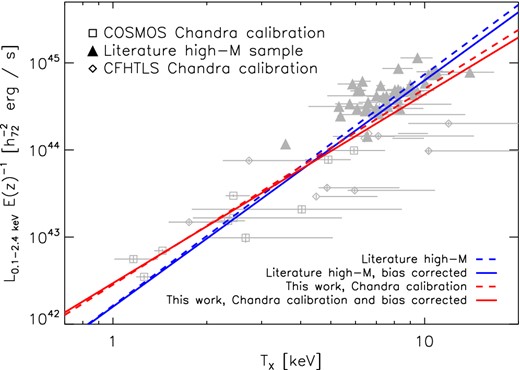
Comparison of LX–TX relations using different high-mass samples, blue lines show relations using the literature sample, red lines using CCCP converted to Chandra calibration. Solid lines show the BC relations, dashed lines the uncorrected lines. The high-mass samples are combined with COSMOS and CFHTLS data converted to Chandra calibration. COSMOS and CFHTLS data converted to Chandra calibration and measurements of the literature high-mass sample are shown in grey.
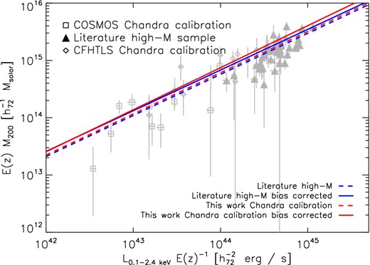
Comparison of M–LX relations using different high-mass samples, blue lines show relations using the literature sample, red lines using CCCP converted to Chandra calibration. Solid lines show the BC relations, dashed lines the uncorrected lines. The high-mass samples are combined with COSMOS and CFHTLS data converted to Chandra calibration. COSMOS and CFHTLS data converted to Chandra calibration and measurements of the literature high-mass sample are shown in grey.
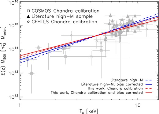
Comparison of M–TX relations using different high-mass samples, blue lines show relations using the literature sample, red lines using CCCP converted to Chandra calibration. Solid lines show the BC relations, dashed lines the uncorrected lines. The high-mass samples are combined with COSMOS and CFHTLS data converted to Chandra calibration. COSMOS and CFHTLS data converted to Chandra calibration and measurements of the literature high-mass sample are shown in grey.
The fit parameters and intrinsic scatter with the corresponding statistical uncertainties of the scaling relations with XMM temperatures and luminosities modified to match Chandra calibration.
| α | log10N | |$\sigma _{\rm \log (A|B)}$| | |
|---|---|---|---|
| LX–TXChandra calibration | |||
| All data | |$2.25^{+0.15}_{-0.15}$| | |$0.02^{+0.04}_{-0.04}$| | |$0.20^{+0.04}_{-0.03}$| |
| Bias corrected | |$2.17^{+0.15}_{-0.13}$| | |$-0.01^{+0.03}_{-0.03}$| | |$0.13^{+0.04}_{-0.04}$| |
| M200–LXChandra calibration | |||
| All data | |$0.72^{+0.08}_{-0.07}$| | |$0.31^{+0.04}_{-0.04}$| | |$0.15^{+0.03}_{-0.03}$| |
| Bias corrected | |$1.29^{+0.14}_{-0.13}$| | |$-0.07^{+0.03}_{-0.03}$| | |$0.08^{+0.04}_{-0.04}$| |
| M500–TXChandra calibration | |||
| All data | |$1.44^{+0.15}_{-0.15}$| | |$-0.05^{+0.04}_{-0.04}$| | |$0.16^{+0.03}_{-0.03}$| |
| Bias corrected | |$1.29^{+0.14}_{-0.13}$| | |$-0.07^{+0.03}_{-0.03}$| | |$0.08^{+0.04}_{-0.04}$| |
Notes. α is the slope of the relation, log10N the normalization and |$\sigma _{\rm \log (A|B)}$| the intrinsic scatter. BC relations are fitted to the full data set.
| α | log10N | |$\sigma _{\rm \log (A|B)}$| | |
|---|---|---|---|
| LX–TX literature high-mass sample | |||
| All data | |$2.65^{+0.18}_{-0.18}$| | |$0.07^{+0.04}_{-0.04}$| | |$0.18^{+0.04}_{-0.04}$| |
| Bias corrected | |$2.60^{+0.10}_{-0.13}$| | |$0.02^{+0.03}_{-0.05}$| | |$0.09^{+0.05}_{-0.04}$| |
| M200–LX literature high-mass sample | |||
| All data | |$0.72^{+0.07}_{-0.06}$| | |$0.28^{+0.04}_{-0.04}$| | |$0.08^{+0.04}_{-0.04}$| |
| Bias corrected | |$0.71^{+0.08}_{-0.08}$| | |$0.35^{+0.03}_{-0.03}$| | |$0.07^{+0.03}_{-0.03}$| |
| M500–TX literature high-mass sample | |||
| All data | |$1.76^{+0.19}_{-0.18}$| | |$-0.05^{+0.04}_{-0.04}$| | |$0.15^{+0.03}_{-0.03}$| |
| Bias corrected | |$1.56^{+0.19}_{-0.17}$| | |$-0.05^{+0.03}_{-0.03}$| | |$0.07^{+0.03}_{-0.03}$| |
Notes. α is the slope of the relation, log10N the normalization and |$\sigma _{\rm \log (A|B)}$| the intrinsic scatter. The relations are fitted to a combination of COSMOS and CFHTLS data corrected to match Chandra calibration and the literature high-mass sample.
| α | log10N | |$\sigma _{\rm \log (A|B)}$| | |
|---|---|---|---|
| LX–TX literature high-mass sample | |||
| All data | |$2.65^{+0.18}_{-0.18}$| | |$0.07^{+0.04}_{-0.04}$| | |$0.18^{+0.04}_{-0.04}$| |
| Bias corrected | |$2.60^{+0.10}_{-0.13}$| | |$0.02^{+0.03}_{-0.05}$| | |$0.09^{+0.05}_{-0.04}$| |
| M200–LX literature high-mass sample | |||
| All data | |$0.72^{+0.07}_{-0.06}$| | |$0.28^{+0.04}_{-0.04}$| | |$0.08^{+0.04}_{-0.04}$| |
| Bias corrected | |$0.71^{+0.08}_{-0.08}$| | |$0.35^{+0.03}_{-0.03}$| | |$0.07^{+0.03}_{-0.03}$| |
| M500–TX literature high-mass sample | |||
| All data | |$1.76^{+0.19}_{-0.18}$| | |$-0.05^{+0.04}_{-0.04}$| | |$0.15^{+0.03}_{-0.03}$| |
| Bias corrected | |$1.56^{+0.19}_{-0.17}$| | |$-0.05^{+0.03}_{-0.03}$| | |$0.07^{+0.03}_{-0.03}$| |
Notes. α is the slope of the relation, log10N the normalization and |$\sigma _{\rm \log (A|B)}$| the intrinsic scatter. The relations are fitted to a combination of COSMOS and CFHTLS data corrected to match Chandra calibration and the literature high-mass sample.
5 DISCUSSION
Measurements of a large number of clusters from a wide mass range are needed to gain precise constraints on scaling relations. A large spread in mass improves the constraint on the slope of the scaling and as lensing mass measurements have an intrinsic scatter of ∼20–30 per cent (e.g. Becker & Kravtsov 2011), several systems in each mass range and a good understanding of systematic uncertainties and observational biases are needed to accurately recover the average relation.
With the inclusion of the 12 low-mass clusters analysed in this work, we have more than doubled the number of systems at low and intermediate masses available in the sample used for lensing calibrated scaling relations. Previously the only individual low-mass systems with lensing and X-ray measurements were 10 groups from the COSMOS field, which extend to a larger redshift and thus possibly affected by evolutionary effects (e.g. Jee et al. 2011). On the other hand, there are extensive recent and ongoing observational efforts to obtain mass calibration for massive clusters by e.g. LoCuSS (Okabe et al. 2010), CCCP (Mahdavi et al. 2013) and Weighing the Giants (WtG; von der Linden et al. 2014a).
The systems analysed in this work increase the statistical power of the low-mass end and thus improve the precision of the constraint. In addition, we include a correction for Eddington bias. This renders our sample ideal to study mass-dependent effects and deviations from self-similar scaling.
5.1 Bias correction
As the Eddington bias correction affects the slope of the relation, it is important in order to understand possibly mass-dependent deviations from self-similarity. In addition to affecting the slope, the bias correction results in a decrease in scatter, which indicates a strong covariance between the X-ray selection and lensing mass. The decreased scatter is an effect of the mass dependence of the bias correction, which drives preferentially upscattered high-mass systems towards the mean relation. As the strength of the bias correction depends on sample selection and the covariance between the selection and the parameter of interest, it is important to note that the effects of the corrections differ between different surveys.
As Eddington bias arises as a consequence of intrinsic scatter and an exponential drop in the population, i.e. the high-mass decline of the mass function, it will also affect cluster simulations incorporating a realistic treatment of the intrinsic scatter about the mean relation. Therefore we want to stress the importance of applying the bias correction for simulated cluster populations which are compared to our BC relations. A full cosmological modelling of cluster core-excised LX or TX function should include a convolution of the cluster mass function and BC scaling relation with a lognormal distribution describing the scatter term about the mean relation.
5.2 Sensitivity to high-mass sample
In order to test the sensitivity of the global relations to the sample, we replace CCCP with a different high-mass sample. We construct the new sample by correlating the Chandra and ROSAT X-ray measurements of the X-ray selected sample presented in Mantz et al. (2010) with the compilation of published weak lensing mass measurements by Sereno (2014). We find 42 clusters with core-excised temperatures, core-excised soft band X-ray luminosities and weak lensing masses. We refer to this sample as the literature high-mass sample and present the measurements in Appendix C. The lensing masses are from various sources and consequently suffer from different uncertainties.
As 36 of the clusters in the literature sample have temperatures measured with Chandra and six with ASCA, we assume the calibration of the sample to match that of Chandra. We fit LX–TX, M–LX and M–TX relations to a sample consisting of the literature sample and COSMOS and CFHTLS data modified to match Chandra calibration (see Table 4). We also apply Eddington bias corrections to this sample and fit BC relations. We show the data and relations and compare them to the corresponding relations using CCCP converted to Chandra calibration as the high-mass sample in Figs 16–18. The literature high-mass sample results in systematically steeper relations with lower scatter than CCCP. We also fitted the relations using a subset of the literature sample consisting only of WtG and CLASH clusters with lensing measurements from Applegate et al. (2014) and Umetsu et al. (2014), but found that this had a very small effect.
Based on the reported cross-calibration discrepancies, we expect flatter LX–TX and M–TX relations for the Chandra-based literature sample than for our observed uncorrected XMM data (as demonstrated in Section 4.5). For M–LX relation, we both expect and find consistent relations, demonstrating consistency in mass and LX measurements. However, in case of the LX–TX and M–TX relations, we find that slopes obtained using the literature sample matches the uncorrected XMM-based relations using CCCP, which are steeper than the relations corrected for Chandra calibration. This demonstrates some tension in the X-ray temperatures of the high-mass samples. One possible source of uncertainty is that we use the locally calibrated relation of Schellenberger et al. (2015) to convert our XMM-based temperatures to match Chandra calibration.
Overall, this shows that even after proper accounting for observational biases and considering X-ray cross-calibration issues, differences between samples persist. This variance between samples is still the dominant effect leading to discrepant scaling relations.
5.3 Mass dependence
We fit scaling relations independently to each of the three surveys making up our sample and use them as approximate mass bins in order to attempt to study the mass dependence of the scaling relations. Unfortunately, the statistical uncertainties of the relations fitted to the low-mass COSMOS and intermediate-mass CFHTLS subsamples are large due to the small number of systems and the relatively small mass range. The constraints for the high-mass CCCP subsample are better due to the larger number of systems in the CCCP sample. The relations are described in Figs 7–9, 10–12 and 13–15, and Table 2. We also experimented with CCCP only relations with masses measured assuming the mass–concentration relation of Dutton & Macciò (2014) instead of Duffy et al. (2008), but find no difference in the best-fitting parameters.
For COSMOS, we detect a trend for a larger scatter in mass than the higher mass CFHTLS and COSMOS subsamples. For the M–LX relation, CFHTLS results in higher normalizations than CCCP, whereas the normalization of the CCCP only LX–TX is significantly higher than for COSMOS and CFHTLS. As CCCP selection is based on both LX and TX, the CCCP only LX–TX is susceptible to residual scatter affecting the CCCP LX (see Section 4.1.1). This could result in the normalization being biased high.
We measure residuals (defined as the ratio of data to model prediction) to the BC relations as a function of luminosity and temperature in Fig. 19. We stack the residuals using three mass bins by calculating the median and median standard deviation of the residual in each bin (see Table 5). Here, a mass-dependent deviation from the main relation would drive the median residual away from unity. We use the best-fitting relations to determine the luminosity or temperature corresponding to the mass limits of each bin and include the systems falling into the luminosity or temperature range in the stack (here we assume M500 = 0.65 M200). We also repeat the analysis for the BC relation using the literature high-mass sample (Table 5).
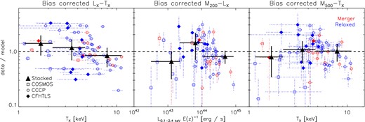
Residuals (defined as the ratio of data to model prediction) for the Eddington bias-corrected LX–TX (left-hand panel), M–LX (middle panel) and M–TX relations. Blue and red dotted data shows the residuals for individual merging and relaxed systems, squares indicate systems from COSMOS, circles from CCCP and solid diamonds from CFHTLS. Large triangles show the median and median standard deviation of stacked residuals for three mass bins.
Stacked residuals of the BC relations.
| M200 <2 × 10¹⁴ M⊙ | M200 =2–8 × 10¹⁴ M⊙ | M200 >8 × 10¹⁴ M⊙ | |
|---|---|---|---|
| Stacked | Stacked | Stacked | |
| data/model | data/model | data/model | |
| LX–TX this work | 1.39 ± 0.55 | 1.16 ± 0.47 | 0.84 ± 0.32 |
| LX–TX literature high-mass sample | 1.33 ± 0.53 | 0.73 ± 0.49 | 0.93 ± 0.21 |
| M200–LX this work | 0.65 ± 0.34 | 1.42 ± 0.73 | 0.81 ± 0.22 |
| M200–LX literature high-mass sample | 0.73 ± 0.40 | 1.11 ± 0.45 | 0.93 ± 0.29 |
| M500–TX this work | 0.79 ± 0.45 | 1.07 ± 0.46 | 1.00 ± 0.36 |
| M500–TX literature high-mass sample | 0.89 ± 0.11 | 1.12 ± 0.65 | 0.85 ± 0.22 |
Notes. This work refers to relations combining COSMOS, CFHTLS and CCCP data, literature high-mass sample to relations combining COSMOS and CFHTLS data corrected to match Chandra calibration with the literature high-mass sample.
For M–LX and M–TX relations where we perform full bias corrections, we find consistent behaviour using both data sets, whereas there is tension for the LX–TX relation. The M–LX and M–TX residuals show that low-mass systems (M200 < 2 × 10¹⁴ M⊙) tend to be below the best-fitting relation, intermediate mass systems (M200 = 2–8 × 10¹⁴ M⊙) above the mean relation and high-mass systems (M200 > 2 × 10¹⁴ M⊙) above or at the best-fitting relation. This is consistent with a mass-dependent scaling where low-mass objects follow a steeper scaling than high-mass objects, with the effect being stronger for the mass–luminosity relation than for the mass–temperature relation. This implies that galaxy groups are warmer and more luminous for their mass than clusters. We also see a tendency for steepening at low masses in the LX–TX relation using CCCP, whereas the literature high-mass sample would result in opposite behaviour.
The strong indications of a mass dependence in the M–LX and M–TX relations show that there is a need to explore more complicated scaling relation than a single power-law arising from self-similar theory. However, due to the lack of theoretical priors for the functional form and large uncertainties of the data, we do not attempt to model a more complicated scaling. The inferred mass dependence can be attributed to the inclusion of intermediate-mass CFHTLS data and proper accounting for observational biases. Indeed, in Kettula et al. (2013b) we studied the scaling of lensing mass to temperature of COSMOS groups and clusters from 160SD and CCCP (with different M and TX measurements than here), and found a single relation connecting groups and high-mass clusters.
Several previous studies have shown that the scaling relation can deviate from the purely gravitational self-similar prediction and that the deviations become stronger for low-mass systems with masses below a few times 1014 M⊙(see e.g. Giodini et al. 2013, and references therein). However, these studies relied on possibly biased HSE mass estimates and this work gives the first indications of different scaling for groups and clusters using accurate lensing masses.
As shown by Fig. 1 and e.g. Giodini et al. (2010), the AGN contribution to the energetics of the intracluster gas increases with decreasing mass. As baryonic feedback becomes significant for galaxy groups, energy injection to the intracluster gas in galaxy groups can lead to different scaling for low-mass systems, as indicated in recent simulations by Planelles et al. (2014), Le Brun et al. (2014) and Pike et al. (2014).
Energy injection to the intracluster gas in galaxy groups may also contribute to HSE mass bias in groups. Indeed, in Kettula et al. (2013b) we report an HSE mass bias increasing with decreasing mass. This is to be contrasted to the analytical model for non-thermal pressure in galaxy clusters by Shi & Komatsu (2014), who infer an HSE mass bias due to turbulence in the intracluster medium which increases with increasing mass, in line with direct lensing measurements reported in Mahdavi et al. (2013), von der Linden et al. (2014b) and Israel et al. (2015). However, the model of Shi & Komatsu (2014) is contradicted by recent simulations (Miniati 2015 and Miniati, private communication), who shows that the turbulence scales with thermal energy and should thus result in an HSE mass bias which is constant in mass. As the non-thermal contribution from AGN becomes significant at group levels, the Miniati simulations would thus result in an HSE mass bias consistent with Kettula et al. (2013b).
Finally, X-ray line emission on group scales may contribute to a break in the mass-to-luminosity relation. Typically the shape of the X-ray spectra of clusters is determined by the bremsstrahlung continuum, but at group masses line emission due to metallicity becomes significant. This results in an extra emission component on top of the bremsstrahlung responsible for > 50 per cent of the total X-ray emission, making groups more luminous for their mass. This is not accounted for by the self-similar model and is qualitatively consistent with our findings above.
5.4 Effects of substructure and triaxiality
Simulations by e.g. Meneghetti et al. (2010) and Becker & Kravtsov (2011) indicate that weak lensing masses obtained by fitting an NFW profiles to tangential shear profiles suffer from a scatter of ∼20–25 per cent (see also discussion in Sereno & Ettori 2014). The main source for the scatter and bias are triaxiality and cluster substructure. Triaxiality and substructure may also bias the resulting masses low by ∼5 per cent. As merging clusters per definition display on average stronger deviations from spherical symmetry than relaxed clusters, we expect them to be more strongly affected by scatter and possible bias related to triaxiality and substructure. The large size of the sample allows us to construct subsamples of relaxed and merging clusters to study this effect. We fit relations to the relaxed and merging subsample, and describe them in Figs 7–9, 10–12 and 13–15, and Table 2.
In the case of the bias-corrected M–LX and M–TX relations, which are affected by biases and scatter in lensing masses, we see a trend for a larger scatter in the merging subsample, albeit at a low statistical significance. We do not find any significant differences in the parameters (see Figs 11 and 14), but note that the relaxed subsample seems to favour steeper slopes than the merging subsample. This could be evidence for some residual bias originating from the cool core (see Section 2.2). We also note that possible biases in the slopes do not affect the scatters (Vikhlinin et al. 2009).
For the LX–TX relation, which is unaffected by lensing masses, we see the opposite trend in scatter, i.e. mergers have a lower scatter (see Table. 2). Once again we find no significant difference in the parameters between merging and relaxed clusters (Fig. 8), but note that merging clusters might favour a steeper slope and higher normalization. This is supported by Bharadwaj et al. (2015), who find a steeper slope and higher normalization for the LX–TX relation of preferentially relaxed strong cool core groups. However, as Bharadwaj et al. (2015) used non-core-excised bolometric luminosities, their trend is most likely driven by the inclusion of bright cool cores.
We test how strongly the above effects are related to uncertainties arising from assuming an NFW profile by comparing the mass residuals of the M–TX relation using 11 merging CCCP clusters with mass measurements determined with the NFW assumption and aperture densitometry, available from Hoekstra et al. (2015). Aperture mass relates shear directly to projected density contrast, without any assumptions of geometry. A change in bias would move the residuals systematically to one direction, whereas scatter is determined from the spread of the distribution. We find no difference in scatter or bias using the two mass measurement methods (see Fig. 20).
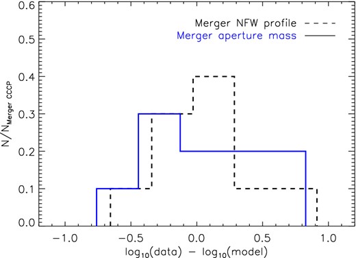
The mass residuals in the mass–temperature relation for merging CCCP clusters. We show the residuals of M500 for all merging CCCP clusters measured using an NFW density profile (dashed black line) and aperture mass (blue solid line) to the best-fitting M–TX relation fitted to all merging clusters in the total sample.
Overall, mergers contribute little to the total scatter for X-ray selected samples such as ours. Our measurements also demonstrate that the intrinsic scatter in temperature at fixed mass is significantly lower than in the luminosity at fixed mass. This shows that temperature is a good low-scatter mass proxy for cluster samples selected on X-ray brightness. However, samples dominated by merging clusters, such as Planck Collaboration XXIX (2013), might have less scatter using other proxies such as gas mass Mgas or thermal energy content of the intracluster gas YX = TX × Mgas. Mahdavi et al. (2013) studied these proxies using the high-mass CCCP sample and found that while Mgas has lower scatter, YX is independent of cluster morphology.
6 SUMMARY AND CONCLUSIONS
We performed weak lensing and X-ray analysis for a sample of 12 individual low-mass clusters within the context of the CFHTLenS and XMM-CFHTLS surveys. This work extends our previous work by inclusion of measurements of intermediate mass systems and provides the first M–LX relation for low-mass systems with individual lensing mass measurements. We find X-ray luminosities between a few times 1043 erg s−1 and a few times 1045 erg s−1, temperatures ranging from ∼2–7 keV and masses M200 of ∼1014–1015 M⊙.
Combining the systems analysed in this work with lower mass COSMOS and higher mass CCCP systems from the literature, we end up with a sample of 70 systems, spanning over two orders of magnitude in mass, three orders of magnitude in luminosity and roughly one order of magnitude in temperature.
We present a correction for Eddington bias and also apply a Malmquist bias correction for the independent variable (x-direction). As our samples are X-ray selected, we are able to provide fully bias-corrected M–LX and M–TX relations. By quoting the relations and intrinsic scatters of the parameters, we provide the current limitations for X-ray luminosity and temperature as cluster mass proxies. We find that the scatter in TX at fixed mass is significantly lower than that of LX. Though observationally more expensive than LX, this feature renders TX an attractive mass proxy for use in cosmological work.
We use the three surveys making up the sample as overlapping mass bins to study mass-dependent effects. As the relations fitted to individual surveys suffer from large statistical uncertainties, we do not find any statistically significant effects. Inspecting residuals for the BC relations, we see for the first time indications that galaxy groups are more luminous and warmer for their mass than clusters using accurate lensing masses, implying a steepening in the scaling relations. We expect this steepening to be stronger for luminosity than for temperature. A steepening implies the need for a more complicated scaling than a single power-law predicted from the purely gravitational self-similar model.
We construct a high-mass sample from the literature to investigate the sensitivity of the relations to the sample. Even after accounting for observational biases and X-ray cross-calibration issues, the literature sample leads to steeper LX–TX and M–TX relations, demonstrating that variance between samples is the dominant effect leading to discrepant scaling. However, the inferred mass dependence of the relations is also present with the literature high-mass sample.
We divide the sample into subsamples of relaxed and merging clusters based on the offset between the X-ray peak and the BCG to investigate the morphology dependence of the scaling. For M–LX and M–TX relations which include lensing masses, we find that mergers may result in enhanced scatter, which we attribute to cluster triaxiality and substructure. For the LX–TX relation which is independent of lensing measurements, we find the opposite trend in scatter. We study if using aperture mass measurements instead of assuming an NFW profile improves the mass measurements for merging systems, but find no significant effect. For the overall relations fitted to the full sample, we find that mergers contribute little. However, for samples dominated by merging systems, lensing mass calibration using other methods than a single NFW profile may lead to improved mass calibration.
We also explore the effects of X-ray cross-calibration and provide scaling relations with our XMM–Newton-based temperatures and luminosities converted to match Chandra calibration. We find that Chandra calibration leads to flatter slopes for LX–TX and M–TX relations, whereas the M–LX relation is unaffected.
In conclusion, our work provides a correction for Eddington bias and fully BC scaling relations over a large mass range. We demonstrate the importance of having well-understood samples on all mass scales and a better understanding of the covariances between selection and observables. We detect the first indications of mass dependent scaling relations using weak lensing masses and demonstrate the need for more observations of low-mass systems in order to accurately measure the inferred mass dependence.
The authors thank the anonymous referee for useful comments and suggestions. This work is based on observations obtained with MegaPrime/MegaCam, a joint project of CFHT and CEA/DAPNIA, at the Canada–France–Hawaii Telescope (CFHT) which is operated by the National Research Council (NRC) of Canada, the Institut National des Sciences de l'Univers of the Centre National de la Recherche Scientifique (CNRS) of France, and the University of Hawaii. This research used the facilities of the Canadian Astronomy Data Centre operated by the National Research Council of Canada with the support of the Canadian Space Agency. CFHTLenS data processing was made possible thanks to significant computing support from the NSERC Research Tools and Instruments grant programme, and to HPC specialist Ovidiu Toader.
KK acknowledges support from Arvid och Greta Ohlins fond and Magnus Ehrnrooth foundation. KK and AF acknowledge Academy of Finland award, decision 1266918. AF, ML and MM have been supported by a DLR project 50 OR 1013 to MPE. CH, HHo, and BR acknowledge support from the European Research Council under the EC FP7 grant numbers 240185 (CH), 279396 (HHo) and 240672 (BR). TDK acknowledges support from a Royal Society University Research Fellowship. TE is supported by the Deutsche Forschungsgemeinschaft through project ER 327/3-1 and is supported by the Transregional Collaborative Research Centre TR 33 – ‘The Dark Universe’. HHi is supported by the Marie Curie IOF 252760, a CITA National Fellowship, and the DFG grant Hi 1495/2-1. HHo, SG acknowledge support from the Netherlands Organisation for Scientific Research grant number 639.042.814. YM acknowledges support from CNRS/INSU (Institut National des Sciences de l'Univers) and the Programme National Galaxies et Cosmologie (PNCG). LVW acknowledges support from the Natural Sciences and Engineering Research Council of Canada (NSERC) and the Canadian Institute for Advanced Research (CIfAR, Cosmology and Gravity program). JPK acknowledge generous support from the ERC advanced grant: LIDA. LF acknowledges support from NSFC grants 11103012 and 11333001 and Shanghai Research grant 13JC1404400. MJH acknowledges support from the Natural Sciences and Engineering Research Council of Canada (NSERC).
Author Contributions: All authors contributed to the development and writing of this paper. The authorship list reflects the lead authors of this paper (KK, SG, EvU, HH, AF, ML) followed by two alphabetical groups. The first alphabetical group includes key contributors to the science analysis and interpretation in this paper, the founding core team and those whose long-term significant effort produced the final CFHTLenS and XMM-CFHTLS data products. The second group covers members of the CFHTLenS and XMM-CFHTLS team who made a significant contribution to the project.
The spherical overdensity radius inside which the density is 500 times the critical density.
Available on http://sfstar.sfsu.edu/cccp/.
REFERENCES
APPENDIX A: COSMOS AND CCCP LUMINOSITIES
The core-excised soft band luminosities for COSMOS are given in Table A1 and for CCCP in Table A2.
The core-excised soft band X-ray luminosities of the COSMOS systems.
| COSMOS | LX |
|---|---|
| xid | 1043 erg s−1 |
| 11 | 3.24 ± 0.11 |
| 17 | 1.81 ± 0.21 |
| 25 | 0.36 ± 0.02 |
| 29 | 1.14 ± 0.14 |
| 120 | 12.02 ± 1.27 |
| 149 | 0.72 ± 0.03 |
| 193 | 0.61 ± 0.05 |
| 220 | 14.38 ± 0.93 |
| 237 | 1.93 ± 0.18 |
| 262 | 2.42 ± 0.25 |
| COSMOS | LX |
|---|---|
| xid | 1043 erg s−1 |
| 11 | 3.24 ± 0.11 |
| 17 | 1.81 ± 0.21 |
| 25 | 0.36 ± 0.02 |
| 29 | 1.14 ± 0.14 |
| 120 | 12.02 ± 1.27 |
| 149 | 0.72 ± 0.03 |
| 193 | 0.61 ± 0.05 |
| 220 | 14.38 ± 0.93 |
| 237 | 1.93 ± 0.18 |
| 262 | 2.42 ± 0.25 |
The core-excised soft band X-ray luminosities of the CCCP systems.
| Cluster | LX |
|---|---|
| name | 1043 erg s−1 |
| 3C295 | 19.24 ± 0.79 |
| Abell0068 | 43.66 ± 1.63 |
| Abell0115N | 35.35 ± 0.70 |
| Abell0115S | 47.58 ± 1.52 |
| Abell0209 | 55.94 ± 0.81 |
| Abell0222 | 22.49 ± 1.16 |
| Abell0223S | 19.90 ± 0.69 |
| Abell0267 | 30.85 ± 0.81 |
| Abell0370 | 40.13 ± 1.39 |
| Abell0383 | 21.17 ± 1.60 |
| Abell0520 | 56.26 ± 1.22 |
| Abell0521 | 53.48 ± 1.20 |
| Abell0586 | 26.57 ± 1.16 |
| Abell0611 | 30.51 ± 0.95 |
| Abell0697 | 76.88 ± 1.80 |
| Abell0851 | 36.15 ± 1.034 |
| Abell0959 | 21.45 ± 1.72 |
| Abell0963 | 43.14 ± 1.13 |
| Abell1689 | 64.57 ± 0.45 |
| Abell1763 | 60.15 ± 1.42 |
| Abell1835 | 68.57 ± 0.52 |
| Abell1914 | 64.83 ± 0.91 |
| Abell1942 | 14.57 ± 0.70 |
| Abell2104 | 66.88 ± 2.11 |
| Abell2111 | 33.98 ± 2.50 |
| Abell2163 | 159.92 ± 2.55 |
| Abell2204 | 57.07 ± 0.42 |
| Abell2218 | 37.63 ± 0.46 |
| Abell2219 | 170.81 ± 1.66 |
| Abell2259 | 24.87 ± 1.17 |
| Abell2261 | 58.15 ± 3.22 |
| Abell2390 | 118.57 ± 1.73 |
| Abell2537 | 32.93 ± 1.23 |
| CL0024.0+1652 | 8.87 ± 1.30 |
| MACSJ0717.5+3745 | 137.73 ± 2.31 |
| MACSJ0913.7+4056 | 26.79 ± 0.69 |
| MS0015.9+1609 | 83.46 ± 2.10 |
| MS0440.5+0204 | 9.15 ± 1.44 |
| MS0451.6-0305 | 86.60 ± 2.66 |
| MS0906.5+1110 | 28.08 ± 0.97 |
| MS1008.1-1224 | 24.74 ± 1.22 |
| MS1231.3+1542 | 14.30 ± 0.49 |
| MS1358.1+6245 | 27.67 ± 1.60 |
| MS1455.0+2232 | 30.35 ± 0.90 |
| MS1512.4+3647 | 12.10 ± 1.10 |
| MS1621.5+2640 | 27.71 ± 1.27 |
| RXJ1347.5-1145 | 131.61 ± 2.01 |
| RXJ1524.6+0957 | 16.93 ± 2.03 |
APPENDIX B: EDDINGTON BIAS CORRECTIONS
The Eddington bias corrections for CFHTLS, COSMOS and CCCP systems are given in Tables B1, B2 and B3, respectively.
The Eddington bias corrections for CFHTLS systems.
| xid | |$\frac{{\rm d} \alpha (ln(M)}{{\rm d} \ln (M)}$| | Mrat | TX, rat | LX, rat |
|---|---|---|---|---|
| 110090 | 0.988 | 0.915 | 0.939 | 0.763 |
| 110460 | 2.265 | 0.816 | 0.703 | 0.538 |
| 110850 | 1.410 | 0.881 | 0.887 | 0.681 |
| 110860 | 0.925 | 0.920 | 0.920 | 0.776 |
| 111180 | 2.220 | 0.819 | 0.903 | 0.547 |
| 210010 | 2.019 | 0.834 | 0.910 | 0.577 |
| 210020 | 0.576 | 0.949 | 0.968 | 0.854 |
| 210630 | 1.334 | 0.887 | 0.792 | 0.694 |
| 210740 | 1.792 | 0.851 | 0.830 | 0.613 |
| 210910 | 2.610 | 0.791 | 0.619 | 0.490 |
| 210970 | 3.042 | 0.761 | 0.824 | 0.437 |
| 102760 | 2.247 | 0.817 | 0.385 | 0.542 |
|$\frac{{\rm d} \alpha (ln(M)}{{\rm d} \ln (M)}$| is the slope of the mass function, Mrat, TX, rat and LX, rat are the ratio of the Eddington BC mass, temperature and luminosity to the uncorrected values.
The Eddington bias corrections for COSMOS systems.
| xid | |$\frac{{\rm d} \alpha (ln(M)}{{\rm d} \ln (M)}$| | Mrat | TX, rat | LX, rat |
|---|---|---|---|---|
| 11 | 0.806 | 0.930 | 0.967 | 0.803 |
| 17 | 0.797 | 0.931 | 0.966 | 0.800 |
| 25 | 0.235 | 0.979 | 0.990 | 0.937 |
| 29 | 0.857 | 0.926 | 0.898 | 0.787 |
| 120 | 0.959 | 0.917 | 0.954 | 0.766 |
| 149 | 0.699 | 0.939 | 0.972 | 0.826 |
| 193 | 0.436 | 0.961 | 0.979 | 0.8863 |
| 220 | 2.274 | 0.815 | 0.884 | 0.536 |
| 237 | 0.538 | 0.952 | 0.914 | 0.861 |
| 262 | 0.526 | 0.953 | 0.877 | 0.864 |
|$\frac{{\rm d} \alpha (ln(M)}{{\rm d} \ln (M)}$| is the slope of the mass function, Mrat, TX, rat and LX, rat are the ratio of the Eddington BC mass, temperature and luminosity to the uncorrected values.
The Eddington bias corrections for CCCP systems.
| Name | |$\frac{{\rm d} \alpha (ln(M)}{{\rm d} \ln (M)}$| | Mrat | TX, rat | LX, rat |
|---|---|---|---|---|
| 3C295 | 2.7246 | 0.783 | 0.890 | 0.476 |
| A68 | 2.3183 | 0.812 | 0.910 | 0.532 |
| A115N | 1.4342 | 0.879 | 0.945 | 0.677 |
| A115S | 1.5806 | 0.868 | 0.939 | 0.651 |
| A209 | 1.7475 | 0.855 | 0.933 | 0.622 |
| A222 | 1.5154 | 0.873 | 0.939 | 0.661 |
| A223S | 1.6967 | 0.859 | 0.930 | 0.630 |
| A267 | 1.719 | 0.857 | 0.932 | 0.627 |
| A370 | 4.2331 | 0.684 | 0.827 | 0.316 |
| A383 | 1.3782 | 0.884 | 0.947 | 0.685 |
| A520 | 2.423 | 0.805 | 0.910 | 0.518 |
| A521 | 2.1272 | 0.826 | 0.920 | 0.561 |
| A586 | 1.2077 | 0.897 | 0.947 | 0.720 |
| A611 | 1.977 | 0.838 | 0.913 | 0.584 |
| A697 | 2.5279 | 0.797 | 0.900 | 0.503 |
| A851 | 3.5767 | 0.726 | 0.864 | 0.378 |
| A959 | 3.0663 | 0.760 | 0.843 | 0.431 |
| A963 | 2.1625 | 0.824 | 0.919 | 0.556 |
| A1689 | 3.5814 | 0.725 | 0.871 | 0.378 |
| A1763 | 2.6444 | 0.789 | 0.901 | 0.487 |
| A1835 | 2.9783 | 0.766 | 0.888 | 0.445 |
| A1914 | 2.2112 | 0.820 | 0.918 | 0.549 |
| A1942 | 2.3255 | 0.812 | 0.910 | 0.530 |
| A2104 | 2.3853 | 0.808 | 0.909 | 0.523 |
| A2111 | 1.8756 | 0.845 | 0.917 | 0.598 |
| A2163 | 2.6381 | 0.789 | 0.904 | 0.488 |
| A2204 | 2.7131 | 0.784 | 0.899 | 0.479 |
| A2218 | 2.4756 | 0.801 | 0.907 | 0.511 |
| A2219 | 2.0995 | 0.829 | 0.921 | 0.566 |
| A2259 | 1.6281 | 0.864 | 0.930 | 0.642 |
| A2261 | 3.2946 | 0.744 | 0.871 | 0.407 |
| A2390 | 3.1878 | 0.752 | 0.884 | 0.421 |
| A2537 | 3.1944 | 0.751 | 0.823 | 0.419 |
| CL0024 | 3.8042 | 0.711 | 0.367 | 0.341 |
| MACS0717 | 5.6275 | 0.604 | 0.798 | 0.217 |
| CL0910 | 1.8656 | 0.846 | 0.924 | 0.602 |
| MS0016 | 4.8253 | 0.649 | 0.801 | 0.269 |
| MS0440 | 1.0189 | 0.913 | 0.940 | 0.749 |
| MS0451 | 3.6064 | 0.724 | 0.855 | 0.375 |
| MS0906 | 2.1382 | 0.826 | 0.917 | 0.559 |
| MS1008 | 2.7792 | 0.780 | 0.885 | 0.469 |
| MS1231 | 0.78512 | 0.932 | 0.968 | 0.808 |
| MS1358 | 2.5624 | 0.795 | 0.876 | 0.497 |
| MS1455 | 2.355 | 0.810 | 0.912 | 0.527 |
| MS1512 | 1.3264 | 0.888 | 0.936 | 0.694 |
| MS1621 | 3.4511 | 0.734 | 0.849 | 0.390 |
| RXJ1347 | 3.5424 | 0.728 | 0.870 | 0.382 |
| RXJ1524 | 2.0217 | 0.834 | 0.890 | 0.569 |
|$\frac{{\rm d} \alpha (ln(M)}{{\rm d} \ln (M)}$| is the slope of the mass function, Mrat, TX, rat and LX, rat are the ratio of the Eddington BC mass, temperature and luminosity to the uncorrected values.
APPENDIX C: LITERATURE HIGH-MASS SAMPLE
We give the X-ray luminosity and temperature measurements and lensing masses of the literature high-mass sample in Table C1. The Eddington bias corrections are described in Table C2.
| Cluster | z | LX | TX | kT | M500 | M200 | Author |
|---|---|---|---|---|---|---|---|
| name | 1043 erg s−1 | keV | ref. | 1014 M⊙ | 1014 M⊙ | code | |
| Abell2029 | 0.0779 | 41.4 ± 3.9 | 8.22 ± 0.16 | 2 | 6.501 ± 1.189 | 10.278 ± 1.88 | cypriano+04 |
| Abell478 | 0.0881 | 48.8 ± 4.7 | 7.96 ± 0.27 | 2 | 9.168 ± 2.452 | 13.857 ± 3.707 | okabe+14b |
| Abell2142 | 0.0904 | 64.3 ± 3.5 | 10.04 ± 0.26 | 2 | 8.777 ± 1.476 | 12.457 ± 2.095 | umetsu+09 |
| Abell2244 | 0.0989 | 27.2 ± 2.7 | 5.37 ± 0.12 | 2 | 3.157 ± 2.391 | 4.678 ± 3.543 | kubo+09 |
| Abell2034 | 0.113 | 28.8 ± 2.7 | 7.15 ± 0.32 | 1 | 5.169 ± 3.1 | 8.086 ± 4.849 | okabe&08 |
| Abell2204 | 0.1511 | 53 ± 5.2 | 8.55 ± 0.58 | 2 | 16.051 ± 2.963 | 23.197 ± 4.283 | applegate+14 |
| Abell2218 | 0.171 | 33.5 ± 3.2 | 6.97 ± 0.37 | 1 | 5.108 ± 1.358 | 7.697 ± 2.047 | mahdavi+13 |
| Abell1914 | 0.1712 | 54.4 ± 5.5 | 9.48 ± 0.49 | 1 | 5.6 ± 1.009 | 8.451 ± 1.523 | mahdavi+13 |
| Abell665 | 0.1818 | 56.5 ± 5.2 | 8.03 ± 0.24 | 1 | 8.186 ± 4.621 | 12.461 ± 7.035 | pedersen&07 |
| Abell520 | 0.203 | 64.1 ± 2 | 7.23 ± 0.23 | 3 | 5.516 ± 1.272 | 8.343 ± 1.925 | mahdavi+13 |
| Abell963 | 0.206 | 34.7 ± 1.5 | 6.08 ± 0.3 | 3 | 4.583 ± 1.637 | 6.623 ± 2.365 | applegate+14 |
| Abell1423 | 0.213 | 39.7 ± 2.4 | 5.75 ± 0.59 | 3 | 11.568 ± 5.823 | 16.282 ± 8.196 | dahle06 |
| Abell773 | 0.217 | 47.7 ± 1.5 | 7.37 ± 0.45 | 3 | 16.757 ± 7.814 | 25.985 ± 12.118 | pedersen&07 |
| Abell2261 | 0.224 | 56.3 ± 2.3 | 6.1 ± 0.32 | 3 | 14.663 ± 2.394 | 21.246 ± 4.09 | umetsu+14 |
| Abell1682 | 0.226 | 49.6 ± 6.1 | 7.01 ± 2.14 | 3 | 4.014 ± 2.307 | 6.048 ± 3.476 | pedersen&07 |
| Abell1763 | 0.2279 | 72.9 ± 3.9 | 6.32 ± 0.4 | 3 | 9.989 ± 2.516 | 15.329 ± 3.86 | mahdavi+13 |
| Abell2219 | 0.2281 | 95.8 ± 5.3 | 10.9 ± 0.53 | 3 | 11.729 ± 1.852 | 16.951 ± 2.677 | applegate+14 |
| Abell2111 | 0.229 | 36.1 ± 2.2 | 6.51 ± 0.72 | 3 | 4.498 ± 1.491 | 6.795 ± 2.251 | mahdavi+13 |
| Abell267 | 0.23 | 33.6 ± 1.6 | 7.13 ± 0.71 | 3 | 5.245 ± 1.523 | 7.948 ± 2.308 | mahdavi+13 |
| Abell2390 | 0.2329 | 86.9 ± 2.9 | 10.28 ± 0.38 | 3 | 11.183 ± 2.396 | 16.162 ± 3.463 | applegate+14 |
| Abell1835 | 0.2528 | 67.3 ± 2.3 | 9.0 ± 0.25 | 3 | 15.51 ± 4.503 | 22.417 ± 6.508 | applegate+14 |
| Abell68 | 0.2546 | 44.2 ± 2.7 | 7.56 ± 0.97 | 3 | 9.171 ± 1.587 | 13.254 ± 2.294 | applegate+14 |
| Abell697 | 0.282 | 89.5 ± 5 | 10.93 ± 1.11 | 3 | 9.531 ± 1.303 | 14.694 ± 2.009 | mahdavi+13 |
| Abell781 | 0.2984 | 51 ± 3.2 | 7.55 ± 1.03 | 3 | 9.655 ± 4.393 | 13.78 ± 6.27 | dahle06 |
| Abell85 | 0.0557 | 30.4 ± 2 | 6.45 ± 0.1 | 2 | 4.579 ± 1.245 | 7.24 ± 1.968 | cypriano+04 |
| Abell2597 | 0.0852 | 12.9 ± 1.3 | 3.58 ± 0.07 | 1 | 2.803 ± 1.047 | 4.432 ± 1.656 | cypriano+04 |
| Abell1689 | 0.1832 | 57.2 ± 5.7 | 9.15 ± 0.35 | 1 | 12.614 ± 1.671 | 16.843 ± 2.429 | umetsu+11 |
| Abell209 | 0.206 | 58 ± 2.2 | 8.23 ± 0.66 | 3 | 11.573 ± 1.796 | 17.559 ± 2.993 | umetsu+14 |
| Abell521 | 0.2475 | 58 ± 2.1 | 6.21 ± 0.28 | 3 | 8.082 ± 1.94 | 11.68 ± 2.803 | applegate+14 |
| Abell2537 | 0.2966 | 38.7 ± 2.9 | 7.63 ± 0.86 | 3 | 7.068 ± 1.113 | 10.841 ± 1.707 | mahdavi+13 |
| MACSJ1115.8+0129 | 0.355 | 54.3 ± 2.5 | 9.2 ± 0.98 | 3 | 9.259 ± 1.991 | 15.531 ± 3.385 | umetsu+14 |
| MACSJ0949.8+1708 | 0.384 | 62.3 ± 4.1 | 8.92 ± 1.83 | 3 | 8.874 ± 4.075 | 12.825 ± 5.889 | applegate+14 |
| MACSJ1731.6+2252 | 0.389 | 74.2 ± 4.3 | 5.87 ± 0.61 | 3 | 22.817 ± 4.087 | 32.977 ± 5.906 | applegate+14 |
| MACSJ2211.7-0349 | 0.396 | 101.5 ± 6.3 | 13.97 ± 2.74 | 3 | 13.447 ± 2.881 | 19.434 ± 4.164 | applegate+14 |
| MACSJ0429.6-0253 | 0.399 | 39.1 ± 2.5 | 8.33 ± 1.58 | 3 | 6.765 ± 1.89 | 9.351 ± 2.984 | umetsu+14 |
| MACSJ1206.2-0847 | 0.439 | 105.5 ± 6.4 | 10.71 ± 1.29 | 3 | 10.542 ± 2.089 | 15.813 ± 3.58 | umetsu+14 |
| MACSJ0417.5-1154 | 0.443 | 152.9 ± 9.4 | 9.49 ± 1.12 | 3 | 21.176 ± 3.97 | 30.605 ± 5.738 | applegate+14 |
| MACSJ2243.3-0935 | 0.447 | 115.6 ± 6.7 | 8.24 ± 0.92 | 3 | 20.294 ± 3.865 | 29.33 ± 5.587 | applegate+14 |
| RXJ0439.0+0715 | 0.2443 | 42.2 ± 1.6 | 6.59 ± 0.45 | 3 | 9.753 ± 4.955 | 13.792 ± 7.006 | dahle06 |
| Zwicky5247 | 0.229 | 37.4 ± 2.4 | 5.31 ± 1.07 | 3 | 2.472 ± 2.042 | 3.49 ± 2.883 | dahle06 |
| Zwicky2089 | 0.2347 | 17 ± 1.3 | 6.55 ± 1.47 | 3 | 3.55 ± 2.965 | 5.02 ± 4.193 | dahle06 |
| Zwicky3146 | 0.2906 | 58.2 ± 2.6 | 8.38 ± 0.44 | 3 | 12.071 ± 5.271 | 18.72 ± 8.175 | pedersen&07 |
z, LX and TX are redshift, core-excised X-ray temperature and core-excised soft band luminosity of the cluster from Mantz et al. (2010). kT ref. gives the reference for temperatures in Mantz et al. (2010), (1) are ASCA temperatures from Horner (2001), 2 and 3 are Chandra temperatures from Vikhlinin et al. (2009) and Mantz et al. (2010). M500, M200 and author code the spherical overdensity masses with respect to the critical density and author code fields in the LC2 catalogue of Sereno (2014). Author code applegate+14 points to Applegate et al. (2014), cypriano+04 to Cypriano et al. (2004), dahle06 to Dahle (2006), kubo+09 to Kubo et al. (2009), mahdavi+13 to Mahdavi et al. (2013), okabe&08 to Okabe & Umetsu (2008), okabe+14b to Okabe et al. (2014), pedersen&07 to Pedersen & Dahle (2007), umetsu+09 to Umetsu et al. (2009), umetsu+11 to Umetsu et al. (2011) and umetsu+14 to Umetsu et al. (2014).
| Cluster | z | LX | TX | kT | M500 | M200 | Author |
|---|---|---|---|---|---|---|---|
| name | 1043 erg s−1 | keV | ref. | 1014 M⊙ | 1014 M⊙ | code | |
| Abell2029 | 0.0779 | 41.4 ± 3.9 | 8.22 ± 0.16 | 2 | 6.501 ± 1.189 | 10.278 ± 1.88 | cypriano+04 |
| Abell478 | 0.0881 | 48.8 ± 4.7 | 7.96 ± 0.27 | 2 | 9.168 ± 2.452 | 13.857 ± 3.707 | okabe+14b |
| Abell2142 | 0.0904 | 64.3 ± 3.5 | 10.04 ± 0.26 | 2 | 8.777 ± 1.476 | 12.457 ± 2.095 | umetsu+09 |
| Abell2244 | 0.0989 | 27.2 ± 2.7 | 5.37 ± 0.12 | 2 | 3.157 ± 2.391 | 4.678 ± 3.543 | kubo+09 |
| Abell2034 | 0.113 | 28.8 ± 2.7 | 7.15 ± 0.32 | 1 | 5.169 ± 3.1 | 8.086 ± 4.849 | okabe&08 |
| Abell2204 | 0.1511 | 53 ± 5.2 | 8.55 ± 0.58 | 2 | 16.051 ± 2.963 | 23.197 ± 4.283 | applegate+14 |
| Abell2218 | 0.171 | 33.5 ± 3.2 | 6.97 ± 0.37 | 1 | 5.108 ± 1.358 | 7.697 ± 2.047 | mahdavi+13 |
| Abell1914 | 0.1712 | 54.4 ± 5.5 | 9.48 ± 0.49 | 1 | 5.6 ± 1.009 | 8.451 ± 1.523 | mahdavi+13 |
| Abell665 | 0.1818 | 56.5 ± 5.2 | 8.03 ± 0.24 | 1 | 8.186 ± 4.621 | 12.461 ± 7.035 | pedersen&07 |
| Abell520 | 0.203 | 64.1 ± 2 | 7.23 ± 0.23 | 3 | 5.516 ± 1.272 | 8.343 ± 1.925 | mahdavi+13 |
| Abell963 | 0.206 | 34.7 ± 1.5 | 6.08 ± 0.3 | 3 | 4.583 ± 1.637 | 6.623 ± 2.365 | applegate+14 |
| Abell1423 | 0.213 | 39.7 ± 2.4 | 5.75 ± 0.59 | 3 | 11.568 ± 5.823 | 16.282 ± 8.196 | dahle06 |
| Abell773 | 0.217 | 47.7 ± 1.5 | 7.37 ± 0.45 | 3 | 16.757 ± 7.814 | 25.985 ± 12.118 | pedersen&07 |
| Abell2261 | 0.224 | 56.3 ± 2.3 | 6.1 ± 0.32 | 3 | 14.663 ± 2.394 | 21.246 ± 4.09 | umetsu+14 |
| Abell1682 | 0.226 | 49.6 ± 6.1 | 7.01 ± 2.14 | 3 | 4.014 ± 2.307 | 6.048 ± 3.476 | pedersen&07 |
| Abell1763 | 0.2279 | 72.9 ± 3.9 | 6.32 ± 0.4 | 3 | 9.989 ± 2.516 | 15.329 ± 3.86 | mahdavi+13 |
| Abell2219 | 0.2281 | 95.8 ± 5.3 | 10.9 ± 0.53 | 3 | 11.729 ± 1.852 | 16.951 ± 2.677 | applegate+14 |
| Abell2111 | 0.229 | 36.1 ± 2.2 | 6.51 ± 0.72 | 3 | 4.498 ± 1.491 | 6.795 ± 2.251 | mahdavi+13 |
| Abell267 | 0.23 | 33.6 ± 1.6 | 7.13 ± 0.71 | 3 | 5.245 ± 1.523 | 7.948 ± 2.308 | mahdavi+13 |
| Abell2390 | 0.2329 | 86.9 ± 2.9 | 10.28 ± 0.38 | 3 | 11.183 ± 2.396 | 16.162 ± 3.463 | applegate+14 |
| Abell1835 | 0.2528 | 67.3 ± 2.3 | 9.0 ± 0.25 | 3 | 15.51 ± 4.503 | 22.417 ± 6.508 | applegate+14 |
| Abell68 | 0.2546 | 44.2 ± 2.7 | 7.56 ± 0.97 | 3 | 9.171 ± 1.587 | 13.254 ± 2.294 | applegate+14 |
| Abell697 | 0.282 | 89.5 ± 5 | 10.93 ± 1.11 | 3 | 9.531 ± 1.303 | 14.694 ± 2.009 | mahdavi+13 |
| Abell781 | 0.2984 | 51 ± 3.2 | 7.55 ± 1.03 | 3 | 9.655 ± 4.393 | 13.78 ± 6.27 | dahle06 |
| Abell85 | 0.0557 | 30.4 ± 2 | 6.45 ± 0.1 | 2 | 4.579 ± 1.245 | 7.24 ± 1.968 | cypriano+04 |
| Abell2597 | 0.0852 | 12.9 ± 1.3 | 3.58 ± 0.07 | 1 | 2.803 ± 1.047 | 4.432 ± 1.656 | cypriano+04 |
| Abell1689 | 0.1832 | 57.2 ± 5.7 | 9.15 ± 0.35 | 1 | 12.614 ± 1.671 | 16.843 ± 2.429 | umetsu+11 |
| Abell209 | 0.206 | 58 ± 2.2 | 8.23 ± 0.66 | 3 | 11.573 ± 1.796 | 17.559 ± 2.993 | umetsu+14 |
| Abell521 | 0.2475 | 58 ± 2.1 | 6.21 ± 0.28 | 3 | 8.082 ± 1.94 | 11.68 ± 2.803 | applegate+14 |
| Abell2537 | 0.2966 | 38.7 ± 2.9 | 7.63 ± 0.86 | 3 | 7.068 ± 1.113 | 10.841 ± 1.707 | mahdavi+13 |
| MACSJ1115.8+0129 | 0.355 | 54.3 ± 2.5 | 9.2 ± 0.98 | 3 | 9.259 ± 1.991 | 15.531 ± 3.385 | umetsu+14 |
| MACSJ0949.8+1708 | 0.384 | 62.3 ± 4.1 | 8.92 ± 1.83 | 3 | 8.874 ± 4.075 | 12.825 ± 5.889 | applegate+14 |
| MACSJ1731.6+2252 | 0.389 | 74.2 ± 4.3 | 5.87 ± 0.61 | 3 | 22.817 ± 4.087 | 32.977 ± 5.906 | applegate+14 |
| MACSJ2211.7-0349 | 0.396 | 101.5 ± 6.3 | 13.97 ± 2.74 | 3 | 13.447 ± 2.881 | 19.434 ± 4.164 | applegate+14 |
| MACSJ0429.6-0253 | 0.399 | 39.1 ± 2.5 | 8.33 ± 1.58 | 3 | 6.765 ± 1.89 | 9.351 ± 2.984 | umetsu+14 |
| MACSJ1206.2-0847 | 0.439 | 105.5 ± 6.4 | 10.71 ± 1.29 | 3 | 10.542 ± 2.089 | 15.813 ± 3.58 | umetsu+14 |
| MACSJ0417.5-1154 | 0.443 | 152.9 ± 9.4 | 9.49 ± 1.12 | 3 | 21.176 ± 3.97 | 30.605 ± 5.738 | applegate+14 |
| MACSJ2243.3-0935 | 0.447 | 115.6 ± 6.7 | 8.24 ± 0.92 | 3 | 20.294 ± 3.865 | 29.33 ± 5.587 | applegate+14 |
| RXJ0439.0+0715 | 0.2443 | 42.2 ± 1.6 | 6.59 ± 0.45 | 3 | 9.753 ± 4.955 | 13.792 ± 7.006 | dahle06 |
| Zwicky5247 | 0.229 | 37.4 ± 2.4 | 5.31 ± 1.07 | 3 | 2.472 ± 2.042 | 3.49 ± 2.883 | dahle06 |
| Zwicky2089 | 0.2347 | 17 ± 1.3 | 6.55 ± 1.47 | 3 | 3.55 ± 2.965 | 5.02 ± 4.193 | dahle06 |
| Zwicky3146 | 0.2906 | 58.2 ± 2.6 | 8.38 ± 0.44 | 3 | 12.071 ± 5.271 | 18.72 ± 8.175 | pedersen&07 |
z, LX and TX are redshift, core-excised X-ray temperature and core-excised soft band luminosity of the cluster from Mantz et al. (2010). kT ref. gives the reference for temperatures in Mantz et al. (2010), (1) are ASCA temperatures from Horner (2001), 2 and 3 are Chandra temperatures from Vikhlinin et al. (2009) and Mantz et al. (2010). M500, M200 and author code the spherical overdensity masses with respect to the critical density and author code fields in the LC2 catalogue of Sereno (2014). Author code applegate+14 points to Applegate et al. (2014), cypriano+04 to Cypriano et al. (2004), dahle06 to Dahle (2006), kubo+09 to Kubo et al. (2009), mahdavi+13 to Mahdavi et al. (2013), okabe&08 to Okabe & Umetsu (2008), okabe+14b to Okabe et al. (2014), pedersen&07 to Pedersen & Dahle (2007), umetsu+09 to Umetsu et al. (2009), umetsu+11 to Umetsu et al. (2011) and umetsu+14 to Umetsu et al. (2014).
The Eddington bias corrections for the literature high-mass sample.
| Name | |$\frac{{\rm d} \alpha (ln(M)}{{\rm d} \ln (M)}$| | Mrat | TX, rat | LX, rat |
|---|---|---|---|---|
| Abell2029 | 1.879 | 0.845 | 0.930 | 0.595 |
| Abell478 | 2.244 | 0.817 | 0.916 | 0.538 |
| Abell2142 | 2.116 | 0.827 | 0.921 | 0.561 |
| Abell2244 | 1.234 | 0.895 | 0.953 | 0.710 |
| Abell2034 | 1.689 | 0.859 | 0.935 | 0.627 |
| Abell2204 | 3.163 | 0.753 | 0.879 | 0.417 |
| Abell2218 | 1.725 | 0.856 | 0.933 | 0.621 |
| Abell1914 | 1.818 | 0.849 | 0.930 | 0.604 |
| Abell665 | 2.282 | 0.815 | 0.915 | 0.533 |
| Abell520 | 1.854 | 0.846 | 0.930 | 0.603 |
| Abell963 | 1.635 | 0.863 | 0.937 | 0.640 |
| Abell1423 | 2.724 | 0.783 | 0.888 | 0.474 |
| Abell773 | 3.555 | 0.727 | 0.867 | 0.380 |
| Abell2261 | 3.193 | 0.751 | 0.881 | 0.419 |
| Abell1682 | 1.582 | 0.867 | 0.868 | 0.643 |
| Abell1763 | 2.665 | 0.787 | 0.898 | 0.483 |
| Abell2219 | 2.821 | 0.776 | 0.894 | 0.462 |
| Abell2111 | 1.691 | 0.859 | 0.927 | 0.629 |
| Abell267 | 1.847 | 0.847 | 0.923 | 0.604 |
| Abell2390 | 2.757 | 0.781 | 0.898 | 0.472 |
| Abell1835 | 3.369 | 0.739 | 0.878 | 0.399 |
| Abell68 | 2.511 | 0.798 | 0.889 | 0.503 |
| Abell697 | 2.723 | 0.783 | 0.888 | 0.475 |
| Abell781 | 2.663 | 0.787 | 0.880 | 0.482 |
| Abell85 | 1.516 | 0.872 | 0.943 | 0.660 |
| Abell2597 | 1.185 | 0.899 | 0.955 | 0.720 |
| Abell1689 | 2.709 | 0.784 | 0.899 | 0.472 |
| Abell209 | 2.826 | 0.776 | 0.889 | 0.463 |
| Abell521 | 2.325 | 0.811 | 0.912 | 0.531 |
| Abell2537 | 2.325 | 0.811 | 0.901 | 0.528 |
| MACSJ1115.8+0129 | 2.987 | 0.765 | 0.877 | 0.443 |
| MACSJ0949.8+1708 | 2.751 | 0.781 | 0.847 | 0.471 |
| MACSJ1731.6+2252 | 4.651 | 0.659 | 0.816 | 0.280 |
| MACSJ2211.7-0349 | 3.500 | 0.730 | 0.815 | 0.384 |
| MACSJ0429.6-0253 | 2.337 | 0.811 | 0.875 | 0.527 |
| MACSJ1206.2-0847 | 3.236 | 0.748 | 0.863 | 0.412 |
| MACSJ0417.5-1154 | 4.661 | 0.658 | 0.809 | 0.279 |
| MACSJ2243.3-0935 | 4.569 | 0.664 | 0.816 | 0.287 |
| RXJ0439.0+0715 | 2.546 | 0.795 | 0.901 | 0.500 |
| Zwicky5247 | 1.176 | 0.899 | 0.932 | 0.724 |
| Zwicky2089 | 1.439 | 0.879 | 0.911 | 0.673 |
| Zwicky3146 | 3.142 | 0.754 | 0.883 | 0.424 |
|$\frac{{\rm d} \alpha (ln(M)}{{\rm d} \ln (M)}$| is the slope of the mass function, Mrat, TX,rat and LX,rat are the ratio of the Eddington BC mass, temperature and luminosity to the uncorrected values.
