An exploration of galaxy–galaxy lensing and galaxy clustering in the Millennium-XXL simulation

Marian, Laura; Smith, Robert E.; Angulo, Raul E.

doi:10.1093/mnras/stv984

Abstract

The combination of galaxy–galaxy lensing and galaxy clustering data has the potential to simultaneously constrain both the cosmological and galaxy formation models. In this paper, we perform a comprehensive exploration of these signals and their covariances through a combination of analytic and numerical approaches. First, we derive analytic expressions for the projected galaxy correlation function and stacked tangential shear profile and their respective covariances, which include Gaussian and discreteness noise terms. Secondly, we measure these quantities from mock galaxy catalogues obtained from the Millennium-XXL simulation and semi-analytic models of galaxy formation. We find that on large scales (R > 10 h⁻¹ Mpc), the galaxy bias is roughly linear and deterministic. On smaller scales (R ≲ 5 h⁻¹ Mpc), the bias is a complicated function of scale and luminosity, determined by the different spatial distribution and abundance of satellite galaxies present when different magnitude cuts are applied, as well as by the mass dependence of the host haloes on magnitude. Our theoretical model for the covariances provides a reasonably good description of the measured ones on small and large scales. However, on intermediate scales (1 < R < 10 h⁻¹ Mpc), the predicted errors are ∼2–3 times smaller, suggesting that the inclusion of higher order, non-Gaussian terms in the covariance will be required for further improvements. Importantly, both our theoretical and numerical methods show that the galaxy–galaxy lensing and clustering signals have a non-zero cross-covariance matrix with significant bin-to-bin correlations. Future surveys aiming to combine these probes must take this into account in order to obtain unbiased and realistic constraints.

gravitational lensing: weak, galaxies: statistics, cosmology: theory, large-scale structure of Universe

1 INTRODUCTION

Since the first pioneering attempt to measure the galaxy–galaxy lensing (hereafter GGL) signal by Tyson et al. (1984), there have been significant technological developments in deep and wide-field astronomy, which have led to the emergence of GGL as one of the most promising probes for simultaneously constraining both the cosmological and galaxy formation models.

The first robust detection of the GGL signal was made by Brainerd, Blandford & Smail (1996) using 90 arcmin² of imaging data from the 5 m Palomar telescope. They showed that whilst the tangential shear profile around individual galaxies was too weak to be measured, the stacked signal around all lens galaxies could be detected with high signal-to-noise. Since then there has been a rapid explosion in the field: the addition of the Wide-Field Camera to the Hubble Space Telescope enabled a number of key GGL studies (dell'Antonio & Tyson 1996; Griffiths et al. 1996; Hudson et al. 1998; Leauthaud et al. 2012). The improvement of ground-based facilities such as the Canada–France–Hawaii Telescope has also led to significant developments (Wilson et al. 2001; Hoekstra, Yee & Gladders 2004; Parker et al. 2007; van Uitert et al. 2011; Hudson et al. 2015; Velander et al. 2014). However, perhaps the most prolific work in this area comes from the analysis of the data from the Sloan Digital Sky Survey (hereafter SDSS; Guzik & Seljak 2001, 2002; McKay et al. 2001; Hirata et al. 2004; Sheldon et al. 2004, 2009a,b; Mandelbaum et al. 2005, 2006a,b,c, 2013; Johnston et al. 2007; Nakajima et al. 2012). All these works have revealed that the GGL signal is a complex function depending on a number of galaxy properties, such as luminosity, colour, spectral type, etc. The key importance of GGL is that it enables one to make a direct link from galaxy properties to the underlying dark matter distribution. Indeed, these works have also constrained the mass, density profiles, ellipticity of the dark matter haloes hosting the lens galaxies.

One of the first to realize that cosmic shear could help to simultaneously constrain galaxy formation and cosmology, through directly measuring the bias, was Schneider (1998). Schneider's approach of using aperture mass filters was implemented by Hoekstra et al. (2002) who directly measured galaxy bias, establishing that it was a complicated function of scale. This approach was further theoretically developed for the halo occupation distribution framework by Guzik & Seljak (2001) and later by Seljak et al. (2005) and Yoo et al. (2006). More recent work has been performed by Cacciato et al. (2009, 2013) who have combined the results from GGL and galaxy clustering (hereafter GC) studies, along with measurements of the galaxy luminosity function (hereafter GLF) from SDSS to constrain the parameters of the conditional luminosity function (hereafter CLF) model – which fully specifies the link between a given dark matter halo and the galaxies it hosts, albeit with assumptions about the functional form of the CLF (Yang, Mo & van den Bosch 2003; van den Bosch et al. 2013). An interesting result to emerge from this work was that if one did not include the GGL measurements in the analysis, then equally good fits to the CLF model parameters could be obtained for either Wilkinson Microwave Anisotropy Probe 1 (WMAP1) or WMAP3 cosmology (Spergel et al. 2003, 2007). Including the GGL data broke this degeneracy and identified the WMAP3 parameters as the preferred cosmological model. See also the very recent works of Miyatake et al. (2013) and More et al. (2014).

Whilst there has been significant progress in attempting to understand and interpret the GGL signal (see also Baldauf et al. 2010; Saghiha et al. 2012), our understanding of how to perform a robust likelihood analysis with such data sets has been lacking. For example, in the recent development of the CLF framework (Cacciato et al. 2013; More et al. 2013; van den Bosch et al. 2013), the GGL and GLF measurements were taken to have diagonal covariance matrices, and the GC covariance matrix was obtained from jackknife estimation. Moreover, these probes were assumed to have zero cross-covariance. This is clearly a simplification that future large data set analyses should improve on. A better analysis of the errors was performed by Leauthaud et al. (2012) who used numerical simulations to estimate the covariance matrices of the GGL and GC measurements, while Mandelbaum et al. (2013) used the jackknife approach. The very recent works of Miyatake et al. (2013) and More et al. (2014) also had an improved error analysis. However, again in their analyses the cross-covariance of the two measurements was assumed to be negligible.

If upcoming surveys such as Dark Energy Survey (DES), The Javalambre-Physics of the Accelerated Universe Astrophysical Survey (J-PAS), Euclid and Large Synoptic Survey Telescope (LSST) are to optimally constrain the cosmological model, then it is inevitable that they must also jointly constrain the model of galaxy formation. The best way to do this will be to combine the GGL, GC and GLF measurements. This will require not only accurate models for the signals themselves, but also accurate modelling of the covariance and cross-covariance matrices of these probes.

In this paper, we develop an analytical framework to compute both the covariance and cross-covariance of GC and GGL. Our work builds upon the analysis of the earlier work of Jeong, Komatsu & Jain (2009) for GGL and that of Smith & Marian (2014, 2015) for the GC signal. We then use the semi-analytic galaxy catalogues and dark matter distribution from the Millennium-XXL (hereafter MXXL) simulation (Angulo et al. 2012) to directly measure these observables and their associated auto- and cross-covariances, for several bins in luminosity. Unlike the CLF approach, semi-analytic models (hereafter SAM) make no direct assumption on how galaxies populate dark matter haloes. Instead, they attempt to model the relevant physical processes for galaxy formation and evolution, and how these are affected by environment and assembly history. Thus, the non-linearity and stochasticity of galaxy bias are predictions, not assumptions in our study.

The paper is structured as follows. In Section 2, we present the necessary theoretical expressions for modelling the stacked tangential shear profiles and projected GC signals. In Section 3, we present expressions for their associated auto- and cross-covariances. In Section 4, we provide an overview of the MXXL simulation and the SAM galaxy catalogues that we use. In Section 5, we present the measurements of the GGL and GC signals for a set of luminosity bins, and compare them with the predictions from the theory. In Section 6, we present our results for the GC and GGL covariance and cross-covariance matrices. In Section 7, we summarize our findings and draw our conclusions.

2 THEORETICAL PREDICTIONS FOR THE GGL AND GC SIGNALS

In this section, we present theoretical expressions for the stacked tangential shear signal of a population of galaxy lenses and the signal for the projected galaxy correlation function.

2.1 Overview of required lensing ingredients

In the flat-sky approximation, the complex shear is written in terms of the convergence as (Bartelmann & Schneider 2001)

\begin{equation} \gamma ({\boldsymbol \theta})=\frac{1}{\pi }\int _{\boldsymbol {R}^2} \mathrm{d}^2\theta ^{\prime } \kappa ({\boldsymbol \theta}^{\prime })\mathcal {D}({\boldsymbol \theta}-{\boldsymbol \theta}^{\prime })\,, \end{equation}

(1)

where the lensing kernel is defined to be

\begin{equation} \mathcal {D}({\boldsymbol \theta})\equiv \left(\theta _y^2-\theta _x^2- 2 {\rm i} \theta _x \theta _y\right)/|{\boldsymbol \theta}|^4, \end{equation}

(2)

with θ_x and θ_y being the Cartesian components of the Euclidean vector |${\boldsymbol \theta}=(\theta _x,\theta _y)$|⁠. These equations can be written in Fourier space as

\begin{equation} \gamma ({\boldsymbol l})=\frac{1}{\pi }\kappa ({\boldsymbol l}) \mathcal {D}({\boldsymbol l}),\quad {\rm with}\quad\mathcal {D}({\boldsymbol l})=\pi \frac{l_x^2-l_y^2 + 2 {\rm i} l_x l_y}{|{\boldsymbol l}|^2}, \end{equation}

(3)

where l_x and l_y are the Cartesian components of the vector |${\boldsymbol l}$|⁠; |$\gamma ({\boldsymbol l})$| and |$\mathcal {D}({\boldsymbol l})$| and are the Fourier transforms of |$\gamma ({\boldsymbol \theta})$| and |$\mathcal {D}({\boldsymbol \theta})$|⁠, respectively. From equation (3), the complex shear can also be written using the polar coordinates of the Fourier vector |${\boldsymbol l}$| as

\begin{equation} \gamma ({\boldsymbol l})=\gamma _1({\boldsymbol l}) + {\rm i} \gamma _2({\boldsymbol l})=\kappa ({\boldsymbol l})[\cos (2\phi _{{\boldsymbol l}}) + {\rm i} \sin (2\phi _{{\boldsymbol l}})]. \end{equation}

(4)

The tangential shear at position |${\boldsymbol \theta}$| with respect to position |${\boldsymbol \theta}_0$| (where |${\boldsymbol \theta}$| and |${\boldsymbol \theta}_0$| are defined with respect to the same origin) is

\begin{equation} \gamma _t({\boldsymbol \theta}; {\boldsymbol \theta}_0)=-\gamma _1({\boldsymbol \theta})\cos (2\phi _{{\boldsymbol \theta}-{\boldsymbol \theta}_0}) -\gamma _2({\boldsymbol \theta})\sin (2\phi _{{\boldsymbol \theta}-{\boldsymbol \theta}_0}), \end{equation}

(5)

where |$\phi _{{\boldsymbol \theta}-{\boldsymbol \theta}_0}$| is the polar angle of the relative position vector |${\boldsymbol \theta}-{\boldsymbol \theta}_0$|⁠. Combining the last two equations, one can write

\begin{equation} \gamma _t({\boldsymbol \theta}; {\boldsymbol \theta}_0)=-\int \frac{\mathrm{d}^2 l}{(2\pi )^2} \kappa ({\boldsymbol l})\cos [2(\phi _{{\boldsymbol \theta}-{\boldsymbol \theta}_0}-\phi _{{\boldsymbol l}})] \,{\rm e}^{{\rm i}\, {\boldsymbol l}\cdot {\boldsymbol \theta}} \,. \end{equation}

(6)

Finally, we define the azimuthal average of the tangential shear as

\begin{equation} \gamma _{t,a}(\theta ; {\boldsymbol \theta}_0)=\int _0^{2\pi } \frac{\mathrm{d}\phi _{{\boldsymbol \theta}-{\boldsymbol \theta}_0}}{2\pi }\gamma _t({\boldsymbol \theta}; {\boldsymbol \theta}_0). \end{equation}

(7)

With the help of the very useful Bessel relation

\begin{equation} J_{n}(x)=\int _{\alpha }^{2\pi -\alpha } \frac{\mathrm{d}\phi }{2\pi }\, {\rm e}^{{\rm i}\, [n\phi -x\sin (\phi )]} \,, \end{equation}

(8)

one obtains the following equation which will recur many times in this section:

\begin{equation} J_2(x)=-\int _0^{2\pi } \frac{\mathrm{d}\phi }{2\pi }\cos [2(\phi -\phi ^{\prime })]{\rm e}^{{\rm i}\, x \cos (\phi -\phi ^{\prime })}. \end{equation}

(9)

Therefore, the azimuthal average of the tangential shear is

\begin{equation} {\gamma _{t,a}}(\theta ; {\boldsymbol \theta}_0)=\int \frac{\mathrm{d}^2 l}{(2\pi )^2} \kappa ({\boldsymbol l})J_2(l\theta ) {\rm e}^{{\rm i}\,{\boldsymbol l}\cdot {\boldsymbol \theta}_0}. \end{equation}

(10)

2.2 Estimator for the stacked tangential shear

In GGL, the signal of individual lenses is very weak, so in order to improve the signal-to-noise of this probe, one has to stack several lenses. Suppose there is a population of N_g galaxy lenses at positions |${\boldsymbol x}_i$| in a chosen coordinate system. Also suppose the total area of the survey to be ∫d²x = Ω_s. The number density of these lenses can be written as a sum over their positions:

\begin{equation} n_g({\boldsymbol x})=\sum _{i=1}^{N_{g}}\delta _D({\boldsymbol x}-{\boldsymbol x}_i) \,, \end{equation}

(11)

where |${\boldsymbol x}$| is a 2D vector in the survey area. Using the above equation, an estimator for the tangential shear of such a lens population at an arbitrary position |${\boldsymbol \theta}$| with respect to the location of the galaxy centres |${\boldsymbol x}_i$| is (Jeong et al. 2009)

\begin{eqnarray} \widehat{\gamma }_t^g({\boldsymbol \theta}) & = & \frac{1}{N_g}\sum _{i=1}^{N_{g}}\gamma _t({\boldsymbol x}_i+{\boldsymbol \theta}; {\boldsymbol x}_i) {\nonumber }\\ & = & \frac{1}{N_{g}}\int _{\Omega _s}\mathrm{d}^2x\,n_g({\boldsymbol x})\gamma _t({\boldsymbol x}+{\boldsymbol \theta}; {\boldsymbol x}) \,. \end{eqnarray}

(12)

We define the fluctuation in the number density of lenses as |$n_g({\boldsymbol x})=\bar{n}_g[1+\delta _g({\boldsymbol x})]$|⁠, where the mean angular density of lens galaxies is |$\bar{n}_g=N_g/\Omega _s$|⁠. At this point, we also introduce the definitions of the convergence and galaxy density auto- and cross-power spectra, which shall be used throughout this paper:

\begin{eqnarray} \left\langle \kappa ({\boldsymbol l})\kappa ({\boldsymbol l}^{\prime })\right\rangle & = & (2\pi )^2\delta _D({\boldsymbol l}+{\boldsymbol l}^{\prime })\mathcal {C}_{\kappa \kappa }(l); \nonumber \\ \left\langle \delta _g({\boldsymbol l}) \delta _g({\boldsymbol l}^{\prime })\right\rangle & = & (2\pi )^2\delta _D({\boldsymbol l}+{\boldsymbol l}^{\prime })\mathcal {C}_{g g}(l); \nonumber \\ \left\langle \delta _g({\boldsymbol l})\kappa ({\boldsymbol l}^{\prime })\right\rangle & = & (2\pi )^2\delta _D({\boldsymbol l}+{\boldsymbol l}^{\prime })\mathcal {C}_{g\kappa }(l). \end{eqnarray}

(13)

Since the tangential shear with respect to an origin |${\boldsymbol 0}$| vanishes on average |$\langle \gamma _t({\boldsymbol \theta}| {\boldsymbol 0})\rangle =0$|⁠, the ensemble average of the estimator in equation (12) is

\begin{eqnarray} \left\langle \widehat{\gamma }_t^g({\boldsymbol \theta})\right\rangle & = &\frac{1}{N_g} \int _{\Omega _s}\mathrm{d}^2x\,\left\langle n_g({\boldsymbol x})\gamma _t({\boldsymbol x}+{\boldsymbol \theta}; {\boldsymbol x})\right\rangle {\nonumber }\\ & = & \frac{1}{\Omega _s}\int _{\Omega _s}\mathrm{d}^2x\,\left\langle \delta _g({\boldsymbol x})\gamma _t({\boldsymbol x}+{\boldsymbol \theta}; {\boldsymbol x})\right\rangle {\nonumber }\\ & = & \left\langle \delta _g({\bf 0})\gamma _t({\boldsymbol \theta}; {\bf 0})\right\rangle {\nonumber }\\ & = & -\int \frac{\mathrm{d}^2l}{(2\pi )^2}\mathcal {C}_{g\kappa }(l) \cos [2(\phi _{{\boldsymbol \theta}}-\phi _{{\boldsymbol l}})]{\rm e}^{{\rm i} \,{\boldsymbol l}\cdot {\boldsymbol \theta}}. \end{eqnarray}

(14)

In the above we have also used the homogeneity of the Universe, which makes the ensemble average of two cosmological fields to be invariant under translations. We shall take advantage extensively of this property throughout this work. With equation (9), we arrive at the azimuthally-averaged expression for the ensemble average of the stacked shear estimator:

\begin{equation} \left\langle \widehat{\gamma }_{t,a}^g(\theta )\right\rangle = \int \frac{\mathrm{d}^2l}{(2\pi )^2}\mathcal {C}_{g\kappa }(l)J_2(l \theta ). \end{equation}

(15)

Our goal is to compare theory predictions with estimates from simulations, so we must take into account that the measured tangential shear is bin averaged and not just azimuthally averaged. We introduce the bin area:

\begin{equation} A(\theta _i)\equiv \int _0^{2\pi } \mathrm{d}\phi _{\boldsymbol \theta}\int _{\theta _{\rm min}^i}^{\theta ^i_{\max}} \mathrm{d}\theta \,\theta =\pi \left(\theta ^{i\,2}_{\max}-\theta ^{i\,2}_{\rm min}\right), \end{equation}

(16)

with |$\theta ^{i}_{\rm min}$| and |$\theta ^{i}_{\max}$| being the lower and upper bounds of the radial bin i. The bin-averaged stacked tangential shear estimator is defined by

\begin{eqnarray} \left\langle \widehat{\overline{\gamma }}_t^g(\theta _i)\right\rangle \equiv\int _{A(\theta _i)} \frac{\mathrm{d}^2\theta }{A(\theta _i)} \left\langle \widehat{\gamma }_{t}^g({\boldsymbol \theta})\right\rangle =\frac{2\pi }{A(\theta _i)} \int _{\theta ^i_{\rm min}}^{\theta ^i_{\max}} \mathrm{d}\theta \,\theta \left\langle \widehat{\gamma }^{g}_{t,a}(\theta )\right\rangle.\nonumber\\ \end{eqnarray}

(17)

Defining the bin-averaged Bessel function of order n to be

\begin{equation} \overline{J}_n(l \theta _i) \equiv \int _{A(\theta _i)} \frac{{\rm d}^2\theta }{A(\theta _i)}J_n(l \theta ), \end{equation}

(18)

and using equation (15), we write the final expression for the bin-averaged stacked tangential shear estimator

\begin{equation} \left\langle \widehat{\overline{\gamma }}_t^g(\theta _i)\right\rangle = \int \frac{{\rm d}^2l}{(2\pi )^2}\mathcal {C}_{g\kappa }(l)\overline{J}_2(l \theta_i). \end{equation}

(19)

2.3 The projected galaxy correlation function

We define the estimator for the projected galaxy correlation function to be

\begin{equation} \widehat{w}_{\rm gg}(R)\equiv \int _0^{2\pi }\frac{{\rm d}\phi _{\boldsymbol R}}{2\pi }\int _{-\chi _{\max}}^{\chi _{\max}} {\rm d}\chi \,\widehat{\xi }_{\rm gg}({\boldsymbol r}), \end{equation}

(20)

where |$\widehat{\xi }_{\rm gg}$| is an estimator for the 3D galaxy correlation function, χ_max is the comoving projection length and the position vector |${\boldsymbol r}$| has the components |$\lbrace R,\phi _{\boldsymbol R}, \chi \rbrace$| in cylindrical coordinates. The estimator for the galaxy correlation function is discussed in Appendix A2, here we just mention that it is unbiased, i.e. |$\langle \widehat{\xi }_{\rm gg}({\boldsymbol r})\rangle =\xi _{\rm gg}({\boldsymbol r})$|⁠. Note that in this study we shall ignore redshift-space distortions, as for our chosen projection length χ_max = 100 h⁻¹ Mpc, their contribution to |$\widehat{w}_{\rm gg}$| is of ∼10 per cent on the largest scales that we consider and less otherwise (Baldauf et al. 2010). The galaxy correlation function can be written in terms of its Fourier transform, the galaxy power spectrum:

\begin{eqnarray} \xi _{\rm gg}({\boldsymbol r}) & = & \int \frac{{\rm d}^3 k}{(2\pi )^3} \mathcal {P}_{\rm gg}(k)\, {\rm e}^{{\rm i}\,{\boldsymbol k}\cdot {\boldsymbol r}} {\nonumber }\\ & = & \int _0^{\infty } \frac{{\rm d} k_{\perp }}{(2\pi )^3} k_\perp \int _{\infty }^{\infty } {\rm d} k_z \mathcal {P}_{\rm gg}(k) {\nonumber }\\ & & \times \,{\rm e}^{{\rm i}\,k_z \chi }\int _0^{2\pi }{\rm d}\phi _{\boldsymbol k}\, {\rm e}^{{\rm i}\,k_\perp R \cos (\phi _{\boldsymbol R}-\phi _{\boldsymbol k})}, \end{eqnarray}

(21)

where the second line follows from expressing the wavevector |${\boldsymbol k}$| in cylindrical coordinates, with components |$\lbrace k_\perp ,\phi _{\boldsymbol k}, k_z\rbrace$|⁠. k_z is the component along the line of sight and the magnitude k is defined in the standard way |$k=\sqrt{k_\perp ^2+k_z^2}$|⁠. The expectation of the projected galaxy correlation function estimator may therefore be written as

\begin{eqnarray} \!\!\left\langle \widehat{w}_{\rm gg}(R)\right\rangle & = & \int _0^{\infty } \frac{{\rm d}k_\perp }{(2\pi )^2} k_\perp J_0(k_\perp R)\int _{-\infty }^{\infty } {\rm d}k_z \mathcal {P}_{\rm gg}(k) \int _{-\chi _{\max}}^{\chi _{\max}} {\rm d}\chi \, {\rm e}^{{\rm i}\,k_z \chi } \nonumber\\ \end{eqnarray}

(22)

\begin{eqnarray} \hphantom{\widehat{w}_{\rm g}} & = & 4\chi _{\max} \int _0^{\infty }\frac{{\rm d} k_\perp }{(2\pi )^2} k_\perp J_0(k_\perp R) \int _0^{\infty } {\rm d} k_z \mathcal {P}_{\rm gg}(k) j_0(k_z\chi _{\max}), \nonumber\\ \end{eqnarray}

(23)

where j₀ is the zeroth-order spherical Bessel function. Note that we can also obtain an expression for the ensemble average of our projected correlation function estimator in spherical coordinates, choosing a particular frame where |${\boldsymbol r}\parallel {\boldsymbol e_z}$|⁠,

\begin{eqnarray} \left\langle \widehat{w}_{\rm gg}(R)\right\rangle &=& 2\int _0^{\infty }\frac{{\rm d}k}{(2\pi )^2} k^2 \mathcal {P}_{\rm gg}(k) \int _{-\chi _{\max}}^{\chi _{\max}}{\rm d}\chi j_0(kr) {\nonumber }\\ &=& 4\int _0^{\infty }\frac{{\rm d}k}{(2\pi )^2} k^2 \mathcal {P}_{\rm gg}(k) \int _0^{\chi _{\max}}{\rm d}\chi \, j_0\left(k \sqrt{R^2+\chi ^2}\right), {\nonumber }\\ \end{eqnarray}

(24)

where in the last equality we took advantage of the fact that the result did not depend on our particular choice of frame, and switched back to cylindrical coordinates. Whilst equations (23) and (24) are expected to yield the same result, the evaluation of the latter should be more accurate since it involves a single Bessel function integral.

Finally, we may apply the Limber approximation to simplify equation (23). In this approximation, it is only modes that are transverse to the line of sight which contribute to the power spectrum integral, and so the second integral in equation (22) becomes

\begin{eqnarray} &&{\int _{-\infty }^{\infty } {\rm d}k_z\mathcal {P}_{\rm gg}\left(\sqrt{k_\perp ^2 + k_z^2}\right)\int _{-\chi _{\max}}^{\chi _{\max}} {\rm d} \chi \,{\rm e}^{{\rm i}\,k_z \chi }} {\nonumber }\\ &&{\qquad\approx \mathcal {P}_{\rm gg}(k_\perp )\int _{-\chi _{\max}}^{\chi _{\max}} {\rm d}\chi \int _{-\infty }^{\infty } {\rm d}k_z \,{\rm e}^{{\rm i}\,k_z \chi } = 2\pi \mathcal {P}_{\rm gg}(k_\perp ).} \end{eqnarray}

(25)

Using this relation in equation (22), we find that the Limber-approximated ensemble average of the projected galaxy correlation function estimator is therefore¹

\begin{equation} \left\langle \widehat{w}_{\rm gg}^L(R)\right\rangle = \int _0^{\infty } \frac{{\rm d}k_\perp }{2\pi } k_\perp \mathcal {P}_{\rm gg}(k_\perp ) J_0(k_\perp R). \end{equation}

(26)

3 SIGNAL COVARIANCE MATRICES

In this section, we compute the auto- and cross-covariance matrices of the stacked tangential shear signal and the projected galaxy correlation function.

3.1 The covariance matrix of the stacked tangential shear estimator

The definition of the covariance of the estimator in equation (12) is

\begin{equation} {\rm Cov}\left[\widehat{\gamma }_t^{g}\right]({\boldsymbol \theta}_1, {\boldsymbol \theta}_2)= \left\langle \widehat{\gamma }_t^g({\boldsymbol \theta}_1) \widehat{\gamma }_t^g({\boldsymbol \theta}_2)\right\rangle -\left\langle \widehat{\gamma }_t^g({\boldsymbol \theta}_1)\right\rangle \left\langle \widehat{\gamma }_t^g({\boldsymbol \theta}_2)\right\rangle. \end{equation}

(27)

The bin-averaged estimate of the GGL covariance is defined according to equation (17) as

\begin{equation} {\rm Cov}\left[\widehat{\overline{\gamma }}_t^{g}\right](\theta _i, \theta _j) \equiv \int _{A_i}\int _{A_j} \frac{{\rm d}^2\theta _1}{A_i} \frac{{\rm d}^2\theta _2}{A_j} {\rm Cov}\left[\widehat{\gamma }_t^{g}\right]({\boldsymbol \theta}_1, {\boldsymbol \theta}_2). \end{equation}

(28)

In Appendix A1 we provide the complete details of the derivation of the covariance of the stacked tangential shear profiles. The main result is (cf. equation A14)

\begin{eqnarray} {\rm Cov}\left[\widehat{\overline{\gamma }}_t^{g}\right](\theta _i, \theta _j) & = & \frac{1}{\Omega _s} \int _0^{\infty } \frac{{\rm d}^2 l}{(2\pi )^2}\, \overline{J}_2(l\theta _i) \overline{J}_2(l\theta _j) {\nonumber }\\ & & \times \left\lbrace \mathcal {C}_{g\kappa }^2(l) \!+\! \left[\mathcal {C}_{\kappa \kappa }(l) \!+\! \frac{\sigma _{\gamma }^2}{2 \bar{n}_s}\right] \left[\mathcal {C}_{\rm gg}(l) \!+\!\frac{1}{\bar{n}_g} \right] \right\rbrace ,\nonumber\\ \end{eqnarray}

(29)

where |$\sigma _{\gamma }^2/2 = \sigma _{\gamma _1}^2 = \sigma _{\gamma _2}^2$| is the variance per shear component in the measurement of one source galaxy and |$\bar{n}_s$| is the mean angular density of the source galaxies.

3.2 The covariance matrix of the projected galaxy correlation function estimator

The azimuthally-averaged covariance of the projected correlation function estimator can be written as a projection of the covariance of the estimator for the 3D galaxy correlation function, which we denote |$\widehat{\xi }_{\rm gg}$|⁠. Hence,

\begin{eqnarray*} {\rm Cov}[\widehat{w}_{\rm gg}](R_1, R_2) & = &\!\int _0^{2\pi }\!\!\frac{{\rm d}\phi _{{\boldsymbol R}_1}}{2\pi } \frac{{\rm d}\phi _{{\boldsymbol R}_2}}{2\pi } \!\int _{-\chi _{\max}}^{\chi _{\max}}\!\!\! {\rm d}\chi _1\, {\rm d}\chi _2{\rm Cov}[\widehat{\xi }_{\rm gg}]({\boldsymbol r}_1, {\boldsymbol r}_2). \end{eqnarray*}

In Appendix A2 we provide complete details of the derivation of the covariance matrix of |$\widehat{\xi }_{\rm gg}$| and the final result is given by equation (A25). On combining the equation above and (A25), we arrive at the expression for the azimuthally-averaged covariance of the projected galaxy correlation function estimator:

\begin{eqnarray} &&\!\!\!{\rm Cov}[\widehat{w}_{\rm gg}](R_1, R_2) = \frac{1}{V_s}\left\lbrace 8 \chi ^2_{\max}\int _0^{\infty } \frac{{\rm d}k_\perp }{(2\pi )^2} k_\perp J_0(k_\perp R_1)J_0(k_\perp R_2) \right. {\nonumber }\\ & & \left. \times \int _{-\infty }^{\infty } {\rm d}k_z j_0^2(k_z \chi _{\max}) \mathcal {P}_{\rm gg} \left(\sqrt{k_\perp ^2+k_z^2}\right)\right. \left[\mathcal {P}_{\rm gg}\left(\sqrt{k_\perp ^2+k_z^2}\right) \right. {\nonumber }\\ && \left.\left.+\frac{2(1+\alpha )}{\bar{n}_g}\right] + \,\frac{2}{\bar{n}_g^2}\left[w_{\rm gg}(R_1) + 2\chi _{\max} (1+\alpha )^2\right] \frac{\delta _D(R_1-R_2)}{2\pi R_1} \right\rbrace,\!\!\!\nonumber\\ \end{eqnarray}

(30)

where α is a constant quantifying how dense the random catalogue used to estimate the correlation function is relative to the galaxy data (see Appendix A2 for more details). Note that in the above |$\bar{n}_g$| is the mean galaxy volume density, whereas in Section 3.1 the same notation is used for the mean angular density of lens galaxies. As in the case of the ensemble-averaged projected galaxy correlation function estimator, here too we apply the Limber approximation to simplify the above result. The Limber-approximated covariance is given by

\begin{eqnarray} &&\!\!\!{\rm Cov^L}[\widehat{w}_{\rm gg}](R_1, R_2) = \frac{1}{V_s}\left\lbrace 4\chi _{\max}\int _0^{\infty } \frac{{\rm d}k_\perp }{2\pi }\,k_\perp J_0(k_\perp R_1) J_0(k_\perp R_2) \right. {\nonumber }\\ & & \left.\, \times \, \mathcal {P}_{\rm gg}(k_\perp ) \left[\mathcal {P}_{\rm gg}(k_\perp ) +\frac{2(1+\alpha )}{\bar{n}_g}\right]\right. {\nonumber }\\ & &\,\, + \,\frac{2}{\bar{n}_g^2}\left[w_{\rm gg}^L(R_1)+ 2\chi _{\max} (1+\alpha )^2\right]\left.\frac{\delta _D(R_1-R_2)}{2\pi R_1}\right\rbrace. \end{eqnarray}

(31)

Note that the survey volume can be expressed as V_s = 2χ_maxA_s, where A_s denotes the transverse area of the survey. If χ_max → ∞, then we also have V_s → ∞ and the Limber-approximated covariance becomes

\begin{eqnarray*} &&{\lim _{\chi _{\max}\rightarrow \infty } {\rm Cov^L}[\widehat{w}_{\rm gg}](R_1, R_2) = \frac{2}{A_{\rm s}} \Big\lbrace \int _0^{\infty } \frac{{\rm d}k_\perp }{2\pi }\,k_\perp J_0(k_\perp R_1) J_0(k_\perp R_2)}\nonumber\\ &&{\times} \, \mathcal {P}_{\rm gg}(k_\perp ) \left[\mathcal {P}_{\rm gg}(k_\perp ) +\frac{2(1+\alpha )}{\bar{n}_g}\right] + \frac{(1+\alpha )^2}{\bar{n}_g^2}\frac{\delta _D(R_1-R_2)}{2\pi R_1} \Big\rbrace.\nonumber \end{eqnarray*}

Therefore, the Limber covariance is well behaved in the limit where χ_max → ∞. Finally, using the definitions in equations (16) and (17), we write the expression for the bin-averaged, Limber-approximated covariance of the projected galaxy correlation function estimator:

\begin{eqnarray} &&{{\rm Cov^L}[\widehat{\overline{w}}_{\rm gg}](R_i, R_j) = \frac{2}{V_s} \bigg\lbrace 2\chi _{\max} \int _0^{\infty } \frac{{\rm d}^2k_\perp }{(2\pi )^2} \overline{J}_0(k_\perp R_i)\overline{J}_0(k_\perp R_j)} \nonumber\\ &&{ \times\, \mathcal {P}_{\rm gg}(k_\perp ) \left[\mathcal {P}_{\rm gg}(k_\perp ) +\frac{2(1+\alpha )}{\bar{n}_g}\right] + \frac{\delta ^K_{ij}}{\bar{n}_g^2}\left[\overline{w}_{\rm gg}^L(R_i) + 2\chi _{\max} (1+\alpha )^2\right] \!\bigg\rbrace.} \nonumber\\ \end{eqnarray}

(32)

3.3 The cross-covariance of the stacked tangential shear and the projected galaxy correlation function estimators

In this section, our goal is to compute the cross-covariance of the estimators for the stacked tangential shear and projected galaxy correlation functions, defined by equations (12) and (20). To this avail, we follow the same procedure as before, and define the cross-covariance as

\begin{eqnarray} &&{{\rm Cov}[\widehat{w}_{\rm gg}({\boldsymbol R}_1), \widehat{\gamma }^g_t({\boldsymbol R}_2)]} {\nonumber }\\ &&{\equiv \left\langle \widehat{w}_{\rm gg}({\boldsymbol R}_1) \widehat{\gamma }^g_t({\boldsymbol R}_2)\right\rangle -\left\langle \widehat{w}_{\rm gg}({\boldsymbol R}_1)\right\rangle \,\left\langle \widehat{\gamma }^g_t({\boldsymbol R}_2)\right\rangle,} \end{eqnarray}

(33)

where |${\boldsymbol R}_1$| and |${\boldsymbol R}_2$| are two 2D position vectors. To simplify this calculation, we shall use the angular correlation function instead of the projected correlation function. This is justified by the fact that our lenses are in a thin redshift slice, in which case the two correlation functions are equivalent. In Appendix A3 we provide complete details of the derivation of the cross-covariance matrix.

The final expression is given by (cf. equation A39)

\begin{eqnarray*} {\rm Cov}\left[\widehat{w}_{\rm gg}({\boldsymbol \theta}_1), \widehat{\gamma }^g_t({\boldsymbol \theta}_2)\right] &=&-\frac{1}{\Omega _s}\int \frac{{\rm d}^2l}{(2\pi )^2} \mathcal {C}_{g\kappa }(l)\left[\mathcal {C}_{\rm gg}(l) +\frac{1}{\bar{n}_g}\right] {\nonumber }\\ & &\!\! \times\,\cos [2(\phi _{{\boldsymbol \theta}_2}\!-\!\phi _{{\boldsymbol l}})] \left[{\rm e}^{{\rm i}\,{\boldsymbol l}\cdot ({\boldsymbol \theta}_2\!-\!{\boldsymbol \theta}_1)} \!+\! {\rm e}^{{\rm i}\,{\boldsymbol l}\cdot ({\boldsymbol \theta}_2\!+\!{\boldsymbol \theta}_1)}\right]. \nonumber \end{eqnarray*}

Just like before, we are interested in the cross-covariance matrix of the bin-averaged measurements. In a similar fashion to the analysis of the previous sections, we see that under binning the above equation becomes

\begin{eqnarray} {\rm Cov}\left[\widehat{\overline{w}}_{\rm gg}(\theta _i), \widehat{\overline{\gamma }}^g_t(\theta _j)\right] &=&\frac{2}{\Omega _s}\int \frac{{\rm d}^2l}{(2\pi )^2} \overline{J}_0(l \theta _i) \overline{J}_2(l \theta _j) {\nonumber }\\ &&{\times} \: \mathcal {C}_{g\kappa }(l)\left[\mathcal {C}_{\rm gg}(l) +\frac{1}{\bar{n}_g}\right]. \end{eqnarray}

(34)

Equation (34) represents the bin-averaged cross-covariance of the estimator for the angular galaxy correlation function and the stacked tangential shear estimator. As expected, it has no dimensions.

4 THE MXXL SIMULATION

The MXXL is the largest simulation in the Millennium series, with a volume of V = [3 h⁻¹ Gpc]³ and 6720³ dark matter particles of mass m_p = 6.9 × 10⁹ h⁻¹ M_⊙. The cosmological model corresponds to a flat Λ cold dark matter universe with the matter density parameter Ω_m = 0.25, the dimensionless Hubble parameter h = 0.73, the amplitude of matter fluctuations σ₈ = 0.9, the primordial spectral index n_s = 1 and a constant dark energy equation of state with w = −1. For a complete description of the MXXL, we refer the reader to Angulo et al. (2012).

Halo and subhalo catalogues were stored for 63 snapshots. The smallest object in these catalogues has a mass ∼1.4 × 10¹¹ h⁻¹ M_⊙. Merger trees were built by identifying for every subhalo in each snapshot the most likely descendant in the next snapshot. The trees were then used to build a galaxy catalogue with the SAM galaxy formation code l-galaxies (Springel et al. 2005).

The l-galaxies code corresponds to a set of differential equations that couple with the above-mentioned merger trees and that encode the key physical mechanisms for galaxy formation. Processes such as gas cooling, star formation, feedback from SN and AGN, galaxy mergers, black hole formation and growth, and generation of metals are all implemented in a self-consistent manner. We refer the interested reader to Guo et al. (2011), Henriques et al. (2012) and references therein for specific details on the method, and to Angulo et al. (2014) for details on the implementation in the MXXL simulation. Here, we just highlight that the galaxy population of a given halo does not depend on its mass alone, as commonly assumed in many models, but also on the details of the halo assembly history and environment. For each galaxy, the full star formation history is stored, and when coupled with population synthesis models and an assumed initial stellar mass function, it allows us to compute the expected luminosity for each of the five SDSS filters.

In Fig. 1, we present the luminosity function for the five SDSS bands. We find that all of the luminosity functions show qualitatively similar behaviour: a steep fall-off at bright magnitudes and a turn-over followed by a power-law-like tail at intermediate and faint magnitudes. We also see that for a given magnitude band, there are greater abundances of galaxies at red wavelengths than at blue. This is qualitatively consistent with observational results from the SDSS (Blanton et al. 2003). For the faintest magnitudes, we notice artefacts produced by the finite mass resolution of the MXXL simulation. We elaborate on this next.

Figure 1.

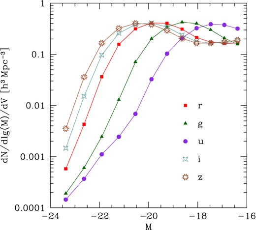
Luminosity function of semi-analytic galaxies in the MXXL simulation, in the five SDSS bands r, g, u, i, z. Note that artefacts produced by the finite mass resolution of the simulation are evident for M ≥ −20 to −19.

Open in new tab Download slide

In the upper-left panel of Fig. 2, we present the relative abundance of central, satellite and orphan galaxies as a function of their red-band absolute magnitude. ‘Central’ galaxies reside at the centres of the main halo (subhalo), and are therefore the main galaxies of the friends-of-friends (FoF) haloes. ‘Satellite’ galaxies inhabit satellite subhaloes within the FoF haloes. ‘Orphan’ galaxies are satellite galaxies whose dark matter subhalo has been stripped down below the resolution limit of the simulation. The figure clearly shows that the brightest galaxies (M_r ≤ −18) are mostly centrals. The satellites with a resolved dark matter subhalo are sub-dominant for all magnitude bins, but dominate among satellite galaxies with M_r < −20. These features depend on the mass resolution of the simulation (see Fig. B1 for an analogous figure constructed from the higher resolution Millennium simulation). With a much higher mass resolution, central galaxies would dominate at any luminosity and there would be no orphan galaxies.

Figure 2.

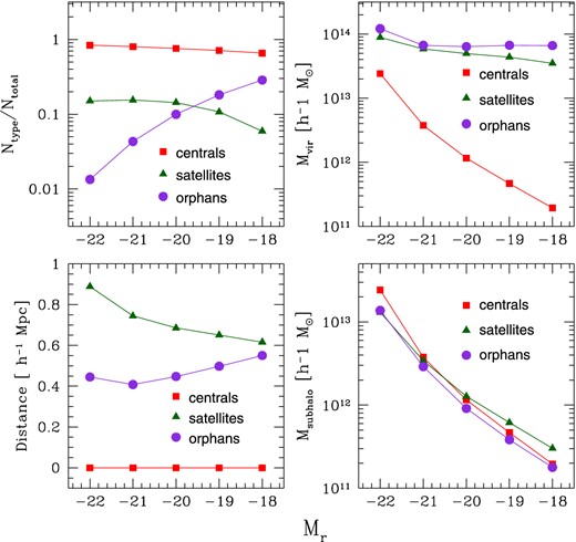
Galaxy properties as a function of absolute red-band magnitude. The galaxies are at redshift 0.24. Upper-left panel: the ratio of the number of galaxies of each type to the total number of galaxies in the respective magnitude bin. Upper-right panel: the virial mass of the host halo. Lower-left panel: the average distance of galaxies to the central galaxy. Lower-right panel: the mass of the subhaloes where the galaxies formed.

Open in new tab Download slide

The upper-right panel of Fig. 2 shows how the mass of the host haloes evolves with the galaxy luminosity. Independent of the brightness of satellite and orphan galaxies, the haloes hosting them are quite massive (M_vir ∈ [3 × 10¹³, 10¹⁴] h⁻¹ M_⊙), whereas the haloes inhabited by central galaxies display a substantial decrease in mass with decreasing luminosity. This drop in halo mass spans more than two orders of magnitude, starting at M ∼ 2 × 10¹³ h⁻¹ M_⊙.

The bottom-left panel of Fig. 2 shows the average distance of the galaxies from the central galaxy, as a function of magnitude. By definition, the distance of central galaxies is zero. Satellite galaxies are on average most distant from the halo centre: the brightest have a separation of ∼0.9 h⁻¹ Mpc, and the faintest of about 0.6 h⁻¹ Mpc. On the other hand, orphan galaxies are on average within [0.4, 0.6] h⁻¹ Mpc from the halo centre, which is a consequence of tidal forces being stronger closer to the halo centre where tidal disruption and mass-loss happen.

Finally, the bottom-right panel of Fig. 2 presents the evolution of the host subhalo mass with luminosity. For centrals, this is in fact the same as shown in the upper-right panel; the other two types follow the same trend as the centrals. Note that the subhalo mass associated with the orphan galaxies is defined to be the mass of the last subhalo tracked before it fell below the mass resolution of the simulation. We can see that there are no strong differences among different types which is a consequence of the fact that the r-band magnitude mostly traces the total amount of mass in stars, which in turn depends primarily on the total amount of gas available for star formation and thus on the mass of the host dark matter structure.

In this paper, we shall use only the red band, since most of the GGL and GC studies to date have focused on this band. We shall only consider galaxies with M_r < −19, split into four absolute-magnitude bins, with each bin spanning a single unit of magnitude, except for the brightest bin for which we take all galaxies with M_r < −22. We have ensured that above the chosen limit M_r < −19, our results are qualitatively insensitive to the finite mass resolution of the MXXL by explicitly comparing the GGL and GC signals with those derived from the higher-resolution Millennium simulation.

5 RESULTS I: CLUSTERING AND LENSING MEASUREMENTS IN MXXL

5.1 Methodology for estimating the projected correlation functions

In order to estimate the GGL and GC signals and their covariance from the MXXL data, we divide the simulation box into 216 subcubes of volume V_sub = [500 h⁻¹ Mpc]³. Each subcube therefore contains ≈1.4 × 10⁹ dark matter particles, as well as galaxies from the catalogues described in Section 4. For our analysis, we assume both the Born and Limber approximations, which allow us to perform all of the computations at the fixed redshift z = 0.24. For each of the subcubes, we measure the projected matter–matter, galaxy–matter and galaxy–galaxy correlation functions. In order to handle the huge data volume, we have developed a fast k-D tree code in c++ with MPI parallelization. Our algorithm is similar to that described by Moore et al. (2001) and Jarvis, Bernstein & Jain (2004). However, rather than invoking an approximate scheme for binning the pair counts as is done in these algorithms, we place every particle exactly into the correct radial bin. We have carefully tested that our code obeys the pair counting scaling DD ∝ t^3/2 and that it reproduces exactly the answer obtained from a brute-force pair summation code.

For the particular problem of computing the correlation functions in the MXXL simulation, we count pairs in logarithmic bins of the transverse distance R, and linear bins of the line-of-sight distance χ. Since the subcubes do not have periodic boundary conditions, we also cross-correlate the data with a random catalogue to account for boundary effects on the pair counts. With the pair counts for the (R, χ) bins, the 3D correlation function can be estimated by using the unbiased and minimum-variance (in the limit of no-clustering) estimator of Landy & Szalay (1993):

\begin{equation} \hat{\xi }=(D_1D_2-D_1R-D_2R+RR)/RR, \end{equation}

(35)

where D₁ and D₂ represent the first and second data catalogues, and R is the random catalogue. D₁D₂, D₁R, D₂R and RR represent the respective pair counts. For auto-correlations, D₁ = D₂, while for cross-correlations e.g. of galaxies and matter, they differ. Note that this estimator perfectly matches the one we defined in equations (A15) and (A18), since we took the weights there to be constant. The ratio of the number of data particles to the number of particles from the random catalogue represents the α from equation (A15). Some details of how we estimate these correlations are as follows. In order to obey computing time constraints, we limit the random catalogues to 10⁶ particles. To maintain a value as low as possible for α, we subsample both the matter and the galaxy data. The number of subsamples is 32, and for each of them we generate a random catalogue. The rate of sampling for matter is 1/4000, which gives us about 350 000 dark matter particles per subsample, while for each luminosity bin we randomly select no more than 150 000 galaxies. These values correspond to α ∼ 0.3 for matter and α ∼ 0.15 for galaxies in each luminosity bin. The only exception is the first luminosity bin, containing the brightest galaxies, which has only about 20 000 galaxies per subcube, and is therefore not subsampled. The matter particles and galaxies from every subsampled subcube are correlated with the random catalogue generated for that subsample. Thus, for all the subcubes, the ith subsample is correlated with the ith random catalogue. We have checked that given the number of data particles, the number of random particles is sufficiently large not to yield significant errors in the measured projected correlations.

We found that it was crucial to correct the projected correlation functions for the integral constraint, otherwise the results exhibited a strong dependence on the projection length χ_max. This owes to the fact that the total density of objects in each subcube is not guaranteed to reach the universal mean.

We implement the integral constraint in the estimates of the 3D galaxy correlation function in a similar fashion to the procedure described in Landy & Szalay (1993). To begin, we define the ‘geometric factor’:

\begin{equation} G_p(R_i, \chi _j)\equiv \frac{RR_{i j}}{\sum _{i,j} RR_{i j}\,{\rm d}V_{i j}} \,, \end{equation}

(36)

where RR_ij is the number of random pair counts for the bin (R_i, χ_j) and dV_ij is the cylindrical volume of the respective bin, i.e. |${\rm d}V_{ij}=\pi (R_{i+1}^2-R_i^2)\Delta \chi _j$|⁠, with Δχ_j ≡ χ_j+1 − χ_j. Thus, G_p(R_i, χ_j) is the number of pairs possible in the bin ij relative to the total number of pairs in the survey volume. It is normalized to unity over the survey volume, i.e. ∑_{i, j}G_p(R_i, χ_j)dV_ij = 1. The integral constraint is defined by the equation:

\begin{equation} \sum _{i,j} (1+\widehat{\xi }_{i j})G_p(R_i,\chi _j)\, {\rm d}V_{i j}\equiv 1+\xi _{V_s}, \end{equation}

(37)

where |$\widehat{\xi }_{i j}$| is the estimator introduced in equation (35) at the respective bin. The integral-constraint-corrected estimator for the projected galaxy correlation function is given by

\begin{equation} \widehat{w}_{\rm corr}(R_i)=\sum _{j=1}^{N_\chi } \left[\frac{1+\widehat{\xi }_{i j}}{1+\xi _{V_s}}-1\right]\Delta \chi _j, \end{equation}

(38)

where N_χ is the number of bins in χ. We apply this to all of the measurements.

Finally, we mention the choice of bins: we have 25 logarithmic bins in R, spanning the interval [0.04, 54] h⁻¹ Mpc, and 10 linear bins in χ, with a chosen χ_max of 100 h⁻¹ Mpc. We checked that the number of line-of-sight bins is sufficiently large to obtain an accurate estimation of the projected correlation function.

To summarize: the projected correlation functions are estimated through the following steps: (i) use the tree code to evaluate the 3D pair counts for each (R, χ) bin, and for every subsample; (ii) build the Landy–Szalay estimator for the 3D correlation function from the pair counts and determine the integral constraint factor; (iii) add the line-of-sight bins to obtain the projected correlation functions, i.e. compute |$\widehat{w}_{\rm corr}$| following equation (38); (iv) calculate the average of the subsamples.

5.2 Galaxy and matter correlation functions

Fig. 3 presents the projected matter–matter, galaxy–matter and galaxy–galaxy correlation functions – red, green and blue solid lines, respectively – from the 216 subcubes of the MXXL. Each line corresponds to the estimate from one subcube, and each panel to a magnitude bin, starting with the brightest galaxies in the upper-left corner, and down to the faintest in the lower-right corner. The measurements have some scatter for the two brightest magnitude bins, but are relatively tight otherwise. This plot also provides a check that none of the subcubes displays any anomalous behaviour.

Figure 3.

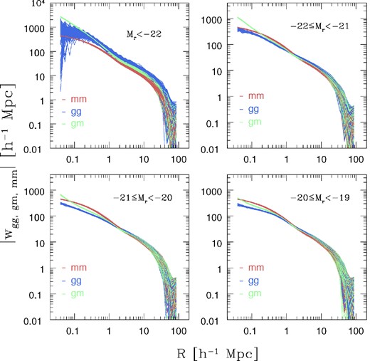
Projected correlation functions measured for all 216 subcubes of the MXXL at redshift 0.24. The red, blue and green lines represent the matter–matter, galaxy–galaxy and galaxy–matter correlation functions, respectively. In each panel, the galaxies are binned according to their r-band absolute magnitudes.

Open in new tab Download slide

5.3 Galaxy bias and cross-correlation coefficient

We may obtain the galaxy bias parameter either from the galaxy–galaxy or galaxy-matter projected correlation functions through

\begin{eqnarray} b_{\rm gg}(R) & = & \sqrt{\frac{w_{\rm gg}(R)}{w_{\rm mm}(R)}} \ ; \end{eqnarray}

(39)

\begin{eqnarray} b_{\rm gm}(R) & = & \frac{w_{\rm gm}(R)}{w_{\rm mm}(R)}\,. \end{eqnarray}

(40)

Fig. 4 presents the two bias estimates for all magnitude bins and averaged over all 216 subcubes of the MXXL simulation. There are several points worth noticing in these figures. First, on large scales, we see that both b_gg and b_gm appear to be constant and qualitatively consistent with one another. We also note that the bias is relatively similar for the fainter bins, but it increases sharply for the brightest galaxies. This luminosity dependence of the bias in SAM models is consistent with earlier studies (see Smith 2012, and references therein), and can be understood from Fig. 2. There we see that it is only for the brightest magnitude bin that the host haloes of both the central and satellite galaxies are very massive. For the fainter bins, the mass of the host haloes decreases with luminosity in the case of central galaxies, while remaining relatively constant in the case of the satellites. Thus, the bias of the latter is boosted. This explanation is consistent with the picture where an individual galaxy inherits the bias of the halo hosting it.

Figure 4.

The average galaxy bias for the various absolute-magnitude bins. The violet filled pentagons depict the bias computed as in equation (39), while the green symbols show the bias estimated as in equation (40). The error bars correspond to errors on the mean of the 216 subcubes.

Open in new tab Download slide

On smaller scales, we notice that b_gm > b_gg: the scale where this transition occurs decreases with increasing absolute magnitude, ranging from R ∼ 1 h⁻¹ Mpc for the brightest galaxies to R ∼ 0.07 h⁻¹ Mpc for the faintest bin. The fact that b_gm > b_gg can be qualitatively understood from the following reasons. The 3D galaxy–galaxy correlations in SAM models obey an exclusion condition, which is that individual galaxies cannot come closer than the separation of the sum of their individual subhalo virial radii. On scales smaller than this, the correlation function drops to −1. Whereas for the galaxy–matter cross-correlation function, no such exclusion is present and one simply probes the density profile of matter around galaxies – which is known to be cuspy (Hayashi & White 2008). However, in projection these effects are less significant, but nevertheless still operate and lead to the shape shown in Fig. 4. The transition scale varies with magnitude because the halo mass of central galaxies decreases with increasing absolute magnitude (cf. Fig. 2).

The cross-correlation coefficient can be defined as

\begin{equation} r_{\rm gm}(R)\equiv \frac{w_{\rm gm}(R)}{\sqrt{w_{\rm gg}(R)\,w_{\rm mm}(R)}} \equiv \frac{b_{\rm gm}(R)}{b_{\rm gg}(R)}. \end{equation}

(41)

Note that this is not the same as is usually understood in statistics, where the cross-correlation coefficient of two variables X and Y is constrained to be |r| ≤ 1. Equation (41) is defined in terms of correlation functions, and hence provided R ≠ 0 it is not required to obey the condition |r| ≤ 1. Indeed, if either the galaxy–galaxy or matter–matter correlation functions cross zero, which they most certainly do, then r is formally divergent. Nevertheless, the diagnostic properties of r are key: if the galaxy bias were linear and deterministic, then r = 1, and measurements of either w_gm or w_gg may be directly related to the underlying matter distribution, modulo an amplitude factor. However, any departure from unity indicates that the bias is either non-linear or stochastic, or both (for more discussion, see Dekel & Lahav 1999; Seljak & Warren 2004).

Fig. 5 shows the cross-correlation coefficient as a function of the transverse scale R. We find that on large scales, the correlation coefficient approaches unity for the four magnitude bins that we have considered. This implies that, at least for the SAM galaxies in MXXL, the large-scale bias is linear and deterministic and that it describes both the galaxy–galaxy and galaxy–matter correlation functions. On small scales, we see that the correlation coefficient decreases sharply and then shoots up above unity. This is consistent with the non-linear scale-dependent bias presented in Fig. 4. Note that the small-scale clustering of galaxies is very sensitive to the treatment of dynamical friction of orphan galaxies, so we do not wish to overinterpret the results of Figs 4 and 5 for R < 100 h⁻¹ kpc.

Figure 5.

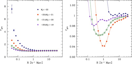
The average cross-correlation coefficient, e.g. equation (41) as a function of transverse radius. Left-hand panel: the full range.Right-hand panel: zoom-in.

Open in new tab Download slide

5.4 Comparison of the measured and theoretical projected galaxy correlation function

In Fig. 6, we show again the projected galaxy correlation functions for the four magnitude bins, but this time we have averaged the data over the 216 MXXL subcubes. The error bars are plotted on the mean. The solid lines present the theoretical predictions. We evaluate the theory as follows: instead of a direct numerical evaluation of equation (26), which would require a model for P_gg(k), we determine the projected non-linear matter correlation function under the Limber approximation by replacing P_gg → P_mm(k). We then simply multiply this quantity by the measured bias, e.g. equation (39):

\begin{equation} w^L_{\rm gg}(R) = b_{\rm gg}(R) w^L_{\rm mm}(R) \,. \end{equation}

(42)

In computing |$w^L_{\rm mm}$|⁠, we use the non-linear matter power spectrum fitting formula halofit (Smith et al. 2003).

Figure 6.

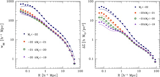
Left-hand panel: the projected galaxy correlation function for various magnitude bins. The symbols denote the average of the 216 subcubes; the error bars are on the mean. The lines represent the theoretical predictions of equation (26). Right-hand panel: the excess surface density. Symbols and lines are just like in the left-hand panel.

Open in new tab Download slide

In Fig. 6 we see that on small scales R < 0.1 h⁻¹ Mpc, the predictions underestimate the measured w_gg by roughly ∼20 per cent. These discrepancies are attributed to the fact that halofit underpredicts the true non-linear matter power spectrum on small scales (Takahashi et al. 2012). The more recent work of Fosalba et al. (2015a,b) shows however that the revised halofit of Takahashi et al. (2012) overpredicts the non-linear power spectrum and consequently also the convergence power spectrum on small scales. Since the agreement between halofit models and simulation measurements depends on both the mass resolution and the volume of the simulations – the closer the simulations’ specifications to those used for the calibration of the semi-analytical prescriptions, the better the agreement – we defer more sophisticated theory predictions to a future work and are satisfied for now that the original halofit of Smith et al. (2003) gives reasonable enough answers for our purpose here.

It is also interesting to note that the faintest galaxies yield high projected correlation functions around 1 h⁻¹ Mpc, most likely due to contributions from the satellite galaxies, which inhabit higher mass haloes and are therefore more biased.

5.5 The stacked tangential shear of galaxies

As mentioned earlier, since the full particle data were not available for a large set of redshifts, we were not able to perform ray-tracing simulations. Instead, we use the Born approximation to make lensing observables from the MXXL data. In real terms, this means that the convergence is obtained as a weighted line-of-sight integration of the matter density fluctuations (Bartelmann & Schneider 2001):

\begin{equation} \kappa ({\boldsymbol \theta}) = \frac{3H_0^2\Omega _{\rm m}}{2c^2} \int _{0}^{\chi } {\rm d}\chi ^{\prime } \frac{\chi ^{\prime }(\chi -\chi ^{\prime })}{\chi } \frac{\delta (\chi ^{\prime } {\boldsymbol \theta},\chi ^{\prime })}{a(\chi ^{\prime })} \,, \end{equation}

(43)

where we have assumed a flat space–time geometry and H₀ is the Hubble constant, c is the speed of light, δ is the linear matter density perturbation and a is the expansion factor.

If we now reexamine equation (15), it can be proven that the azimuthally averaged tangential shear about a randomly selected point |${\boldsymbol \theta}_0$|⁠, which we take to be |${\boldsymbol 0}$|⁠, may be written in real space as (Schneider 2005)

\begin{equation} \gamma _{t,a}(\theta ) = \overline{\kappa }(\theta ) -\kappa _a(\theta ) \,. \end{equation}

(44)

If instead of random points we consider the centre of a lens galaxy as the reference point, then on averaging over all galaxies the above expression becomes (Guzik & Seljak 2001)

\begin{equation} \left\langle \widehat{\gamma }_{t,a}^g(R, z_{\rm l}, z_{\rm s})\right\rangle =\frac{\langle \widehat{\Delta \Sigma } (R, z_{\rm l})\rangle }{\Sigma _{\rm crit}(z_{\rm l}, z_{\rm s})} \,, \end{equation}

(45)

where we used the relation θ = R/χ(z_l) and the differential surface mass density is given by

\begin{equation} \widehat{\Delta \Sigma }(R, z_{\rm l}) = \rho _{\rm m}^0 \left[\widehat{\overline{w}}_{\rm gm}(<R, z_{\rm l})-\widehat{w}_{\rm gm}(R, z_{\rm l})\right]. \end{equation}

(46)

In the above, |$\rho _{\rm m}^0$| is the comoving matter density of the Universe, and we have assumed that the circularly averaged tangential shear is sourced only by the matter associated with a single lens galaxy. The critical surface density for lensing is given by

\begin{eqnarray*} \Sigma _{\rm crit}(z_{\rm l}, z_{\rm s}) \equiv \frac{c^2}{4\pi G}\frac{D_{\rm A}(z_{\rm s})}{D_{\rm A}(z_{\rm l};z_{\rm s}) D_{\rm A}(z_{\rm l})},{\nonumber } \end{eqnarray*}

where D_A(z_s), D_A(z_l) and D_A(z_l; z_s) represent the observer–source, observer–lens and lens–source angular diameter distances, respectively. To keep the notation compact, we shall omit the dependence on z_l, z_s and write the critical density simply as Σ_crit.

From our earlier discussion in Section 2.2, we see that an alternative way to compute the stacked tangential shear is through equation (15). In the Limber approximation and assuming once again that only matter associated with the lens galaxy creates the shear signal, we have

\begin{equation} \left\langle \widehat{\gamma }_{t, a}^g(R, z_{\rm l}, z_{\rm s})\right\rangle =\frac{\rho _{\rm m}^0}{\Sigma _{\rm crit}} \int \frac{{\rm d}^2 k_\perp }{(2\pi )^2}\mathcal {P}_{\rm gm} (k_\perp , z_{\rm l}) J_2(k_\perp R). \end{equation}

(47)

We shall use equation (46) to compute the excess surface density both analytically and from the simulation data. For the theoretical predictions, we choose to compute w_gm in the same way as we computed w_gg in equation (42), only this time using b_gm from equation (40). We prefer this approach to that offered by equation (47), because it allows us to obtain ΔΣ in the same way for both simulations and the theory. At larger R this choice is unimportant; however, at smaller radii, owing to the fact that the radial binning does not start at R = 0, it plays a more important role and the results from equations (45) and (47) differ systematically.

The right-hand panel of Fig. 6 presents a comparison between the theoretical predictions and measurements of ΔΣ as a function of the transverse spatial scale R, for the four magnitude bins considered. The symbols correspond to the simulations and the lines to the theory predictions. On large scales, R > 10 h⁻¹ Mpc, we see that similar to w_gg, the shear amplitudes in the three faintest bins are comparable, whereas the brightest galaxies have a higher amplitude. On smaller scales, R < 0.5 h⁻¹ Mpc, we find a systematic trend: the brighter the galaxies, the larger the amplitude of the tangential shear profile. This finding is in accord with the GGL measurements from the SDSS by Mandelbaum et al. (2006a).

On closer inspection of the faintest luminosity bin, we see that it appears to have a somewhat broad, flattish shear profile, with a very slight second peak at ∼1 h⁻¹ Mpc, and higher amplitude than the brighter bins (excepting the brightest bin) on intermediate scales 2 < R < 10 [ h⁻¹ Mpc]. This might be due to the increased relative abundance of satellite galaxies compared to centrals. The satellite galaxies are mainly hosted by high-mass haloes and have an average distance from the centre of the main halo that is roughly of the order of ∼0.5 h⁻¹ Mpc, and so we expect that their tangential shear profiles receive two significant contributions: the first from the dark matter associated with their own subhalo; the second comes as the shear profile radius encompasses the central cusp of the main halo. This qualitatively explains the broadening of the profile of the faintest bin. We also note that the theory underpredicts the measurements more significantly than for w_gg. This can be attributed to the small-scale inaccuracies of halofit contributing to |$\overline{w}_{\rm gm}(<\!\!R)$| at all radii.

6 RESULTS II: COVARIANCE MATRICES FROM THE MXXL

6.1 Covariance of the projected correlation function

In Fig. 7, we present the errors on the mean projected galaxy correlation function, divided through by the signal, as a function of the transverse scale R, and for the magnitude bins discussed previously. The blue pentagons in the figure represent the noise-to-signal ratio estimated directly from the N = 216 subcubes. The unbiased estimator of the mean and covariance is

\begin{equation} \left\langle\widehat{\overline{w}}_{\rm gg}(R_i)\right\rangle \equiv \frac{1}{N} \sum _{k=1}^{N}\widehat{\overline{w}}_{\rm gg,k}(R_i), \end{equation}

(48)

\begin{eqnarray} {\rm Cov}[\widehat{\overline{w}}_{\rm gg}](R_i, R_j) & & \equiv \frac{1}{N-1} \sum _{k=1}^{N} \left[\widehat{\overline{w}}_{\rm gg,k}(R_i) -\left\langle\widehat{\overline{w}}_{\rm gg}(R_i)\right\rangle\right] {\nonumber }\\ & & \times \left[\widehat{\overline{w}}_{\rm gg,k}(R_j) -\left\langle\widehat{\overline{w}}_{\rm gg}(R_j)\right\rangle\right], \end{eqnarray}

(49)

where |$\widehat{\overline{w}}_{\rm gg,k}$| is the bin-averaged estimate of the projected correlation function from the kth subcube. The covariance and error on the mean are then simply obtained by further dividing the right-hand side of equation (49) by the number of subcubes N. The red triangles denote the predictions obtained from direct evaluation of equations (26) and (32), where we scaled the variance to the entire MXXL volume.

Figure 7.

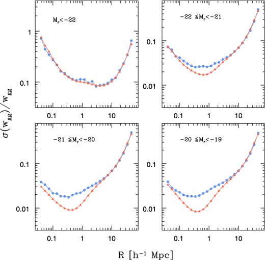
The noise-to-signal for the projected galaxy correlation function. The red triangles represent the theory prediction, and the blue pentagons the simulation measurements.

Open in new tab Download slide

The theoretical predictions for the brightest galaxies agree extremely well with the measured errors. This owes to the fact that on large scales, R > 10 h⁻¹ Mpc, the errors are determined by the Gaussian part of the variance. On smaller scales, these objects are relatively sparse, and so the shot-noise contribution to the variance quickly dominates. Both of these two limits are well characterized by our formula.

For the fainter magnitude bins, there is reasonably good agreement between our model and the data on both large (R > 10 h⁻¹ Mpc) and small (R < 0.1 h⁻¹ Mpc) scales. The former is due to the prominence of Gaussian contributions on large scales, whereas the latter is due to the shot-noise dominance on small scales. However, on intermediate scales (0.1 < R < 1 h⁻¹ Mpc), the agreement is not so good, and we see that the data have errors roughly a factor of ∼2 larger than the predictions. This is to be expected, since for these scales the non-Gaussian corrections (e.g. the connected part of the trispectrum and also the bispectrum), which we neglected in deriving equation (32), are significant and have the effect of increasing the errors.

To compare the off-diagonal elements of the predicted and measured covariance from equations (32) and (49), we choose to examine the correlation matrix. For any covariance matrix |$ {C}[X]$|⁠, the correlation matrix |$ {r}[X]$| can be defined as

\begin{equation} r[X]_{i j}=\frac{C[X]_{i j}}{\sqrt{C[X]_{i i}\,C[X]_{j j}}}\,, \end{equation}

(50)

where the subscript X is a place-holder for the statistic. The correlation matrix obeys the constraint |r[X]_ij| ≤ 1, ∀i, j.

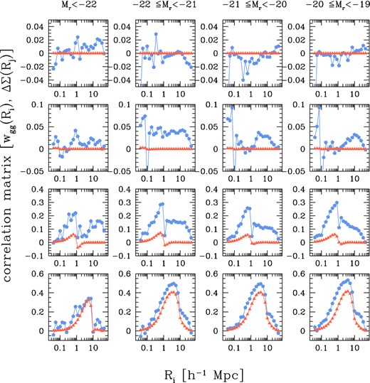
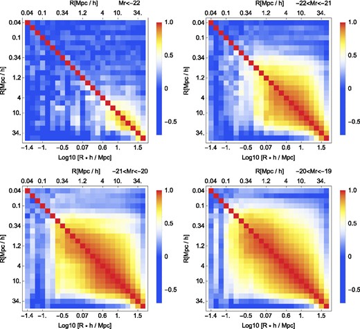
Fig. 8 shows four rows of the correlation matrix of |$ {r}[\widehat{\overline{w}}_{\rm gg}]$| at radii (R_i, R_j) as a function of R_j and at fixed radius R_i. The fixed scales correspond roughly to R_i = 0.04, 0.1, 1, 10 h⁻¹ Mpc, and in each panel can be quickly determined by noting that |$r[\widehat{\overline{w}}_{\rm gg}](R_i=R_j)=1$|⁠. From left to right, each column represents a magnitude bin.

Figure 8.

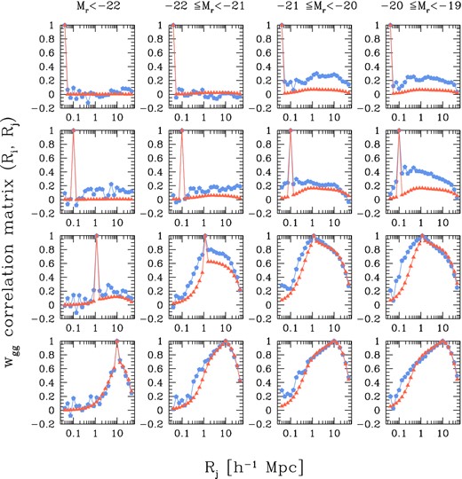
The correlation matrix from equation (50) for the projected galaxy correlation function. From top to bottom, the rows present four scales: R_i = 0.04, 0.1, 1, 10 h⁻¹ Mpc. From left to right, the columns depict the four magnitude bins, as indicated in each panel. The symbols are the same as in the previous figure.

Open in new tab Download slide

There are some notable trends: when the fixed scale R_i is large (bottom row of the figure), the neighbouring bins of the matrix are significantly correlated, and the strength of the correlations is |$r[\widehat{\overline{w}}_{\rm gg}]>0.5$|⁠. There is a decrease in the correlation coefficient as one considers brighter magnitude bins. These findings are in good agreement with our Gaussian model. When the fixed scale is small (R_i = 0.04 Mpc), for the brighter galaxy bins there is virtually no evidence for bin-to-bin correlations. Again this is consistent with the predictions of our model, and is attributed to the fact that for so few objects the shot-noise errors simply dominate. However, when we consider the intermediate scales (second and third rows of panels in the figure), the model predictions underestimate the bin-to-bin correlations that are exhibited by the data. We interpret this as a sign that the non-Gaussian contributions to the covariance matrix, which we have neglected in our model, are significant. For a more intuitive but less quantitative depiction of the GC correlation matrix, as well as the GGL one and their cross-correlation, we refer the reader to Figs 13–16.

6.2 Covariance of the stacked tangential shear

Fig. 9 presents the errors on the mean of the stacked tangential shear as a function of the transverse scale R. The blue pentagons in the figure represent the noise-to-signal ratio estimated directly from the 216 MXXL subcubes estimated through

\begin{equation} \left\langle \widehat{\overline{\gamma }}_t^g(R_i)\right\rangle \equiv \frac{1}{\Sigma _{\rm crit}}\frac{1}{N} \sum _{k=1}^{N} \widehat{\Delta \Sigma }_{k}(R_i), \end{equation}

(51)

\begin{eqnarray} {\rm Cov}[\widehat{\overline{\gamma }}_{t}^g](R_i, R_j) & & \equiv \frac{1}{\Sigma _{\rm crit}^2}\frac{1}{N-1} \sum _{k=1}^{N} \left[\widehat{\Delta \Sigma }_{k}(R_i)-\left\langle \widehat{\Delta \Sigma }_{k} (R_i)\right\rangle \right] {\nonumber }\\ & & \times \left[\widehat{\Delta \Sigma }_{k}(R_j)-\left\langle \widehat{\Delta \Sigma }_{k}(R_j)\right\rangle \right], \end{eqnarray}

(52)

where |$\widehat{\Delta \Sigma }_{k}(R_i)$| is the estimate of the excess surface density from the kth subcube.

Figure 9.

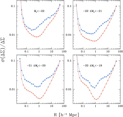
The noise-to-signal for the stacked tangential shear. The red triangles represent the theory predictions, while the blue pentagons correspond to the simulation measurements.

Open in new tab Download slide

Let us now turn to the theoretical predictions. We note that equation (29) can be rewritten for ΔΣ at the lens redshift z_l and using the Limber approximation as done in Section 3.2 and equation (47). In the following, we shall ignore the shape-noise contribution from equation (29), since the latter is not an issue for our measurements. What is an issue however, given that we determine the matter distribution from an N-body simulation of finite resolution, is the particle shot noise which accompanies |$\mathcal {P}_{\rm mm}$|⁠. We therefore write the final expression for the measured bin-averaged covariance of the excess surface density as

\begin{eqnarray} &&{{\rm Cov}\left[\widehat{\overline{\Delta \Sigma }}\right](R_i, R_j) = \frac{1}{A_{\rm s}}\left(\rho _{\rm m}^0\right)^2 \int \frac{{\rm d}^2k_\perp }{(2\pi )^2}\overline{J}_2(k_\perp R_i) \overline{J}_2(k_\perp R_j)} {\nonumber }\\ &&{\quad\times \left\lbrace \left[\mathcal {P}_{\rm mm}(k_\perp ) +\frac{1}{\bar{n}_p}\right] \,\left[\mathcal {P}_{\rm gg}(k_\perp )+ \frac{1}{\bar{n}_g}\right] + \mathcal {P}_{\rm gm}^2(k_\perp )\right\rbrace ,} \end{eqnarray}

(53)

where all the power spectra are taken at redshift z_l; the transverse area of the survey A_s was introduced in Section 3.2; |$\bar{n}_{\rm p}$| and |$\bar{n}_{\rm g}$| are the mean particle and galaxy densities in the simulation. The above covariance has dimension of L⁻⁴, as expected.

The theory predictions of equation (53) are presented as the red triangles in Fig. 9. As in the case of w_gg, we see that the agreement between theory and measurements is good on large (R > 10 h⁻¹ Mpc) and small (R < 0.1 h⁻¹ Mpc) scales. However, on intermediate scales the theory underestimates the true errors. We also notice that the predictions are increasingly poor for the fainter galaxies. For the brightest galaxies, the discrepancy at R ∼ 1 h⁻¹ Mpc is roughly a factor of ∼2, whereas for the faintest galaxies it is roughly ∼3. Thus, compared to w_gg, the predictions for the stacked shear seem worse, even for the shot-noise-dominated brightest galaxies. This suggests that the non-Gaussian contributions to the variance are more important for the stacked tangential shear than for the projected correlation function. However, in a real shear survey, this discrepancy may not be so crucial, since the addition of the shape-noise term will certainly be a strong source of noise on small scales. In Appendix C, we present a theoretical estimation of the impact of shape noise on the GGL variance and correlation matrix.

Fig. 10 presents four rows of the correlation matrix of |$\widehat{\overline{\gamma }}^g_t$| at {R_i, R_j} as a function of R_j and for fixed R_i, with the covariance estimated according to equation (52). The measurements are represented in the figure as the blue pentagons. The theoretical predictions are obtained by evaluating equation (53), and are denoted by the red triangles. The general trends are similar to those found in Fig. 8: on small scales (R_i = 0.04 h⁻¹ Mpc, i.e. the top row of the figure), the theory and measurements show weak bin-to-bin correlations and the measurements seem somewhat noisy. Qualitatively, they are consistent with uncorrelated noise. On large scales (R_i = 10.0 h⁻¹ Mpc, i.e. the bottom row of the figure), the measurements show significant bin-to-bin correlations. However, the correlations appear to be somewhat weaker than was found for the projected correlation function for more distant bins. In addition, the Gaussian predictions of our model do not describe these correlations as well as in the case of w_gg. On intermediate scales, 1 < R_i < 10[ h⁻¹ Mpc], the correlations are significantly stronger for all magnitude bins than predicted by our theoretical model. Once again, this suggests that the tangential shear signal is significantly more non-Gaussian on these scales than the projected galaxy correlation function.

The correlation matrix from equation (50) for the stacked tangential shear. Just like in Fig. 8, the rows present four scales: Ri = 0.04, 0.1, 1, 10 h−1 Mpc. From left to right, the columns depict results for increasingly fainter galaxies, as indicated in each panel.

Figure 10.

The correlation matrix from equation (50) for the stacked tangential shear. Just like in Fig. 8, the rows present four scales: R_i = 0.04, 0.1, 1, 10 h⁻¹ Mpc. From left to right, the columns depict results for increasingly fainter galaxies, as indicated in each panel.

Open in new tab Download slide

6.3 Cross-covariance of the projected correlation function and stacked tangential shear

In order to perform a joint likelihood analysis of the combination of the projected galaxy correlation function and the stacked tangential shear profile, one would start by writing the joint vector of measurements:

\begin{equation} {\boldsymbol X}^{\rm T} \!=\! \left( \frac{\widehat{\overline{w}}_{\rm gg}(R_1)}{\sigma [\widehat{\overline{w}}_{\rm gg}](R_1)}, \ldots , \frac{\widehat{\overline{w}}_{\rm gg}(R_{\mathcal {N}})}{\sigma [\widehat{\overline{w}}_{\rm gg}](R_{\mathcal {N}})}, \ldots \frac{\widehat{\overline{\gamma }}^g_t(R_{\mathcal {N}})}{\sigma [\widehat{\overline{\gamma }}^g_t](R_{\mathcal {N}})} \right), \end{equation}

(54)

where we have normalized the measurements by their diagonal errors, so as to obtain dimensionless numbers. |$\mathcal {N}$| is the number of transverse radial bins. Assuming a Gaussian likelihood, the normalized data would then be written as

\begin{equation} \log {\mathcal {L}}({\boldsymbol X}|{{\bf \phi}}) \ \propto \sum _{i,j=1}^{\mathcal {N}} [X_i-\bar{X}_i({{\bf \phi}})] \ r[X]^{-1}_{ij} \left[X_j-\bar{X}_j({{\bf \phi}})\right], \end{equation}

(55)

where |$\bar{X}_i({\bf \phi})$| is the expectation of the theoretical model and |$ {r}[X]^{-1}$| is the inverse correlation matrix. The correlation matrix is built from four blocks:

\begin{equation} {r}[X] = \left( \begin{array}{cc} {r}\left[\widehat{\overline{w}}_{\rm gg}\right] &\quad {r}\left[\widehat{\overline{w}}_{\rm gg},\widehat{\overline{\gamma }}^g_t\right] \\ {r}\left[\widehat{\overline{\gamma }}^g_t, \widehat{\overline{w}}_{\rm gg}\right] &\quad {r}\left[\widehat{\overline{\gamma }}^g_t\right] \end{array}\right), \end{equation}

(56)

where the off-diagonal blocks are simply the transpose of one another. Again, we see that |$\left| {r}_{X}\right|\le {1}$|⁠, i.e. the absolute value of the determinant must be less than unity, through the Cauchy–Schwarz inequality.

Figs 11 and 12 present four rows and columns through the off-diagonal block |$ {r}[\widehat{\overline{w}}_{\rm gg},\widehat{\overline{\gamma }}^g_t]$| of the full correlation matrix, respectively. Note that unlike the other block matrices, the off-diagonal block is not symmetric, hence the need to examine the columns as well as the rows. Just like before, the blue pentagons denote the measurements from the 216 MXXL subcubes. The cross-covariance was estimated similarly to equations (49) and (52):

\begin{eqnarray} {\rm Cov}\left[\widehat{\overline{w}}_{\rm gg}, \widehat{\overline{\gamma }}_{t}^g\right](R_i, R_j) &\!\equiv\! &\frac{1}{\Sigma _{\rm crit}}\frac{1}{N\!-\! 1} \sum _{k=1}^{N} \!\left[\widehat{\overline{w}}_{\rm gg,k}(R_i) \!-\!\left\langle\widehat{\overline{w}}_{\rm gg}(R_i)\right\rangle\right] {\nonumber }\\ &&{\times}\; \left[\widehat{\Delta \Sigma }_{k}(R_j)-\left\langle \widehat{\Delta \Sigma }_{k}(R_j)\right\rangle \right]. \end{eqnarray}

(57)

Owing to the fact that we use the excess surface mass density as a proxy for tangential shear, we may rewrite equation (34) as

\begin{eqnarray} {\rm Cov}\left[\widehat{\overline{w}}_{\rm gg}(R_i), \widehat{\overline{\Delta \Sigma }}(R_j)\right] & & = \frac{2 \rho _{\rm m}^0}{A_{\rm s}} \int \frac{{\rm d}^2k_{\perp }}{(2\pi )^2} \overline{J}_0(k_\perp R_i) \overline{J}_2(k_\perp R_j) {\nonumber }\\ & &{\times} \mathcal {P}_{\rm gm}(k_\perp )\left[\mathcal {P}_{\rm gg}(k_\perp ) +\frac{1}{\bar{n}_{\rm g}}\right]. \end{eqnarray}

(58)

The theoretical predictions from this expression are presented in Figs 11 and 12 as the red triangles.

Figure 11.

The cross-correlation matrix of the projected galaxy correlation function and the stacked tangential shear. As in Figs 8 and 10, the rows present four scales: R_i = 0.04, 0.1, 1, 10 h⁻¹ Mpc. From left to right, the columns depict the galaxy bins with decreasing brightness.

Open in new tab Download slide

The cross-correlation matrix of the projected galaxy correlation function and the stacked tangential shear, this time fixing Rj = 0.04, 0.1, 1, 10 h−1 Mpc.

Figure 12.

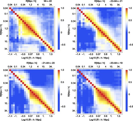
The cross-correlation matrix of the projected galaxy correlation function and the stacked tangential shear, this time fixing R_j = 0.04, 0.1, 1, 10 h⁻¹ Mpc.

Open in new tab Download slide

On small scales (R < 0.1 h⁻¹ Mpc, i.e. the top row of the figures), we see that for all of the magnitude bins considered, the cross-correlation coefficient is small (r < 0.2), and reasonably consistent with the theoretical predictions from equation (58). On large scales (R ∼ 10 h⁻¹ Mpc, i.e. the bottom row in the figures), the cross-correlation coefficient is larger, with r ∼ 0.8 for some of the bins. Also, the theoretical predictions are qualitatively in agreement, although the measurements do show a stronger degree of correlation. On intermediate scales (the middle two rows), the measurements show stronger bin-to-bin correlations than predicted by the theory. These correlations on intermediate to large scales are important to include in any joint likelihood analysis of GC and GGL. Otherwise, the likelihood search may lead to biased and overoptimistic parameter constraints.

6.4 Testing the jackknife method to estimate covariances

We now want to see how the correlation matrices estimated from the entire MXXL data compare to those evaluated through the jackknife method.

We pick one of the subcubes of the simulation, and generate 64 jackknife samples by removing a region of the subcube and estimating the projected correlation functions from the remaining data. The regions that are removed are in the shape of a rectangular parallelepiped, with the long side aligned with the |${\hat{\boldsymbol z}}$| direction of the subcube, i.e. the projection direction, and the shorter sides describing a square in the |${\hat{\boldsymbol x}}{\rm -}{\hat{\boldsymbol y}}$| plane. The latter is obtained by dividing the subcube side into eight equal segments along both |${\hat{\boldsymbol x}}$| and |${\hat{\boldsymbol y}}$| directions, resulting in 64 adjacent squares. Thus, the dimensions of each parallelepiped are 62.5 × 62.5 × 500 [ h⁻¹ Mpc]³.

The rest of the calculations follow the same path as detailed in Section 5.1. Each jackknife sample requires its own random catalogue. Just as before, the galaxies and dark matter particles are subsampled 32 times, in order to reduce the shot noise and the α parameter describing the relative density of the simulation and random data. The resulting correlation functions are the average of the 32 subsample measurements. Once the projected correlation functions and excess surface density are computed for each jackknife sample, we combine them to estimate the covariance matrices for ΔΣ and w_gg:

\begin{eqnarray} {\rm Cov}\left[\widehat{X}, \widehat{Y}\right](R_i, R_j) &=&\frac{N_{\rm samp}-1}{N_{\rm samp}} \sum _{k=1}^{N_{\rm samp}} \left[\widehat{X}_k(R_i) - \left\langle \widehat{X}_k(R_i)\right\rangle \right] {\nonumber }\\ &&{\times}\, \left[\widehat{Y}_k(R_j) - \left\langle \widehat{Y}_k(R_j)\right\rangle \right] \,, \end{eqnarray}

(59)

where N_samp = 64; X and Y stand for w_gg and ΔΣ, and the mean is the average of the jackknife samples:

\begin{equation*} \left\langle \widehat{X}(R)\right\rangle = \frac{1}{N_{\rm samp}} \sum _{k=1}^{N_{\rm samp}} \widehat{X}_k(R) \,. {\nonumber } \end{equation*}

In Fig. 13, we present a comparison between our original measurement of the correlation matrix of w_gg and the one obtained through jackknife resamplings, for the four magnitude bins that we have considered. In each panel, the upper-right half depicts the original correlation matrix, while the lower left shows the jackknife result. The agreement is remarkable, with the jackknife result being slightly noisier than the full one. Similarly, Fig. 14 shows the same comparison for the excess surface density. Figs 15 and 16 present the original and jackknife cross-correlation matrices, respectively. In all figures the jackknife result appears a little more correlated than the original measurement, but in general the agreement is surprising. Although not shown, we have also compared the variance for w_gg and ΔΣ: the findings were very similar, with the jackknife variance being a little noisier, but essentially matching the original measurement rather well.

Figure 13.

The correlation matrix of w_gg for the four magnitude bins considered. The upper-right triangle of the matrix represents the correlation matrix measured from the whole simulation, i.e. the same as in Fig. 8. The lower-left triangle is the correlation matrix obtained from jackknife samplings of one of the subcubes of the simulation.

Open in new tab Download slide

Figure 14.

The same as in the previous figure, only for the case of ΔΣ.

Open in new tab Download slide

Figure 15.

The cross-correlation matrix of w_gg and ΔΣ, as computed from the whole MXXL data and presented also in Figs 11 and 12.

Open in new tab Download slide

Figure 16.

The jackknife cross-correlation matrix of w_gg and ΔΣ, estimated from 64 samplings of one of the MXXL subcubes.

Open in new tab Download slide

7 CONCLUSIONS

In this paper, we have explored the required ingredients for performing a joint likelihood analysis of GC and GGL. The combination of these probes has the potential to enable simultaneous constraints of the cosmological and galaxy formation model parameters.

In Section 2, we developed an analytic framework to predict the projected correlation function and the stacked tangential shears of a population of galaxies. We provided both exact and Limber-approximated expressions for the observables in the flat-sky limit. In Appendix A, we presented the full derivations of the auto- and cross-covariance matrices. In Section 3, we summarized the results for the case where the underlying density fluctuations are Gaussian and modulated by a shot-noise contribution. The two necessary ingredients for the results of Sections 2 and 3 are the galaxy–galaxy and galaxy–matter power spectra or alternatively a model for the bias defined by equations (39) and (40).

The theoretical predictions of the models were then tested against measurements from numerical simulations of structure formation. In Section 4, we provided a brief overview of the MXXL simulation. The galaxy catalogues were generated using the Garching SAM of galaxy formation, which enabled us to compute the u, g, r, i, z SDSS absolute magnitudes. As a diagnostic of the SAM galaxies we presented the evolution of the GLF for the five bands. We also explored certain properties of the galaxies as a function of absolute r-band magnitude (M_r), allowing us to understand the impact of the finite mass resolution of the MXXL simulation on the derived galaxy properties. Through detailed comparison with the Millennium simulation, we determined that resolution effects were qualitatively important only for magnitudes fainter than M_r > −19.

In Section 5, we described our methods for estimating the projected correlations from the MXXL. This required the implementation of fast and efficient algorithms, since the dark matter distribution was represented by over 300 billion dark matter particles and the galaxy catalogue contained more than a billion objects. We thus developed a parallel k-D tree algorithm for computing the correlation functions of the subsampled matter and galaxy distributions.

We split the galaxy catalogues into four subsamples based on their M_r, with the constraint that M_r < −19. We also sliced the dark matter and galaxy catalogues into a series of 216 subcubes of volume 500 h⁻³ Mpc³. As a step towards modelling the GC and GGL signals, we examined the projected galaxy–galaxy and galaxy-mass correlation functions using the estimator proposed by Landy & Szalay (1993). We also computed the bias coefficients as a function of scale from these statistics. We found that on large scales, R > 10 h⁻¹ Mpc, the bias was consistent with being linear and deterministic. On smaller scales, the bias possessed a complex scale dependence, which varied with the magnitude bin through the larger number of satellites and their spatial distribution, as well as the decreasing host mass for the centrals in the fainter bins. We also found that the cross-correlation coefficient was significantly greater than unity on small scales. This could be explained as a consequence of an exclusion effect – no two galaxies may be closer than the sum of their respective virial radii.

We next computed the excess surface mass density ΔΣ, which is directly proportional to the tangential shear, and the projected galaxy correlation function for each of the magnitude bins and for each of the 216 subcubes. These were compared to the theoretical predictions in the Limber approximation. The evaluation of the theory required a model for the non-linear matter power spectrum and the scale dependence of the bias. For the former, we used the halofit code (Smith et al. 2003), and for the latter we took directly the measured bias. We found that on small scales the theory underpredicted the measurements by ≲20 per cent for w_gg and by ≲30 per cent for ΔΣ. This was attributed to the diminished accuracy of halofit on small scales. Both functions displayed complicated features for galaxies in the faintest magnitude bin M_r > −20. This was again attributed to the increased abundance of satellite galaxies.

In Section 6, we used the measured estimates of w_gg and ΔΣ from the subcubes to construct the auto- and cross-covariance matrices. We found that on large and small scales the errors were reasonably well described by the Gaussian plus shot-noise model. However, on intermediate scales, 0.1 < R < 10 h⁻¹ Mpc, the measured errors were significantly larger by a factor of ∼2–3. This suggests that in order to accurately model the covariance matrix one needs to take account of the non-Gaussian contributions from the bi- and trispectrum. Note that in the case of GGL, the presence of shape noise does alleviate some of the non-Gaussianities on intermediate scales, as shown in Appendix C.

Finally, we compared the auto- and cross-covariances obtained from the jackknife samplings of one of the subcubes of MXXL with the full simulation covariances. We concluded that the jackknife method is remarkably effective, for both auto- and cross-covariances.

Importantly, we found that the cross-covariance between w_gg and ΔΣ was not zero. The elements of the cross-covariance matrix showed significant bin-to-bin correlations with r ∼ 0.8 for some elements on large scales. This result is important, since in a number of previous analyses we neglected the cross-correlation of GC and GGL. Our results suggest that if these correlations are ignored, then a standard likelihood analysis would lead to biased and overoptimistic constraints on the parameters of the models.

In the future, more work will be required to establish an accurate model of the GC and GGL signals on scales R < 5 h⁻¹ Mpc. We note that, whilst the SAM model of galaxy formation is not to be taken as an exact replica of reality, it nevertheless captures many of the effects that we expect to have to model when constraining model parameters with real data. It will also be important to determine how well the combination of GC and GGL can actually break the degeneracies between the galaxy formation and cosmological parameters. We shall aim to explore this in a future paper. In the meantime, we note that Eifler et al. (2014) have explored clustering and lensing probe combinations and have included additional non-Gaussian terms in the modelling of the covariances. However, they have assumed a rather simplistic modelling of the galaxy bias, which we showed here is not the case. This leads us to suspect that their results will be somewhat overoptimistic.

Another possibility is the exploration of the ϒ statistic (Baldauf et al. 2010; Mandelbaum et al. 2013), which was developed to remove the complicated scale dependences of the bias. However, what is not clear is whether the ϒ statistic in combination with GC can provide constraints on both the cosmological and galaxy formation model that are competitive with the standard statistics. We leave this for future work.

The authors would like thank Simon White, Eiichiro Komatsu, Peter Schneider and Gary Bernstein for useful discussions, Bruno Henriques for providing the Millennium simulation galaxy catalogue used in Fig. B1. They are also grateful to Volker Springel, Adrian Jenkins, Carlos Frenk and Carlton Baugh for their contribution to the MXXL simulation used in this study. The MXXL was carried out on Juropa at the Jülich Supercomputer Centre in Germany. LM thanks MPA for its kind hospitality while this work was being performed. LM was supported by the DFG through the grant MA 4967/1-2. RES acknowledges support from ERC Advanced Grant 246797 GALFORMOD.

1

Note that this result can also be obtained if in equation (23) one takes χ_max → ∞.

REFERENCES

Angulo

R. E.

Springel

V.

White

S. D. M.

Jenkins

A.

Baugh

C. M.

Frenk

C. S.

,

MNRAS

,

2012

, vol.

426

pg.

2046

Crossref

Search ADS

Angulo

R. E.

White

S. D. M.

Springel

V.

Henriques

B.

,

MNRAS

,

2014

, vol.

442

pg.

2131

Crossref

Search ADS

Baldauf

T.

Smith

R. E.

Seljak

U.

Mandelbaum

R.

,

Phys. Rev. D

,

2010

, vol.

81

pg.

063531

Crossref

Search ADS

Bartelmann

M.

Schneider

P.

,

Phys. Rep.

,

2001

, vol.

340

pg.

291

Crossref

Search ADS

Blanton

M. R.

et al. ,

ApJ

,

2003

, vol.

592

pg.

819

Crossref

Search ADS

Brainerd

T. G.

Blandford

R. D.

Smail

I.

,

ApJ

,

1996

, vol.

466

pg.

623

Crossref

Search ADS

Cacciato

M.

van den Bosch

F. C.

More

S.

Li

R.

Mo

H. J.

Yang

X.

,

MNRAS

,

2009

, vol.

394

pg.

929

Crossref

Search ADS

Cacciato

M.

van den Bosch

F. C.

More

S.

Mo

H.

Yang

X.

,

MNRAS

,

2013

, vol.

430

pg.

767

Crossref

Search ADS

Dekel

A.

Lahav

O.

,

ApJ

,

1999

, vol.

520

pg.

24

Crossref

Search ADS

dell'Antonio

I. P.

Tyson

J. A.

,

ApJ

,

1996

, vol.

473

pg.

L17

Crossref

Search ADS

Eifler

T.

Krause

E.

Schneider

P.

Honscheid

K.

,

MNRAS

,

2014

, vol.

440

pg.

1379

Crossref

Search ADS

Fosalba

P.

Crocce

M.

Gaztanaga

E.

Castander

F. J.

,

MNRAS

,

2015a

, vol.

448

pg.

2987

Crossref

Search ADS

Fosalba

P.

Gaztañaga

E.

Castander

F. J.

Crocce

M.

,

MNRAS

,

2015b

, vol.

447

pg.

1319

Crossref

Search ADS

Griffiths

R. E.

Casertano

S.

Im

M.

Ratnatunga

K. U.

,

MNRAS

,

1996

, vol.

282

pg.

1159

Crossref

Search ADS

Guo

Q.

et al. ,

MNRAS

,

2011

, vol.

413

pg.

101

Crossref

Search ADS

Guzik

J.

Seljak

U.

,

MNRAS

,

2001

, vol.

321

pg.

439

Crossref

Search ADS

Guzik

J.

Seljak

U.

,

MNRAS

,

2002

, vol.

335

pg.

311

Crossref

Search ADS

Hayashi

E.

White

S. D. M.

,

MNRAS

,

2008

, vol.

388

pg.

2

Crossref

Search ADS

Henriques

B. M. B.

White

S. D. M.

Lemson

G.

Thomas

P. A.

Guo

Q.

Marleau

G.-D.

Overzier

R. A.

,

MNRAS

,

2012

, vol.

421

pg.

2904

Crossref

Search ADS

Hirata

C. M.

et al. ,

MNRAS

,

2004

, vol.

353

pg.

529

Crossref

Search ADS

Hoekstra

H.

van Waerbeke

L.

Gladders

M. D.

Mellier

Y.

Yee

H. K. C.

,

ApJ

,

2002

, vol.

577

pg.

604

Crossref

Search ADS

Hoekstra

H.

Yee

H. K. C.

Gladders

M. D.

,

ApJ

,

2004

, vol.

606

pg.

67

Crossref

Search ADS

Hudson

M. J.

Gwyn

S. D. J.

Dahle

H.

Kaiser

N.

,

ApJ

,

1998

, vol.

503

pg.

531

Crossref

Search ADS

Hudson

M. J.

et al. ,

MNRAS

,

2015

, vol.

447

pg.

298

Crossref

Search ADS

Jarvis

M.

Bernstein

G.

Jain

B.

,

MNRAS

,

2004

, vol.

352

pg.

338

Crossref

Search ADS

Jeong

D.

Komatsu

E.

Jain

B.

,

Phys. Rev. D

,

2009

, vol.

80

pg.

123527

Crossref

Search ADS

Johnston

D. E.

et al. ,

2007

preprint astro-ph/0709.1159

Landy

S. D.

Szalay

A. S.

,

ApJ

,

1993

, vol.

412

pg.

64

Crossref

Search ADS

Leauthaud

et al.

,

ApJ

,

2012

, vol.

744

pg.

159

Crossref

Search ADS

McKay

et al. ,

2001

preprint astro-ph/0108013

Mandelbaum

R.

et al. ,

MNRAS

,

2005

, vol.

361

pg.

1287

Crossref

Search ADS

Mandelbaum

R.

Seljak

U.

Kauffmann

G.

Hirata

C. M.

Brinkmann

J.

,

MNRAS

,

2006a

, vol.

368

pg.

715

Crossref

Search ADS

Mandelbaum

R.

Hirata

C. M.

Broderick

T.

Seljak

U.

Brinkmann

J.

,

MNRAS

,

2006b

, vol.

370

pg.

1008

Crossref

Search ADS

Mandelbaum

R.

Seljak

U.

Cool

R. J.

Blanton

M.

Hirata

C. M.

Brinkmann

J.

,

MNRAS

,

2006c

, vol.

372

pg.

758

Crossref

Search ADS

Mandelbaum

R.

Slosar

A.

Baldauf

T.

Seljak

U.

Hirata

C. M.

Nakajima

R.

Reyes

R.

Smith

R. E.

,

MNRAS

,

2013

, vol.

432

pg.

1544

Crossref

Search ADS

Miyatake

H.

et al. ,

2013

preprint arXiv:1311.1480

Moore

A. W.

et al.

Banday

A. J.

Zaroubi

S.

Bartelmann

M.

,

Proc. MPA/ESO/MPE Workshop, Mining the Sky

,

2001

Berlin

Springer-Verlag

pg.

71

Google Scholar

Google Preview

OpenURL Placeholder Text

WorldCat

More

S.

van den Bosch

F. C.

Cacciato

M.

More

A.

Mo

H.

Yang

X.

,

MNRAS

,

2013

, vol.

430

pg.

747

Crossref

Search ADS

More

S.

Miyatake

H.

Mandelbaum

R.

Takada

M.

Spergel

D.

Brownstein

J.

Schneider

D. P.

,

2014

preprint arXiv:1407.1856

Nakajima

R.

Mandelbaum

R.

Seljak

U.

Cohn

J. D.

Reyes

R.

Cool

R.

,

MNRAS

,

2012

, vol.

420

pg.

3240

Parker

L. C.

Hoekstra

H.

Hudson

M. J.

van Waerbeke

L.

Mellier

Y.

,

ApJ

,

2007

, vol.

669

pg.

21

Crossref

Search ADS

Saghiha

H.

Hilbert

S.

Schneider

P.

Simon

P.

,

A&A

,

2012

, vol.

547

pg.

A77

Crossref

Search ADS

Schneider

P.

,

ApJ

,

1998

, vol.

498

pg.

43

Crossref

Search ADS

Schneider

P.

,

2005

preprint astro-ph/0509252

Seljak

U.

Warren

M. S.

,

MNRAS

,

2004

, vol.

355

pg.

129

Crossref

Search ADS

Seljak

U.

et al. ,

Phys. Rev. D

,

2005

, vol.

71

pg.

043511

Crossref

Search ADS

Sheldon

E. S.

et al. ,

AJ

,

2004

, vol.

127

pg.

2544

Crossref

Search ADS

Sheldon

E. S.

et al. ,

ApJ

,

2009a

, vol.

703

pg.

2217

Crossref

Search ADS

Sheldon

E. S.

et al. ,

ApJ

,

2009b

, vol.

703

pg.

2232

Crossref

Search ADS

Smith

R. E.

,

MNRAS

,

2009

, vol.

400

pg.

851

Crossref

Search ADS

Smith

R. E.

,

MNRAS

,

2012

, vol.

426

pg.

531

Crossref

Search ADS

Smith

R. E.

Marian

L.

,

2014

preprint arXiv:1406.1800

Smith

R. E.

Marian

L.

,

2015

preprint arXiv:1503.06830

Smith

R. E.

et al. ,

MNRAS

,

2003

, vol.

341

pg.

1311

Crossref

Search ADS

Spergel

D.

et al. ,

ApJS

,

2003

, vol.

148

pg.

175

Crossref

Search ADS

Spergel

D.

et al. ,

ApJS

,

2007

, vol.

170

pg.

377

Crossref

Search ADS

Springel

V.

et al. ,

Nature

,

2005

, vol.

435

pg.

629

Crossref

Search ADS

PubMed

Takahashi

R.

Sato

M.

Nishimichi

T.

Taruya

A.

Oguri

M.

,

ApJ

,

2012

, vol.

761

pg.

152

Crossref

Search ADS

Tyson

J. A.

Valdes

F.

Jarvis

J. F.

Mills

A. P.

Jr

,

ApJ

,

1984

, vol.

281

pg.

L59

Crossref

Search ADS

van den Bosch

F. C.

More

S.

Cacciato

M.

Mo

H.

Yang

X.

,

MNRAS

,

2013

, vol.

430

pg.

725

Crossref

Search ADS

van Uitert

E.

Hoekstra

H.

Velander

M.

Gilbank

D. G.

Gladders

M. D.

Yee

H. K. C.

,

A&A

,

2011

, vol.

534

pg.

A14

Crossref

Search ADS

Velander

M.

et al. ,

MNRAS

,

2014

, vol.

437

pg.

2111

Crossref

Search ADS

Wilson

G.

Kaiser

N.

Luppino

G. A.

Cowie

L. L.

,

ApJ

,

2001

, vol.

555

pg.

572

Crossref

Search ADS

Yang

X.

Mo

H. J.

van den Bosch

F. C.

,

MNRAS

,

2003

, vol.

339

pg.

1057

Crossref

Search ADS

Yoo

J.

Tinker

J. L.

Weinberg

D. H.

Zheng

Z.

Katz

N.

Davé

R.

,

ApJ

,

2006

, vol.

652

pg.

26

Crossref

Search ADS

APPENDIX A: DERIVATION OF THE AUTO- AND CROSS-COVARIANCE MATRICES

A1 Derivation of the covariance matrix of stacked tangential shear

To simplify the notation, from now on we shall consider that all 2D integrals are implicitly done on the survey area Ω_s without explicitly stating so in every case.

Using equation (11) we write

\begin{eqnarray} \left\langle \widehat{\gamma }_t^g({\boldsymbol \theta}_1)\widehat{\gamma }_t^g({\boldsymbol \theta}_2)\right\rangle & = & \frac{1}{N_{g}^{2}}\int {\rm d}^2 x \,{\rm d}^2 y\sum _{i,j=1}^{N_g}\left\langle \delta _D({\boldsymbol x}-{\boldsymbol x}_i) \delta _D({\boldsymbol y}-{\boldsymbol x}_j) \gamma _t({\boldsymbol x}+{\boldsymbol \theta}_1 ; {\boldsymbol x})\gamma _t({\boldsymbol y}+{\boldsymbol \theta}_2 ; {\boldsymbol y})\right\rangle \nonumber \\ & = &\frac{1}{N_{g}^{2}}\left[ \int {\rm d}^2 x \left\langle n_g({\boldsymbol x})\gamma _t({\boldsymbol x}+{\boldsymbol \theta}_1 ; {\boldsymbol x}) \gamma _t({\boldsymbol x}+{\boldsymbol \theta}_2 ; {\boldsymbol x})\right\rangle + \int {\rm d}^2x \,{\rm d}^2y \,\left\langle n_g({\boldsymbol x}) n_g({\boldsymbol y}) \gamma _t({\boldsymbol x}+{\boldsymbol \theta}_1 ; {\boldsymbol x}) \gamma _t({\boldsymbol y}+{\boldsymbol \theta}_2 ; {\boldsymbol y}) \right\rangle \right]. \end{eqnarray}

(A1)

In the above double sum, the special case where i = j gives rise to the three-point function |$\langle n_g({\boldsymbol x})\gamma _t({\boldsymbol x}+{\boldsymbol \theta}_1 ; {\boldsymbol x})\gamma _t({\boldsymbol x}+{\boldsymbol \theta}_2 ; {\boldsymbol x})\rangle = \bar{n}_g [ \langle \gamma _t({\boldsymbol x}+{\boldsymbol \theta}_1 ; {\boldsymbol x})\gamma _t({\boldsymbol x}+{\boldsymbol \theta}_2 ; {\boldsymbol x})\rangle + \langle \delta _g({\boldsymbol x})\gamma _t({\boldsymbol x}+{\boldsymbol \theta}_1 ; {\boldsymbol x})\gamma _t({\boldsymbol x}+{\boldsymbol \theta}_2 ; {\boldsymbol x})\rangle ]$|⁠. Similarly, the case where i ≠ j yields a four-point function which can be expressed as |$\langle n_g({\boldsymbol x}) n_g({\boldsymbol y}) \gamma _t({\boldsymbol x}+{\boldsymbol \theta}_1 ; {\boldsymbol x})\gamma _t({\boldsymbol y}+{\boldsymbol \theta}_2 ; {\boldsymbol y})\rangle = \bar{n}_g^2\,\lbrace \langle \gamma _t({\boldsymbol x}+{\boldsymbol \theta}_1 ; {\boldsymbol x})\gamma _t({\boldsymbol y}+{\boldsymbol \theta}_2 ; {\boldsymbol y})\rangle +\langle \delta _g({\boldsymbol x})\delta _g({\boldsymbol y})\gamma _t({\boldsymbol x}+{\boldsymbol \theta}_1 ; {\boldsymbol x})\gamma _t({\boldsymbol y}+{\boldsymbol \theta}_2 ; {\boldsymbol y})\rangle + \langle \delta _g({\boldsymbol x}) \gamma _t({\boldsymbol x}+{\boldsymbol \theta}_1 ; {\boldsymbol x})\gamma _t({\boldsymbol y}+{\boldsymbol \theta}_2 ; {\boldsymbol y})\rangle + \langle \delta _g({\boldsymbol y}) \gamma _t({\boldsymbol x}+{\boldsymbol \theta}_1 ; {\boldsymbol x})\gamma _t({\boldsymbol y}+{\boldsymbol \theta}_2 ; {\boldsymbol y}) \rangle \rbrace.$| Since this work assumes the Gaussianity of all cosmological fields, we ignore their odd-point functions, as well as the connected functions. After decomposing the four-point function in the above relation into products of two-point functions, in accordance to Wick's theorem, we write equation (A1) as

\begin{eqnarray} \left\langle \widehat{\gamma }_t^g({\boldsymbol \theta}_1)\widehat{\gamma }_t^g({\boldsymbol \theta}_2)\right\rangle & = & \frac{1}{\Omega _s^2}\left\lbrace \frac{1}{\bar{n}_g}\int {\rm d}^2 x \,\left\langle \gamma _t({\boldsymbol x}+{\boldsymbol \theta}_1 ; {\boldsymbol x}) \gamma _t({\boldsymbol x}+{\boldsymbol \theta}_2 ; {\boldsymbol x})\right\rangle + \int {\rm d}^2x\, d^2y \left[\left\langle \gamma _t({\boldsymbol x}+{\boldsymbol \theta}_1 ; {\boldsymbol x}) \gamma _t({\boldsymbol y}+{\boldsymbol \theta}_2 ; {\boldsymbol y})\right\rangle \right.\right. \nonumber \\ && + \left.\left. \left\langle \delta _g({\boldsymbol x}) \delta _g({\boldsymbol y})\right\rangle \left\langle \gamma _t({\boldsymbol x}+{\boldsymbol \theta}_1 ; {\boldsymbol x})\gamma _t({\boldsymbol y}+ {\boldsymbol \theta}_2 ; {\boldsymbol y})\right\rangle + \left\langle \delta _g({\boldsymbol x})\gamma _t({\boldsymbol x}+{\boldsymbol \theta}_1 ; {\boldsymbol x})\right\rangle \left\langle \delta _g({\boldsymbol y}) \gamma _t({\boldsymbol y}+{\boldsymbol \theta}_2 ; {\boldsymbol y})\right\rangle \right.\right. \nonumber \\ && + \left.\left. \left\langle \delta _g({\boldsymbol x})\gamma _t({\boldsymbol y}+{\boldsymbol \theta}_2 ; {\boldsymbol y})\right\rangle \left\langle \delta _g({\boldsymbol y})\gamma _t({\boldsymbol x}+{\boldsymbol \theta}_1 ; {\boldsymbol x})\right\rangle \right]\right\rbrace. \end{eqnarray}

(A2)

We now proceed to the computation of each of the five terms in equation (A2), omitting for now the inverse square of the survey area that multiplies the whole covariance. Our final goal is in fact the azimuthal average of the covariance in equation (27). We first introduce the shape-noise contribution to the covariance of the tangential shear at |${\boldsymbol \theta}_1, {\boldsymbol \theta}_2$| with respect to the origins |${\boldsymbol \theta}_{01}, {\boldsymbol \theta}_{02}$|⁠:

\begin{equation} \left\langle \gamma _t({\boldsymbol \theta}_1; {\boldsymbol \theta}_{01})\gamma _t({\boldsymbol \theta}_2; {\boldsymbol \theta}_{02})\right\rangle =\frac{\sigma _{\gamma }^2}{2 \bar{n}_s} \cos [2(\phi _{{\boldsymbol \theta}_1-{\boldsymbol \theta}_{01}}-\phi _{{\boldsymbol \theta}_2-{\boldsymbol \theta}_{02}})]\,\delta _D({\boldsymbol \theta}_1-{\boldsymbol \theta}_2), \end{equation}

(A3)

where we defined |$\sigma _{\gamma }^2/2\equiv \sigma _{\gamma _1}^2=\sigma _{\gamma _2}^2$| as the variance per shear component in the measurement of one source galaxy. We assume the source galaxies to have a mean angular density of |$\bar{n}_s$|⁠. In the above, we also assumed that the shape noise does not correlate different positions in the source plane, i.e. we ignore for example the effect of intrinsic alignments which might introduce precisely such correlations.

Starting with the first term, we employ equation (6) to write

\begin{eqnarray*} T_1({\boldsymbol \theta}_1, {\boldsymbol \theta}_2) & \equiv & \frac{1}{\bar{n}_g}\int {\rm d}^2 x \,\left\langle \gamma _t({\boldsymbol x}+{\boldsymbol \theta}_1 ; {\boldsymbol x}) \gamma _t({\boldsymbol x}+{\boldsymbol \theta}_2 ; {\boldsymbol x})\right\rangle = \frac{\Omega _s}{\bar{n}_g} \left\langle \gamma _t({\boldsymbol \theta}_1 ; {\bf 0})\gamma _t({\boldsymbol \theta}_2 ; {\boldsymbol 0})\right\rangle \nonumber \\ & = & \frac{\Omega _s}{\bar{n}_g}\left[\int \frac{{\rm d}^2l}{(2\pi )^2} \cos [2(\phi _{{\boldsymbol \theta}_1}-\phi _{{\boldsymbol l}})] \cos [2(\phi _{{\boldsymbol \theta}_2}-\phi _{{\boldsymbol l}})]\mathcal {C}_{\kappa \kappa }(l)+ \frac{\sigma _{\gamma }^2}{2 \bar{n}_s}\cos [2(\phi _{{\boldsymbol \theta}_1}-\phi _{{\boldsymbol \theta}_2})]\delta _D({\boldsymbol \theta}_1-{\boldsymbol \theta}_2)\right]. \nonumber \end{eqnarray*}

Writing that |$\delta _D({\boldsymbol \theta}_1-{\boldsymbol \theta}_2)=\delta _D(\theta _1-\theta _2)\delta _D(\phi _{{\boldsymbol \theta}_1}-\phi _{{\boldsymbol \theta}_2})/\theta _1$|⁠, we compute the azimuthal average of the above equation using equations (7) and (9). Thus, the first term of the covariance of the stacked shear estimator is

\begin{eqnarray} T_{1, a}(\theta _1, \theta _2) \equiv \int _0^{2\pi }\frac{{\rm d}\phi _{{\boldsymbol \theta}_1}}{2\pi }\frac{{\rm d}\phi _{{\boldsymbol \theta}_2}}{2\pi } T_1({\boldsymbol \theta}_1, {\boldsymbol \theta}_2) & = & \frac{\Omega _s}{\bar{n}_g}\left[\int \frac{{\rm d}^2l}{(2\pi )^2} \mathcal {C}_{\kappa \kappa }(l) J_2(l\theta _1) J_2(l\theta _2) + \frac{\sigma _{\gamma }^2}{2 \bar{n}_s} \frac{\delta _D(\theta _1-\theta _2)}{2\pi \theta _1} \right] \nonumber \\ &= &\frac{\Omega _s}{\bar{n}_g}\int \frac{{\rm d}^2l}{(2\pi )^2} \left[\mathcal {C}_{\kappa \kappa }(l) + \frac{\sigma _{\gamma }^2}{2 \bar{n}_s}\right] J_2(l\theta _1) J_2(l\theta _2), \end{eqnarray}

(A4)

where we have put the shape-noise term in a similar form to the rest of the first term by using the Bessel identity:

\begin{equation*} \frac{\delta _D(\theta _1-\theta _2)}{2\pi \theta _1}=\int \frac{{\rm d}^2l}{(2\pi )^2} J_2(l\theta _1)J_2(l\theta _2). \end{equation*}

The second term of the covariance matrix is a constant, equal in fact to 0. This can be seen through a simple change of variables: |${\boldsymbol x}^{\prime }={\boldsymbol x}+{\boldsymbol \theta}_1$| and |${\boldsymbol y}^{\prime }={\boldsymbol y}+{\boldsymbol \theta}_2$| which leaves the Jacobian unchanged, d²x′ = d²x, d²y′ = d²y. Relabelling |${\boldsymbol x}^{\prime }={\boldsymbol x}$| and |${\boldsymbol y}^{\prime }={\boldsymbol y}$|⁠, we write

\begin{eqnarray} T_2({\boldsymbol \theta}_1, {\boldsymbol \theta}_2) & \equiv &\int {\rm d}^2x \,{\rm d}^2y\,\left\langle \gamma _t({\boldsymbol x}+{\boldsymbol \theta}_1 ; {\boldsymbol x}) \gamma _t({\boldsymbol y}+{\boldsymbol \theta}_2 ; {\boldsymbol y})\right\rangle \nonumber \\ & = &\int {\rm d}^2x \int {\rm d}^2y \,\left\langle \gamma _t({\boldsymbol x}; {\boldsymbol x}-{\boldsymbol \theta}_1) \gamma _t({\boldsymbol y}; {\boldsymbol y}-{\boldsymbol \theta}_2)\right\rangle =\left\langle \int {\rm d}^2x\,\gamma _t({\boldsymbol x}; {\boldsymbol x}-{\boldsymbol \theta}_1) \int {\rm d}^2y\,\gamma _t({\boldsymbol y}; {\boldsymbol y}-{\boldsymbol \theta}_2)\right\rangle =0. \end{eqnarray}

(A5)

In the above, we have used the ergodic theorem and implicitly assumed that the survey area is sufficiently large so that the tangential shear integrated over it behaves like the ensemble average of the tangential shear, and is therefore equal to 0.

We now turn our attention to the calculation of the third term of equation (A2), henceforth denoted as T₃:

\begin{equation} T_3({\boldsymbol \theta}_1, {\boldsymbol \theta}_2)\equiv \int {\rm d}^2x \,{\rm d}^2y\, \left\langle \delta _g({\boldsymbol x}) \delta _g({\boldsymbol y})\right\rangle \left\langle \gamma _t({\boldsymbol x}+{\boldsymbol \theta}_1 ; {\boldsymbol x})\gamma _t({\boldsymbol y}+ {\boldsymbol \theta}_2 ; {\boldsymbol y})\right\rangle. \end{equation}

(A6)

Using the invariance under translation due to the homogeneity of the Universe, we have that |$\langle \delta _g({\boldsymbol x}) \delta _g({\boldsymbol y})\rangle = \langle \delta _g({\boldsymbol x}-{\boldsymbol y})\delta _g({\boldsymbol 0})\rangle$|⁠, and |$\langle \gamma _t({\boldsymbol x}+{\boldsymbol \theta}_1 ; {\boldsymbol x})\gamma _t({\boldsymbol y}+ {\boldsymbol \theta}_2 ; {\boldsymbol y})\rangle = \langle \gamma _t({\boldsymbol x}-{\boldsymbol y}+{\boldsymbol \theta}_1 ; {\boldsymbol x}-{\boldsymbol y}) \gamma _t({\boldsymbol \theta}_2 ;{\boldsymbol 0})\rangle$|⁠. Changing variables |${\boldsymbol x}^{\prime }={\boldsymbol x}-{\boldsymbol y}$| and relabelling |${\boldsymbol x}^{\prime }={\boldsymbol x}$|⁠, we write

\begin{equation} T_3({\boldsymbol \theta}_1, {\boldsymbol \theta}_2)=\Omega _s\int {\rm d}^2 x\,\left\langle \delta _g({\boldsymbol x})\delta _g({\boldsymbol 0}) \right\rangle \left\langle \gamma _t({\boldsymbol x}+{\boldsymbol \theta}_1 ; {\boldsymbol x})\gamma _t({\boldsymbol \theta}_2 ; {\boldsymbol 0})\right\rangle. \end{equation}

(A7)

Note that T₃ also has a contribution from shape noise, which we address below. We shall evaluate equation (A7) in Fourier space. The Fourier transforms of the shear and galaxy density fluctuations are written as four integrals over the wavevectors which can be reduced to two integrals, by using the definitions of the convergence and galaxy power spectra in equation (13):

\begin{eqnarray} T_3({\boldsymbol \theta}_1, {\boldsymbol \theta}_2) & = & \Omega _s \left\lbrace \int \frac{{\rm d}^2l_1}{(2\pi )^2}\frac{{\rm d}^2l_2}{(2\pi )^2} \mathcal {C}_{g g}(l_1) \,\mathcal {C}_{\kappa \kappa }(l_2)\,{\rm e}^{{\rm i}\,{\boldsymbol l}_2\cdot ({\boldsymbol \theta}_1-{\boldsymbol \theta}_2)} \cos [2(\phi _{{\boldsymbol \theta}_1}-\phi _{{\boldsymbol l}_2})] \cos [2(\phi _{{\boldsymbol \theta}_2}-\phi _{{\boldsymbol l}_2})]\int {\rm d}^2x\, {\rm e}^{{\rm i} \,{\boldsymbol x}\cdot ({\boldsymbol l}_1+{\boldsymbol l}_2)} \right.\nonumber \\ & + & \left.\frac{\sigma _{\gamma }^2}{2 \bar{n}_s}\,\int {\rm d}^2x\,\left\langle \delta _g({\boldsymbol x})\delta _g({\boldsymbol 0})\right\rangle \, \cos [2(\phi _{{\boldsymbol \theta}_1}-\phi _{{\boldsymbol \theta}_2})]\,\delta _D({\boldsymbol x}+{\boldsymbol \theta}_1-{\boldsymbol \theta}_2) \right\rbrace \nonumber \\ & = & \Omega _s \left\lbrace \int \frac{{\rm d}^2l}{(2\pi )^2} \mathcal {C}_{g g}(l) \,\mathcal {C}_{\kappa \kappa }(l) \,{\rm e}^{{\rm i}\,{\boldsymbol l}\cdot ({\boldsymbol \theta}_1-{\boldsymbol \theta}_2)} \cos [2(\phi _{{\boldsymbol \theta}_1}-\phi _{{\boldsymbol l}})] \cos [2(\phi _{{\boldsymbol \theta}_2}-\phi _{{\boldsymbol l}})] \right. \nonumber \\ & + & \left.\frac{\sigma _{\gamma }^2}{2 \bar{n}_s} \int \frac{{\rm d}^2 l}{(2\pi )^2} \mathcal {C}_{g g}(l) {\rm e}^{{\rm i} \, {\boldsymbol l}\cdot ({\boldsymbol \theta}_2-{\boldsymbol \theta}_1)} \cos [2(\phi _{{\boldsymbol \theta}_1}-\phi _{{\boldsymbol \theta}_2})] \right\rbrace. \end{eqnarray}

(A8)

We now calculate the azimuthal average of this term, using just as before equation (9). For the shape-noise term, we also change variables to |$\phi ^{\prime }_{{\boldsymbol \theta}_{1,2}}=\phi _{{\boldsymbol \theta}_{1,2}}-\phi _{{\boldsymbol l}}$|⁠:

\begin{eqnarray} T_{3, a}(\theta _1, \theta _2) & \equiv & \int _0^{2\pi }\frac{{\rm d}\phi _{{\boldsymbol \theta}_1}}{2\pi } \frac{{\rm d}\phi _{{\boldsymbol \theta}_2}}{2\pi } T_3({\boldsymbol \theta}_1, {\boldsymbol \theta}_2) = \Omega _s \left\lbrace \int \frac{{\rm d}^2l}{(2\pi )^2} \mathcal {C}_{g g}(l) \,\mathcal {C}_{\kappa \kappa }(l) J_2(l\theta _1) J_2(l \theta _2) \right.\nonumber \\ && +\left.\frac{\sigma _{\gamma }^2}{2 \bar{n}_s} \int \frac{{\rm d}^2 l}{(2\pi )^2} \mathcal {C}_{g g}(l) \int \frac{{\rm d}\phi ^{\prime }_{{\boldsymbol \theta}_1}}{2\pi } \frac{{\rm d}\phi ^{\prime }_{{\boldsymbol \theta}_2}}{2\pi }\,{\rm e}^{{\rm i}\,[l\theta _2\cos (\phi ^{\prime }_{{\boldsymbol \theta}_2}) -l\theta _1 \cos (\phi ^{\prime }_{{\boldsymbol \theta}_1})]} \cos [2(\phi ^{\prime }_{{\boldsymbol \theta}_1}-\phi ^{\prime }_{{\boldsymbol \theta}_2})] \right\rbrace \nonumber \\ & = & \Omega _s\left\lbrace \int \frac{{\rm d}^2l}{(2\pi )^2} \mathcal {C}_{g g}(l) \,\left[ \mathcal {C}_{\kappa \kappa }(l) + \frac{\sigma _{\gamma }^2}{2 \bar{n}_s} \right] J_2(l\theta _1) J_2(l \theta _2) \right\rbrace. \end{eqnarray}

(A9)

Moving on to the fourth term of equation (A2), we take advantage of the homogeneity of the Universe and of equation (14) to write

\begin{equation} T_4({\boldsymbol \theta}_1, {\boldsymbol \theta}_2) \equiv \int {\rm d}^2x \,d^2y\,\left\langle \delta _g({\boldsymbol x})\gamma _t({\boldsymbol x}+{\boldsymbol \theta}_1 ; {\boldsymbol x}) \right\rangle \left\langle \delta _g({\boldsymbol y}) \gamma _t({\boldsymbol y}+{\boldsymbol \theta}_2 ; {\boldsymbol y})\right\rangle = \Omega _s^2\,\left\langle \delta _g({\boldsymbol 0})\gamma _t({\boldsymbol \theta}_1 ; {\boldsymbol 0}) \right\rangle \left\langle \delta _g({\boldsymbol 0})\gamma _t({\boldsymbol \theta}_2 ; {\boldsymbol 0})\right\rangle =\Omega _s^2\,\left\langle \widehat{\gamma }_t^g({\boldsymbol \theta}_1)\right\rangle \left\langle \widehat{\gamma }_t^g({\boldsymbol \theta}_2)\right\rangle. \end{equation}

(A10)

Note how this fourth term exactly cancels the second one of the covariance in equation (27), once we remember the factor of |$1/\Omega _s^2$| that we deliberately left out.

Proceeding to the fifth term, we once again use the invariance under translation due to the inhomogeneity of the Universe to write: |$\langle \delta _g({\boldsymbol x})\gamma _t({\boldsymbol y}+{\boldsymbol \theta}_2 ; {\boldsymbol y})\rangle = \langle \delta _g({\boldsymbol x}-{\boldsymbol y})\gamma _t({\boldsymbol \theta}_2; {\boldsymbol 0})\rangle$|⁠, and |$\langle \delta _g({\boldsymbol y})\gamma _t({\boldsymbol x}+{\boldsymbol \theta}_1 ; {\boldsymbol x})\rangle =\langle \delta _g({\boldsymbol y}-{\boldsymbol x})\gamma _t({\boldsymbol \theta}_1; {\boldsymbol 0})\rangle$|⁠. Making the change of variables |${\boldsymbol x}^{\prime }={\boldsymbol x}-{\boldsymbol y}$| to eliminate one of the surface-area integrals on the right-hand side, and relabelling |${\boldsymbol x}^{\prime }={\boldsymbol x}$|⁠, we obtain

\begin{equation} T_5({\boldsymbol \theta}_1, {\boldsymbol \theta}_2) \equiv \int {\rm d}^2x\, d^2y\, \left\langle \delta _g({\boldsymbol x}) \gamma _t({\boldsymbol y}+{\boldsymbol \theta}_2 ; {\boldsymbol y})\right\rangle \,\left\langle \delta _g({\boldsymbol y})\gamma _t({\boldsymbol x}+{\boldsymbol \theta}_1 ; {\boldsymbol x})\right\rangle = \Omega _s \int {\rm d}^2x\,\left\langle \delta _g({\boldsymbol x})\gamma _t({\boldsymbol \theta}_2 ; {\boldsymbol 0})\right\rangle \left\langle \delta _g(-{\boldsymbol x})\gamma _t({\boldsymbol \theta}_1 ; {\boldsymbol 0})\right\rangle. \end{equation}

(A11)

Using equations (6) and (13), we can further write

\begin{equation} T_5({\boldsymbol \theta}_1, {\boldsymbol \theta}_2) = \Omega _s \int \frac{{\rm d}^2l}{(2\pi )^2} \mathcal {C}_{g\kappa }^2(l) \cos [2(\phi _{{\boldsymbol \theta}_1}-\phi _{{\boldsymbol l}})] \cos [2(\phi _{{\boldsymbol \theta}_2}-\phi _{{\boldsymbol l}})]\,{\rm e}^{{\rm i}\,{\boldsymbol l}\cdot ({\boldsymbol \theta}_1+{\boldsymbol \theta}_2)}. \end{equation}

(A12)

The azimuthal average of this expression can be obtained with the help of equation (9):

\begin{equation} T_{5, a}(\theta _1, \theta _2) \equiv \int _0^{2\pi }\frac{{\rm d}\phi _{{\boldsymbol \theta}_1}}{2\pi }\frac{{\rm d}\phi _{{\boldsymbol \theta}_2}}{2\pi } T_5({\boldsymbol \theta}_1, {\boldsymbol \theta}_2) = \Omega _s \int \frac{{\rm d}^2l}{(2\pi )^2} \mathcal {C}_{g\kappa }^2(l) J_2(l\theta _1) J_2(l\theta _2). \end{equation}

(A13)

Finally, putting together all the terms in equations (A4), (A5), (A9), (A10) and (A13), as well as the factor |$\frac{1}{\Omega _s^2}$| that we left out earlier, we reexpress equation (A2) as

\begin{equation} {\rm Cov}[\widehat{\gamma }_t^{g}](\theta _1, \theta _2) = \frac{1}{\Omega _s} \int _0^{\infty } \frac{{\rm d}^2 l}{(2\pi )^2}\, J_2(l\theta _1) J_2(l\theta _2) \left\lbrace \left[\mathcal {C}_{\kappa \kappa }(l) + \frac{\sigma _{\gamma }^2}{2 \bar{n}_s} \right] \left[\mathcal {C}_{\rm gg}(l) + \frac{1}{\bar{n}_g}\right] + \mathcal {C}_{g\kappa }^2(l) \right\rbrace. \end{equation}

(A14)

This equation concludes the theoretical predictions for the stacked tangential shear estimator and its covariance.

A2 Derivation of the covariance matrix of the 3D galaxy correlation function

We define a general estimator for the galaxy overdensity field with respect to a random galaxy catalogue as

\begin{equation} \widehat{F_g}({\boldsymbol x})\equiv \frac{w({\boldsymbol x})}{\sqrt{A}}[n_g({\boldsymbol x})-\alpha n_R({\boldsymbol x})], \end{equation}

(A15)

where |$n_g({\boldsymbol x})$| is the galaxy number density field; |$w({\boldsymbol x})$| is a weight function; |$n_R({\boldsymbol x})$| is the number density of a mock galaxy catalogue, used to compute any excess correlation in our data set; α quantifies how dense the random catalogue is compared to the galaxy data, i.e. the smaller α, the better the estimator:

\begin{equation*} \alpha =\frac{\left\langle n_g({\boldsymbol x})\right\rangle }{\left\langle n_R({\boldsymbol x})\right\rangle } \approx \frac{\int {\rm d}^3 x\,\bar{n}_g({\boldsymbol x})}{\int {\rm d}^3x\,\bar{n}_R({\boldsymbol x})}. \end{equation*}

In the above, the mean density of galaxies can vary across the survey, if the survey is a small volume-limited one or simply flux limited. Note that the above definition of α ensures that the density fluctuation estimator is unbiased, i.e. |$\langle \widehat{F_g}({\boldsymbol x})\rangle =0$|⁠. Finally, the normalization constant is

\begin{equation} A\equiv \int {\rm d}^3x\, \bar{n}_g^2({\boldsymbol x})w^2({\boldsymbol x}). \end{equation}

(A16)

This estimator for the galaxy overdensity field has been reviewed in the recent work of Smith & Marian (2014), who showed that the galaxy correlation function is related to the covariance of the galaxy overdensity field estimator:

\begin{equation} \left\langle \widehat{F_g}({\boldsymbol x}_1)\widehat{F_g}({\boldsymbol x}_2)\right\rangle = \frac{w({\boldsymbol x}_1)w({\boldsymbol x}_2) \bar{n}_g({\boldsymbol x}_1)\bar{n}_g({\boldsymbol x}_2)}{A}\left[\xi _{\rm gg}({\boldsymbol x}_1, {\boldsymbol x}_2)+\frac{(1+\alpha )}{\bar{n}_g({\boldsymbol x}_2)}\delta _D({\boldsymbol x}_1-{\boldsymbol x}_2)\right]. \end{equation}

(A17)

In the following, we shall assume that (i) our survey is volume limited and large enough so that the galaxy number density field has constant mean density; (ii) the random catalogue also has constant mean density; (iii) the weights are constant and equal to 1. Whilst this means that our estimator is sub-optimal in terms of maximizing the signal-to-noise for the galaxy correlation function, it is perfectly adequate for the purpose of this work. Under these assumptions, we define the estimator for the galaxy correlation function as

\begin{equation} \widehat{\xi }_{\rm gg}({\boldsymbol x})=\int {\rm d}^3 y\, \widehat{F_g}({\boldsymbol y}) \widehat{F_g}({\boldsymbol y}+{\boldsymbol x}), \;{\rm with}\;{\boldsymbol x}\ne {\boldsymbol 0} , \end{equation}

(A18)

where we ignore the 0-lag correlation, affected by a shot-noise term as seen in equation (A17). The reason for this is that our measurements from numerical simulations will not contain the 0-lag contribution. The normalization constant also has the simple expression |$A=\bar{n}_g^2 V_s$|⁠, where V_s is the survey volume. The estimator is unitless, and in the limit that the survey volume is large, it is also unbiased. Its covariance is given by

\begin{equation} {\rm Cov}\left[\widehat{\xi }_{\rm gg}\right]({\boldsymbol r}_1, {\boldsymbol r}_2)=\int {\rm d}^3x\, d^3y\,\left[\left\langle \widehat{F_g}({\boldsymbol x}) \widehat{F_g}({\boldsymbol x}+{\boldsymbol r}_1) \widehat{F_g}({\boldsymbol y}) \widehat{F_g}({\boldsymbol y}+{\boldsymbol r}_2)\right\rangle -\left\langle \widehat{F_g}({\boldsymbol x})\widehat{F_g}({\boldsymbol x}+{\boldsymbol r}_1)\right\rangle \left\langle \widehat{F_g}({\boldsymbol y})\widehat{F_g}({\boldsymbol y}+{\boldsymbol r}_2)\right\rangle \right]. \end{equation}

(A19)

To shorten the notation, we shall denote any function |$g({\boldsymbol x}_1)\equiv g_1$|⁠, |$g({\boldsymbol x}_1, {\boldsymbol x}_2)\equiv g_{12}$|⁠, |$g({\boldsymbol x}_1, {\boldsymbol x}_2, {\boldsymbol x}_3)\equiv g_{123}$| and so on. We shall also temporarily drop the subscript g from ‘galaxy’ in the correlation functions. The above covariance requires us to compute the four-point function |$\langle \widehat{F}_1 \widehat{F}_2 \widehat{F}_3 \widehat{F}_4\rangle$|⁠. Since the details for this calculation are fully explained in Smith & Marian (2014), here we just write directly the result, retaining the weights and varying mean densities for the moment in order to preserve the generality of the calculation. For the same reason, we also retain some terms originating in the 0-lag correlations, and drop them later:

\begin{eqnarray} \left\langle \widehat{F}_1 \widehat{F}_2 \widehat{F}_3 \widehat{F}_4\right\rangle & = &\frac{\prod _{i=1}^{4}(w_i\bar{n}_i)}{A^2}\left\lbrace \xi _{1234} +\frac{\xi _{123}}{\bar{n}_4}\left(\delta _D^{14}+\delta _D^{24}+\delta _D^{34}\right)+\frac{\xi _{124}}{\bar{n}_3}\left(\delta _D^{13}+\delta _D^{23}\right)+\frac{\xi _{134}}{\bar{n}_2}\delta _D^{12} +\xi _{12}\xi _{34}+\xi _{13}\xi _{24}+\xi _{14}\xi _{23} \right.\nonumber \\ && +\left. \frac{\xi _{12}}{\bar{n}_3\bar{n}_4} \left(\delta _D^{13}\delta _D^{24} + \delta _D^{14}\delta _D^{23} +\delta _D^{24}\delta _D^{23} + \delta _D^{13}\delta _D^{14}\right) + \frac{\xi _{13}}{\bar{n}_2\bar{n}_4}\left(\delta _D^{12}\delta _D^{14} + \delta _D^{12}\delta _D^{34}\right) + \frac{\xi _{14}}{\bar{n}_2\bar{n}_3}\delta _D^{12}\delta _D^{13} + \frac{1+\alpha }{\bar{n}_2}\xi _{34}\delta _D^{12} \right. \nonumber \\ && +\left. \frac{1+\alpha }{\bar{n}_3}\left(\xi _{14}\delta _D^{23}+\xi _{24}\delta _D^{13}\right) + \frac{1+\alpha }{\bar{n}_4}\left(\xi _{12}\delta _D^{34} + \xi _{13}\delta _D^{24} + \xi _{23}\delta _D^{14}\right) + \frac{(1+\alpha )^2}{\bar{n}_3\bar{n}_4}\left(\delta _D^{13}\delta _D^{24}+\delta _D^{14}\delta _D^{23}\right) \right. \nonumber \\ && + \left. \frac{(1+\alpha )^2}{\bar{n}_2\bar{n}_4}\delta _D^{12}\delta _D^{34} + \frac{1+\alpha ^3}{\bar{n}_2\bar{n}_3\bar{n}_4}\delta _D^{12}\delta _D^{13}\delta _D^{14} \right\rbrace. \end{eqnarray}

(A20)

We also need the ingredient |$\langle \widehat{F}_1\widehat{F}_2\rangle \langle \widehat{F}_3\widehat{F}_4\rangle$| which is shown in Smith & Marian (2014) to be

\begin{equation} \left\langle \widehat{F}_1\widehat{F}_2\right\rangle \left\langle \widehat{F}_3\widehat{F}_4\right\rangle = \frac{\prod _{i=1}^{4}(w_i\bar{n}_i)}{A^2}\left[\xi _{12}\xi _{34} + \frac{1+\alpha }{\bar{n}_2} \xi _{34}\delta _D^{12} + \frac{1+\alpha }{\bar{n}_4}\xi _{12}\delta _D^{34} + \frac{(1+\alpha )^2}{\bar{n}_2\bar{n}_4}\delta _D^{12}\delta _D^{34}\right]. \end{equation}

(A21)

Putting together equations (A20) and (A21) and rearranging the terms, we write

\begin{eqnarray} \left\langle \widehat{F}_1 \widehat{F}_2 \widehat{F}_3 \widehat{F}_4\right\rangle - \left\langle \widehat{F}_1\widehat{F}_2\right\rangle \left\langle \widehat{F}_3\widehat{F}_4\right\rangle &=& \frac{\prod _{i=1}^{4}(w_i\bar{n}_i)}{A^2} \left\lbrace \left(\xi _{1234} +\frac{\xi _{123}}{\bar{n}_4}\left(\delta _D^{14}+\delta _D^{24}+\delta _D^{34}\right)+\frac{\xi _{124}}{\bar{n}_3}\left(\delta _D^{13}+\delta _D^{23}\right)+\frac{\xi _{134}}{\bar{n}_2}\delta _D^{12} \right) + \frac{\xi _{14}}{\bar{n}_2\bar{n}_3}\delta _D^{12} \delta _D^{13} \right.\nonumber \\ && + \left. \left[\xi _{13}+\frac{1+\alpha }{\bar{n}_3}\delta _D^{13}\right] \left[\xi _{24}+\frac{1+\alpha }{\bar{n}_4}\delta _D^{24}\right] +\left[\xi _{14}+\frac{1+\alpha }{\bar{n}_4}\delta _D^{14}\right] \left[\xi _{23}+\frac{1+\alpha }{\bar{n}_3}\delta _D^{23}\right] \right.\nonumber \\ && + \left. \frac{\xi _{12}}{\bar{n}_3\bar{n}_4} \left(\delta _D^{13}\delta _D^{24} + \delta _D^{14}\delta _D^{23} +\delta _D^{24}\delta _D^{23} + \delta _D^{13}\delta _D^{14}\right) + \frac{\xi _{13}\delta _D^{12}}{\bar{n}_2\bar{n}_4}\left(\delta _D^{14}+\delta _D^{34}\right) + \frac{1+\alpha ^3}{\bar{n}_2\bar{n}_3\bar{n}_4}\delta _D^{12}\delta _D^{13}\delta _D^{14} \right\rbrace. \end{eqnarray}

(A22)

Just as in the case of the stacked tangential shear of galaxies from the previous section, here too we work under the assumption of Gaussianity of the galaxy density field. In the above equation, the first term in round brackets on the right-hand side vanishes under this assumption, i.e. we ignore the connected four-point correlation function, as well as the three-point functions of the galaxy density field. We shall also ignore all terms with contributions from the 0-lag correlations, e.g. terms containing |$\delta _D^{12}$| and |$\delta _D^{34}$|⁠, and also contributions from the bin containing the value |${\boldsymbol r}={\boldsymbol 0}$|⁠, e.g. the terms with the products |$\delta _D^{24} \delta _D^{23}$| and |$\delta _D^{13} \delta _D^{14}$|⁠. The reason for the latter is that the binning of the simulation data starts from values larger than 0.

To write down the covariance for the estimator defined by equation (A18), we set the |${\bar{n}}_i={\bar{n}}_g,\, w_i=1, \:\: (i=1, 2, 3, 4)$|⁠, and we combine equations (A19) and (A22) discarding all the above-mentioned terms:

\begin{eqnarray} {\rm Cov}[\widehat{\xi }_{\rm gg}]({\boldsymbol r}_1, {\boldsymbol r}_2)&=&\int {\rm d}^3x\, {\rm d}^3y\,\left\lbrace \left[\xi _{\rm gg}({\boldsymbol x}, {\boldsymbol y}) +\frac{1+\alpha }{\bar{n}_g}\delta _D({\boldsymbol x}-{\boldsymbol y})\right]\left[\xi _{\rm gg}({\boldsymbol x}+{\boldsymbol r}_1, {\boldsymbol y}+{\boldsymbol r}_2)+ \frac{1+\alpha }{\bar{n}_g}\delta _D({\boldsymbol x}+{\boldsymbol r}_1-{\boldsymbol y}-{\boldsymbol r}_2)\right]\right.\nonumber \\ && +\left.\left[\xi _{\rm gg}({\boldsymbol x}, {\boldsymbol y}+{\boldsymbol r}_2)+\frac{1+\alpha }{\bar{n}_g}\delta _D({\boldsymbol x}-{\boldsymbol y}-{\boldsymbol r}_2) \right]\left[\xi _{\rm gg}({\boldsymbol x}+{\boldsymbol r}_1, {\boldsymbol y})+\frac{1+\alpha }{\bar{n}_g}\delta _D({\boldsymbol x}+{\boldsymbol r}_1-{\boldsymbol y})\right] \right. \nonumber \\ && + \left. \frac{\xi _{\rm gg}({\boldsymbol r}_1)}{\bar{n}_g^2} \left[\delta _D({\boldsymbol x}-{\boldsymbol y}) \delta _D({\boldsymbol x}+{\boldsymbol r}_1-{\boldsymbol y}-{\boldsymbol r}_2) +\delta _D({\boldsymbol x}-{\boldsymbol y}-{\boldsymbol r}_2) \delta _D({\boldsymbol x}+{\boldsymbol r}_1-{\boldsymbol y})\right]\right\rbrace , \end{eqnarray}

(A23)

where we have used the homogeneity of the Universe to write |$\xi _{\rm gg}({\boldsymbol r}_1, {\boldsymbol r}_2)=\xi _{\rm gg}({\boldsymbol r}_1-{\boldsymbol r}_2)$|⁠. A little further manipulation of the above equation gives us the expression for the covariance of the galaxy correlation function estimator in equation (A18):

\begin{eqnarray} {\rm Cov}[\widehat{\xi }_{\rm gg}]({\boldsymbol r}_1, {\boldsymbol r}_2)& = & \frac{1}{V_s} \left\lbrace \int {\rm d}^3x \, \left[\xi _{\rm gg}({\boldsymbol x})\xi _{\rm gg}({\boldsymbol x}+{\boldsymbol r}_1-{\boldsymbol r}_2) + \xi _{\rm gg}({\boldsymbol x}+{\boldsymbol r}_1) \xi _{\rm gg}({\boldsymbol x}-{\boldsymbol r}_2)\right] + \frac{2(1+\alpha )}{\bar{n}_g}\left[\xi _{\rm gg} ({\boldsymbol r}_1+{\boldsymbol r}_2)+\xi _{\rm gg}({\boldsymbol r}_1-{\boldsymbol r}_2)\right] \right. \nonumber \\ && +\left. \frac{1}{\bar{n}_g^2}\left[\xi _{\rm gg}({\boldsymbol r}_1)\left[\delta _D({\boldsymbol r}_1-{\boldsymbol r}_2)+ \delta _D({\boldsymbol r}_1+{\boldsymbol r}_2) \right] +(1+\alpha )^2\left[\delta _D({\boldsymbol r}_1-{\boldsymbol r}_2) + \delta _D({\boldsymbol r}_1+{\boldsymbol r}_2)\right]\right]\right\rbrace. \end{eqnarray}

(A24)

Note that this expression is in accord with the work of Smith (2009), with the lag-0 and bin-0 contributions excluded.

Just like in the previous section on stacked tangential shear, we are actually interested in the azimuthally averaged covariance. To obtain the azimuthal average, we shall work in cylindrical coordinates, suitable to the projected correlation functions discussed in Section 2.3. Writing |$\delta _D({\boldsymbol r}_1-{\boldsymbol r}_2)=\frac{\delta _D(R_1-R_2)}{R_1}\delta _D(\chi _1-\chi _2) \delta _D(\phi _{{\boldsymbol R}_1}-\phi _{{\boldsymbol R}_2})$| and |$\delta _D({\boldsymbol r}_1+{\boldsymbol r}_2)=\frac{\delta _D(R_1-R_2)}{R_1} \delta _D(\chi _1-\chi _2)\delta _D(\phi _{{\boldsymbol R}_1}-\phi _{{\boldsymbol R}_2}+\pi )$|⁠, we compute

\begin{eqnarray} {\rm Cov}[\widehat{\xi }_{\rm gg}](r_1, r_2) & = &\int _0^{2\pi } \frac{{\rm d}\phi _{{\boldsymbol R}_1}}{2\pi } \int _0^{2\pi } \frac{{\rm d}\phi _{{\boldsymbol R}_2}}{2\pi }{\rm Cov}[\widehat{\xi }_{\rm gg}]({\boldsymbol r}_1, {\boldsymbol r}_2) \nonumber \\ & = & \frac{1}{V_s}\left\lbrace \int _0^{\infty } \frac{{\rm d}k_\perp }{(2\pi )^2}\,k_\perp J_0(k_\perp R_1)J_0(k_\perp R_2) \int _{-\infty }^{\infty } {\rm d}k_z \mathcal {P}_{\rm gg}(k)\left[\mathcal {P}_{\rm gg}(k)+\frac{2(1+\alpha )}{\bar{n}_g} \right]\left[{\rm e}^{{\rm i}\,k_z(\chi _1-\chi _2)} + {\rm e}^{{\rm i}\,k_z(\chi _1+\chi _2)}\right]\right.\nonumber \\ && +\left.\frac{2}{\bar{n}_g^2}\left[\left[\xi _{\rm gg}(r_1)+ (1+\alpha )^2\right]\delta _D(\chi _1-\chi _2) \frac{\delta _D(R_1-R_2)}{2\pi R_1} \right]\right\rbrace , \end{eqnarray}

(A25)

where we have used |$k=\sqrt{k^2_\perp + k_z^2}$|⁠, |$r_i=\sqrt{R_i^2+\chi _i^2},\:i=1,2$| for more compact notation, and equation (21) to express ξ_gg in terms of |$\mathcal {P}_{\rm gg}$|⁠. Equation (A25) represents the azimuthally averaged covariance matrix of the galaxy correlation function estimator introduced in equation (A18).

A3 Cross-covariance matrix of stacked tangential shear and the projected galaxy correlation function

We shall compute the cross-covariance of the estimators for the angular correlation function of galaxies and the stacked tangential shear. We take this approach because the angular correlation function in a thin redshift shell – which is our assumption for the lens population throughout this study – is in fact equal to the projected correlation function.

Equation (33) defines the cross-covariance, which can be further written as

\begin{equation} {\rm Cov}\left[\widehat{w}_{\rm gg}({\boldsymbol \theta}_1), \widehat{\gamma }^g_t({\boldsymbol \theta}_2)\right] = \frac{1}{N_g} \int _{\Omega _s} {\rm d}^2x\, {\rm d}^2y \left\lbrace \left\langle \widehat{F}_g({\boldsymbol x}) \widehat{F}_g({\boldsymbol x}+{\boldsymbol \theta}_1)n_g({\boldsymbol y}) \gamma _t({\boldsymbol \theta}_2+{\boldsymbol y};{\boldsymbol y})\right\rangle -\left\langle \widehat{F}_g({\boldsymbol x})\widehat{F}_g({\boldsymbol x}+{\boldsymbol \theta}_1)\right\rangle \, \left\langle n_g({\boldsymbol y})\gamma _t({\boldsymbol \theta}_2+{\boldsymbol y};{\boldsymbol y})\right\rangle \right\rbrace , \end{equation}

(A26)

where |${\boldsymbol \theta}_1$| and |${\boldsymbol \theta}_2$| are two angular position vectors, and the estimator for the galaxy overdensity field is defined by equation (A15), only in this case for 2D vectors. The normalization constant is defined just as before |$A_{{\rm 2D}}=\int {\rm d}^2x\, \bar{n}_g^2({\boldsymbol x})w^2({\boldsymbol x})$|⁠. Here we shall assume unitary weights for which |$A_{{\rm 2D}}=\Omega _s\bar{n}_g^2=N_g^2/\Omega _s$|⁠.

The first factor in the curly brackets on the right-hand side of the above equation can be written as

\begin{eqnarray} \left\langle \widehat{F}_1 \widehat{F}_2 n_3 \gamma _{t 4;3}\right\rangle & \equiv & \left\langle \widehat{F}_g({\bf z}_1) \widehat{F}_g({\bf z}_2) n_g({\bf z}_3) \gamma _t({\bf z}_4+{\bf z}_3; {\bf z}_3) \right\rangle {\nonumber }\\ & = & \frac{1}{A_{{\rm 2D}}} \left\lbrace \left\langle n_{g1} n_{g2} n_{g3} \gamma _{t 4;3}\right\rangle -\alpha \left[ \left\langle n_{g1} n_{R2} n_{g3} \gamma _{t 4;3}\right\rangle + \left\langle n_{R1} n_{g2} n_{g3} \gamma _{t 4;3}\right\rangle \right] + \alpha ^2 \left\langle n_{R1} n_{R2} n_{g3} \gamma _{t 4;3} \right\rangle \right\rbrace. \end{eqnarray}

(A27)

We compute these terms using the expansion of the galaxy number density as a sum of Dirac delta functions at the positions of the galaxies, e.g. equation (11). Starting with the first term,

\begin{eqnarray} \left\langle n_{g1} n_{g2} n_{g3} \gamma _{t 4;3}\right\rangle & = & \sum _{i,j,k} \left\langle \delta _D({\bf z}_1-{\boldsymbol x}_i) \delta _D({\bf z}_2-{\boldsymbol x}_j)\delta _D({\bf z}_3-{\boldsymbol x}_k)\gamma _t({\bf z}_4; {\bf z}_3)\right\rangle {\nonumber }\\ & \equiv & T_{i\ne j \ne k} + T_{i=j\ne k} + T_{i=k \ne j} + T_{j=k \ne i} + T_{i=j=k}. \end{eqnarray}

(A28)

Considering now the term with i ≠ j ≠ k, we use the fluctuation in the number density of galaxies |$n_g({\bf z})=\bar{n}_g[1+\delta _g({\bf z})]$| just like in Section 2.1. Dropping the subscript ‘g’ for simplicity, we write

\begin{eqnarray} T_{i\ne j \ne k} & = &\bar{n}_g^3\left\langle (1+\delta _1)(1+\delta _2)(1+\delta _3)\gamma _{t 4;3} \right\rangle {\nonumber }\\ & = & \bar{n}_g^3 \left[\left\langle \delta _1 \delta _2 \delta _3 \gamma _{t 4;3}\right\rangle + \left\langle \delta _1 \delta _2\gamma _{t 4;3}\right\rangle + \left\langle \delta _1 \delta _3 \gamma _{t 4;3}\right\rangle +\left\langle \delta _2\delta _3\gamma _{t 4;3}\right\rangle + \left\langle \delta _1\gamma _{t 4;3}\right\rangle + \left\langle \delta _2\gamma _{t 4;3}\right\rangle + \left\langle \delta _3 \gamma _{t 4;3}\right\rangle + \left\langle \gamma _{t 4;3} \right\rangle \right] {\nonumber }\\ & = & \bar{n}_g^3 \left[\left\langle \delta _1 \delta _2 \delta _3 \gamma _{t 4;3}\right\rangle _c + \left\langle \delta _1 \delta _2\right\rangle \left\langle \delta _3 \gamma _{t 4;3}\right\rangle + \left\langle \delta _1 \delta _3\right\rangle \left\langle \delta _2 \gamma _{t 4;3}\right\rangle + \left\langle \delta _2 \delta _3\right\rangle \left\langle \delta _1 \gamma _{t 4;3}\right\rangle + \left\langle \delta _1 \delta _2\gamma _{t 4;3}\right\rangle + \left\langle \delta _1 \delta _3 \gamma _{t 4;3}\right\rangle +\left\langle \delta _2\delta _3\gamma _{t 4;3}\right\rangle \right. {\nonumber }\\ && +\left.\left\langle \delta _1\gamma _{t 4;3}\right\rangle + \left\langle \delta _2\gamma _{t 4;3}\right\rangle + \left\langle \delta _3 \gamma _{t 4;3}\right\rangle \right], \end{eqnarray}

(A29)

where we applied Wick's theorem to the four-point function in order to arrive at the last line. The subscript ‘c’ in the remaining four-point function indicates that it is connected. We also used 〈γ_t〉 = 0 to remove the last term on the second line, and will repeat this step henceforth without mentioning it explicitly. We proceed similarly with the other four terms in equation (A28):

\begin{eqnarray} T_{i=j\ne k} & = & \bar{n}_g^2 \delta _D^{12}\,\left\langle (1+\delta _1)(1+\delta _3)\gamma _{t 4;3}\right\rangle = \bar{n}_g^2 \delta _D^{12} \left[\left\langle \delta _1\gamma _{t 4;3}\right\rangle + \left\langle \delta _3\gamma _{t 4;3}\right\rangle + \left\langle \delta _1 \delta _3 \gamma _{t 4;3}\right\rangle \right], {\nonumber }\\ T_{i=k \ne j} & = & \bar{n}_g^2 \delta _D^{13} \left[\left\langle \delta _1\gamma _{t 4;3}\right\rangle + \left\langle \delta _2\gamma _{t 4;3}\right\rangle + \left\langle \delta _1 \delta _2 \gamma _{t 4;3}\right\rangle \right], {\nonumber }\\ T_{j=k \ne i} & = &\bar{n}_g^2 \delta _D^{23} \left[\left\langle \delta _1\gamma _{t 4;3}\right\rangle + \left\langle \delta _2\gamma _{t 4;3}\right\rangle + \left\langle \delta _1 \delta _2 \gamma _{t 4;3}\right\rangle \right], {\nonumber }\\ T_{i=j=k} & = &\bar{n}_g\,\delta _D^{12} \delta _D^{13}\,\left\langle \delta _1\gamma _{t 4;3}\right\rangle. \end{eqnarray}

(A30)

Putting together all these terms, we rewrite equation (A28) as

\begin{eqnarray} \left\langle n_{g1} n_{g2} n_{g3} \gamma _{t 4;3}\right\rangle & = &\bar{n}_g^3 \left\lbrace \left\langle \delta _1 \delta _2 \delta _3 \gamma _{t 4;3}\right\rangle _c + \left\langle \delta _1 \delta _2\gamma _{t 4;3}\right\rangle \left(1+\frac{\delta _D^{13} +\delta _D^{23}}{\bar{n}_g}\right) + \left\langle \delta _1 \delta _3\gamma _{t 4;3}\right\rangle \left( 1+\frac{\delta _D^{12}}{\bar{n}_g}\right) + \left\langle \delta _2 \delta _3\gamma _{t 4;3}\right\rangle \right. {\nonumber }\\ && +\left. \left\langle \delta _1 \delta _2\right\rangle \left\langle \delta _3 \gamma _{t 4;3}\right\rangle + \left\langle \delta _1 \delta _3\right\rangle \left\langle \delta _2 \gamma _{t 4;3}\right\rangle + \left\langle \delta _2 \delta _3\right\rangle \left\langle \delta _1 \gamma _{t 4;3}\right\rangle \right. {\nonumber }\\ && + \left. \left\langle \delta _1 \gamma _{t 4;3}\right\rangle \left(1+\frac{\delta _D^{12} +\delta _D^{13}+\delta _D^{23}}{\bar{n}_g} + \frac{\delta _D^{12}\delta _D^{13}}{\bar{n}_g^2}\right) + \left\langle \delta _2 \gamma _{t 4;3}\right\rangle \left(1+\frac{\delta _D^{13}+\delta _D^{23}}{\bar{n}_g} \right) + \left\langle \delta _3 \gamma _{t 4;3}\right\rangle \left(1+\frac{\delta _D^{12}}{\bar{n}_g}\right) \right\rbrace. \end{eqnarray}

(A31)

We now address the second term of equation (A27) and use the fact that |$\bar{n}_g=\alpha \bar{n}_R$|⁠:

\begin{eqnarray} \left\langle n_{g1} n_{R2} n_{g3} \gamma _{t 4;3}\right\rangle & = & \bar{n}_R\sum _{i,j}\left\langle \delta _D({\bf z}_1-{\boldsymbol x}_i) \delta _D({\bf z}_3-{\boldsymbol x}_j)\gamma _t({\bf z}_4; {\bf z}_3)\right\rangle =\frac{\bar{n}_g^3}{\alpha }\left\lbrace \left\langle \delta _1 \delta _3\gamma _{t4;3}\right\rangle + \left\langle \delta _1 \gamma _{t 4;3}\right\rangle \left(1+\frac{\delta _D^{13}}{\bar{n}_g}\right) + \left\langle \delta _3 \gamma _{t 4;3}\right\rangle \right\rbrace , {\nonumber }\\ \left\langle n_{R1} n_{g2} n_{g3} \gamma _{t 4;3}\right\rangle & = & \frac{\bar{n}_g^3}{\alpha }\left\lbrace \left\langle \delta _2 \delta _3\gamma _{t4;3}\right\rangle + \left\langle \delta _2 \gamma _{t 4;3}\right\rangle \left(1+\frac{\delta _D^{23}}{\bar{n}_g}\right) + \left\langle \delta _3 \gamma _{t 4;3}\right\rangle \right\rbrace , {\nonumber }\\ \left\langle n_{R1} n_{R2} n_{g3} \gamma _{t 4;3}\right\rangle & = & \frac{\bar{n}_g^3}{\alpha ^2} \left\langle \delta _3 \gamma _{t 4;3}\right\rangle. \end{eqnarray}

(A32)

Combining equations (A31) and (A32), we obtain a final expression for the first part of the cross-covariance, i.e. equation (A27):

\begin{eqnarray} \left\langle \widehat{F}_1 \widehat{F}_2 n_3 \gamma _{t 4;3}\right\rangle & = &\frac{\bar{n}_g^3}{A_{{\rm 2D}}} \left\lbrace \left\langle \delta _1 \delta _2 \delta _3 \gamma _{t 4;3}\right\rangle _c + \left\langle \delta _1 \delta _2\gamma _{t 4;3}\right\rangle \left(1+\frac{\delta _D^{13} +\delta _D^{23}}{\bar{n}_g}\right) + \left\langle \delta _1 \delta _3\gamma _{t 4;3}\right\rangle \frac{\delta _D^{12}}{\bar{n}_g} + \left\langle \delta _1 \delta _2\right\rangle \left\langle \delta _3 \gamma _{t 4;3}\right\rangle \right. {\nonumber }\\ && + \left. \left\langle \delta _1 \delta _3\right\rangle \left\langle \delta _2 \gamma _{t 4;3}\right\rangle + \left\langle \delta _2 \delta _3\right\rangle \left\langle \delta _1 \gamma _{t 4;3}\right\rangle + \left\langle \delta _1 \gamma _{t 4;3}\right\rangle \left(\frac{\delta _D^{12} +\delta _D^{23}}{\bar{n}_g} + \frac{\delta _D^{12}\delta _D^{13}}{\bar{n}_g^2}\right) + \left\langle \delta _2 \gamma _{t 4;3}\right\rangle \frac{\delta _D^{13}}{\bar{n}_g} + \left\langle \delta _3 \gamma _{t 4;3}\right\rangle \frac{\delta _D^{12}}{\bar{n}_g}\right\rbrace. \end{eqnarray}

(A33)

We also need to compute the second part of the cross-covariance matrix given by equation (33). In completely similar way to the calculation above, we write

\begin{eqnarray} \left\langle \widehat{F}_g({\bf z}_1) \widehat{F}_g({\bf z}_2)\right\rangle \,\left\langle n_g({\bf z}_3) \gamma _t({\bf z}_4; {\bf z}_3)\right\rangle & \equiv & \left\langle \widehat{F}_1 \widehat{F}_2 \right\rangle \left\langle n_3 \gamma _{t 4;3}\right\rangle {\nonumber }\\ & = & \frac{1}{A_{{\rm 2D}}}\left[\left\langle n_{g1} n_{g2}\right\rangle -\alpha \left(\left\langle n_{R1} n_{g2}\right\rangle + \left\langle n_{g1} n_{R2} \right\rangle \right) + \alpha ^2\left\langle n_{R1} n_{R2} \right\rangle \right] \left\langle n_{g3} \gamma _{t 4;3} \right\rangle {\nonumber }\\ & = & \frac{\bar{n}_g^3}{A_{{\rm 2D}}} \left[\left\langle \delta _3 \gamma _{t 4;3} \right\rangle \left( \left\langle \delta _1 \delta _2 \right\rangle + \frac{\delta _D^{12}}{\bar{n}_g}\right)\right]. \end{eqnarray}

(A34)

Finally, putting together equations (A33) and (A34), we obtain the desired result:

\begin{eqnarray} \left\langle \widehat{F}_1 \widehat{F}_2 n_3 \gamma _{t 4;3}\right\rangle - \left\langle \widehat{F}_1 \widehat{F}_2 \right\rangle \left\langle n_3 \gamma _{t 4;3}\right\rangle & = & \frac{\bar{n}_g^3}{A_{{\rm 2D}}} \left\lbrace \left\langle \delta _1 \delta _2 \delta _3 \gamma _{t 4;3}\right\rangle _c + \left\langle \delta _1 \delta _2\gamma _{t 4;3}\right\rangle \left(1+\frac{\delta _D^{13} +\delta _D^{23}}{\bar{n}_g}\right) + \left\langle \delta _1 \delta _3\gamma _{t 4;3}\right\rangle \frac{\delta _D^{12}}{\bar{n}_g} + \left\langle \delta _1 \delta _3\right\rangle \left\langle \delta _2 \gamma _{t 4;3}\right\rangle \right.{\nonumber }\\ && + \left. \left\langle \delta _2 \delta _3\right\rangle \left\langle \delta _1 \gamma _{t 4;3}\right\rangle + \left\langle \delta _1 \gamma _{t 4;3}\right\rangle \left(\frac{\delta _D^{12} +\delta _D^{23}}{\bar{n}_g} + \frac{\delta _D^{12}\delta _D^{13}}{\bar{n}_g^2}\right) + \left\langle \delta _2 \gamma _{t 4;3}\right\rangle \frac{\delta _D^{13}}{\bar{n}_g}\right\rbrace. \end{eqnarray}

(A35)

The above equation is general in the sense that it contains both Gaussian and non-Gaussian terms, as well as contributions from the 0-lag correlations, i.e. all terms containing |$\delta _D^{12}$|⁠. Discarding the latter contributions, as well as the non-Gaussian ones, we write a final and simplified expression:

\begin{eqnarray} \left\langle \widehat{F}_1 \widehat{F}_2 n_3 \gamma _{t 4;3}\right\rangle - \left\langle \widehat{F}_1 \widehat{F}_2 \right\rangle \left\langle n_3 \gamma _{t 4;3}\right\rangle & = & \frac{\bar{n}_g^3}{A_{{\rm 2D}}} \left\lbrace \left\langle \delta _1 \delta _3\right\rangle \left\langle \delta _2 \gamma _{t 4;3}\right\rangle + \left\langle \delta _2 \delta _3\right\rangle \left\langle \delta _1 \gamma _{t 4;3}\right\rangle + \left\langle \delta _1 \gamma _{t 4;3}\right\rangle \frac{ \delta _D^{23}}{\bar{n}_g} + \left\langle \delta _2 \gamma _{t 4;3}\right\rangle \frac{\delta _D^{13}}{\bar{n}_g}\right\rbrace. \end{eqnarray}

(A36)

While equation (A35) provides the general result, equation (A36) encompasses the approximations that we have made throughout this paper. Replacing the latter equation into equation (A26), we write

\begin{eqnarray} {\rm Cov}\left[\widehat{w}_{\rm gg}({\boldsymbol \theta}_1), \widehat{\gamma }^g_t({\boldsymbol \theta}_2)\right] & = & \frac{\bar{n}_g^3}{N_g\,A_{{\rm 2D}}}\int _{\Omega _s} d^2x\, d^2y \left\lbrace \left\langle \delta _g({\boldsymbol x})\delta _g({\boldsymbol y})\right\rangle \left\langle \delta _g({\boldsymbol x}+{\boldsymbol \theta}_1) \gamma _t({\boldsymbol \theta}_2+{\boldsymbol y};{\boldsymbol y})\right\rangle + \left\langle \delta _g({\boldsymbol x}+{\boldsymbol \theta}_1)\delta _g({\boldsymbol y})\right\rangle \left\langle \delta _g({\boldsymbol x})\gamma _t({\boldsymbol \theta}_2+{\boldsymbol y}; {\boldsymbol y})\right\rangle \right. \nonumber \\ && +\left. \left\langle \delta _g({\boldsymbol x})\gamma _t({\boldsymbol \theta}_2+{\boldsymbol y}; {\boldsymbol y})\right\rangle \frac{\delta _D({\boldsymbol x}+{\boldsymbol \theta}_1-{\boldsymbol y})}{\bar{n}_g} + \left\langle \delta _g({\boldsymbol x}+{\boldsymbol \theta}_1) \gamma _t({\boldsymbol \theta}_2+{\boldsymbol y}; {\boldsymbol y})\right\rangle \frac{\delta _D({\boldsymbol x}-{\boldsymbol y})}{\bar{n}_g} \right\rbrace. \end{eqnarray}

(A37)

We shall detail only the computation of first term of the above equation, since the steps are fairly similar to those taken in Sections A1 and A2. We label this first term C₁ to shorten the notation. Using the definition of the correlation function as the Fourier transform of the power spectrum, and noting that |$\bar{n}_g^3/N_g/A_{{\rm 2D}}=1/\Omega _s^2$|⁠, we write

\begin{eqnarray} C_1 & = & -\frac{1}{\Omega _s^2} \int _{\Omega _s} {\rm d}^2x\,{\rm d}^2y \int \frac{{\rm d}^2l}{(2\pi )^2} {\rm e}^{{\rm i}\,{\boldsymbol l}\cdot ({\boldsymbol x}-{\boldsymbol y})} \mathcal {C}_{\rm gg}(l) \int \frac{{\rm d}^2l^{\prime }}{(2\pi )^2} {\rm e}^{{\rm i}\,{\boldsymbol l}^{\prime }\cdot ({\boldsymbol x}+{\boldsymbol \theta}_1-{\boldsymbol y}-{\boldsymbol \theta}_2)} \cos [2(\phi _{{\boldsymbol \theta}_2}-\phi _{{\boldsymbol l}^{\prime }})]\,\mathcal {C}_{g\kappa }(l^{\prime })\nonumber \\ & = & -\frac{1}{\Omega _s^2}\int \frac{{\rm d}^2 l}{(2\pi )^2} \frac{{\rm d}^2 l^{\prime }}{(2\pi )^2} \mathcal {C}_{\rm gg}(l) \mathcal {C}_{g\kappa }(l^{\prime })\cos [2(\phi _{{\boldsymbol \theta}_2}-\phi _{{\boldsymbol l}^{\prime }})] {\rm e}^{{\rm i}\,{\boldsymbol l}^{\prime } \cdot ({\boldsymbol \theta}_1-{\boldsymbol \theta}_2)} \int _{\Omega _s} {\rm d}^2x \, {\rm e}^{{\rm i}\,{\boldsymbol x}\cdot ({\boldsymbol l}+ {\boldsymbol l}^{\prime })} \int _{\Omega _s} {\rm d}^2y \,{\rm e}^{-{\rm i}\,{\boldsymbol y}\cdot ({\boldsymbol l}+{\boldsymbol l}^{\prime })} \nonumber \\ & = & -\frac{1}{\Omega _s}\int \frac{{\rm d}^2l}{(2\pi )^2} \mathcal {C}_{\rm gg}(l) \mathcal {C}_{g\kappa }(l)\cos [2(\phi _{{\boldsymbol \theta}_2}-\phi _{{\boldsymbol l}})] {\rm e}^{{\rm i}\,{\boldsymbol l}\cdot ({\boldsymbol \theta}_2-{\boldsymbol \theta}_1)}. \end{eqnarray}

(A38)

The remaining three terms of equation (A37) are computed in the same way, leading to the following result for the cross-covariance:

\begin{eqnarray} {\rm Cov}\left[\widehat{w}_{\rm gg}({\boldsymbol \theta}_1), \widehat{\gamma }^g_t({\boldsymbol \theta}_2)\right] & = & -\frac{1}{\Omega _s}\int \frac{{\rm d}^2l}{(2\pi )^2} \cos [2(\phi _{{\boldsymbol \theta}_2}-\phi _{{\boldsymbol l}})] \left[{\rm e}^{{\rm i}\,{\boldsymbol l}\cdot ({\boldsymbol \theta}_2-{\boldsymbol \theta}_1)} + {\rm e}^{{\rm i}\,{\boldsymbol l}\cdot ({\boldsymbol \theta}_2+{\boldsymbol \theta}_1)}\right] \mathcal {C}_{g\kappa }(l)\left[\mathcal {C}_{\rm gg}(l) +\frac{1}{\bar{n}_g}\right]. \end{eqnarray}

(A39)

APPENDIX B: GALAXY CATALOGUE COMPARISON

Fig. B1 presents various properties of galaxies from the Millennium simulation as a function of r-band magnitude, e.g. the fraction of each galaxy type, the host halo mass, the distance to the central galaxy and the subhalo mass. The galaxy catalogue is very similar to the MXXL one, used throughout this paper. The figure serves as a diagnostic for the impact of resolution effects on the distribution of galaxies, and by comparing it to Fig. 2 we selected only MXXL galaxies with M_r < −19 as a ‘reliable’ sample.

Figure B1.

The analogue of Fig. 2 for the Millennium simulation. The galaxy catalogue is very similar to that described in Guo et al. (2011). The redshift is 0.24.

Open in new tab Download slide

APPENDIX C: THE IMPACT OF SHAPE NOISE

We present a theoretical calculation of the impact of shape noise on the GGL results. Whilst we do not have shape noise in our simulations, we have particle shot noise, which qualitatively acts in a similar way to shape noise, but quantitatively is different.

As an example, we use the shape-noise values of Mandelbaum et al. (2013). We take |$\sigma _{\gamma }^2/2=0.365^2$|⁠, |$\bar{n}_s=1.2$| galaxies/arcmin². Our approach is to translate the contribution that this shape-noise level would have to our GGL covariance into an effective shot-noise contribution that we can just replace into equation (53). Matching the constants multiplying the shape-noise and shot-noise terms in equations (29) and (53), we write

\begin{equation} \frac{\sigma _{\gamma }^2}{2 \bar{n}_s}\frac{1}{\bar{n}^{{\rm 2D}}_{\rm g}}= \left(\frac{\rho _m^0}{\Sigma _{\rm crit}}\right)^2\frac{1}{D^4(z_{\rm l})} \frac{1}{\bar{n}_p} \frac{1}{\bar{n}^{3D}_{\rm g}} \,, \end{equation}

(C1)

where we have differentiated between angular and volume densities; D(z_l) denotes the angular diameter distance to the lens redshift. Assuming all lenses to be at the same redshift z_l, the relationship between the angular and volume density of lens galaxies is given by |$\bar{n}^{{\rm 2D}}_{\rm g}=D^2(z_{\rm l}) (2\chi _{\max}) \bar{n}^{3D}_{\rm g}$|⁠, where χ_max is the projection length used throughout this work. Using this, the equation above can be expressed as

\begin{equation} \frac{\sigma _{\gamma }^2}{2 \bar{n}_s}=\left(\frac{\rho _m^0}{\Sigma _{\rm crit}}\right)^2 \frac{2\chi _{\max}}{D^2(z_{\rm l})} \frac{1}{\bar{n}_p} \,. \end{equation}

(C2)

Evaluating equation (C2) for a general source redshift of z_s = 1, we obtain the effective particle shot noise for the SDSS measurements of Mandelbaum et al. (2013): |$\bar{n}^{\rm SDSS}_p=2.88\times 10^{-5}\, [\, h^{-1}\,{\rm Mpc}]^{-3}$|⁠. This is to be compared to our shot-noise value |$\bar{n}^{\rm MXXL}_p=1.58 \times 10^{-2}\,[\, h^{-1}\,{\rm Mpc}]^{-3}$|⁠. Equivalently, the MXXL shot noise would correspond to an effective source galaxy density of ∼660 galaxies/arcmin². For a survey with |$\sigma ^2_{\gamma }/2=0.3^2$|⁠, the MXXL shot noise would be equivalent to |$\bar{n}_s=440\,{\rm galaxies/arcmin^2}$|⁠. Note however that the SDSS survey volume is significantly larger than that of our subcubes.

The top panels of Fig. C1 illustrate the effect of shape noise on the GGL correlation matrix, for the brightest and faintest galaxy bins considered in this work. There are two consequences of increased shape noise or, equivalently, particle shot noise. First, the off-diagonal elements are present mostly on larger scales, e.g. ∼5 − 10 h⁻¹ Mpc, compared to the lower MXXL noise, where they stretch to ∼1 h⁻¹ Mpc. Secondly, the correlations are weaker. Since our predictions are obtained using the measured bias, there is also a dependence on magnitude, with the brighter galaxies being less correlated than the fainter ones. The bottom panels of the figure show the noise-to-signal, with the area of SDSS accounted for. As expected, the SDSS predictions are higher.

Figure C1.

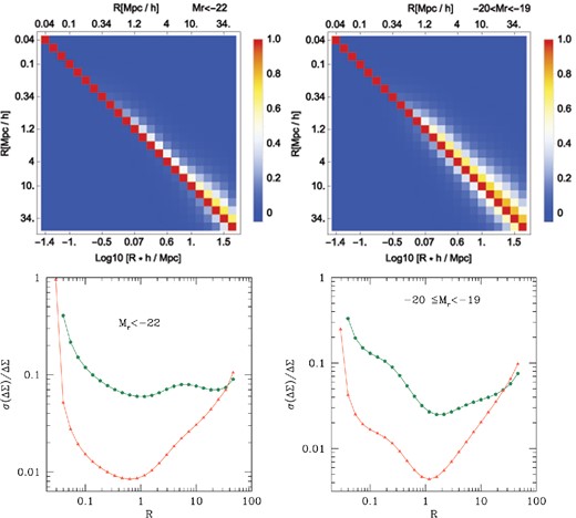
Theoretical estimates of the GGL correlation matrix and variance, illustrating the impact of shape noise for our brightest and faintest galaxy bins. Top panels: for each magnitude bin, the upper-right triangle corresponds to the level of noise from our MXXL measurements, while the bottom-left triangle has a shape noise similar to the SDSS measurements of Mandelbaum et al. (2013). Bottom panels: the noise-to-signal for the excess surface density. Green pentagons depict the prediction for the SDSS shape noise, and red triangles for the MXXL noise, i.e. the same as in Fig. 9.

Open in new tab Download slide

Download all slides

Month:	Total Views:
January 2017	2
February 2017	5
October 2017	3
November 2017	2
December 2017	5
January 2018	3
March 2018	1
April 2018	1
May 2018	2
June 2018	4
July 2018	4
August 2018	7
September 2018	7
October 2018	8
November 2018	5
December 2018	2
January 2019	8
February 2019	9
March 2019	7
April 2019	7
May 2019	8
June 2019	7
July 2019	11
August 2019	2
September 2019	4
October 2019	10
November 2019	7
December 2019	4
January 2020	5
February 2020	7
March 2020	7
April 2020	1
May 2020	2
June 2020	5
July 2020	2
August 2020	4
September 2020	4
October 2020	3
November 2020	3
December 2020	3
January 2021	4
February 2021	9
March 2021	8
April 2021	9
June 2021	7
July 2021	1
August 2021	3
September 2021	3
October 2021	2
November 2021	5
December 2021	1
January 2022	7
February 2022	6
March 2022	10
April 2022	19
May 2022	3
June 2022	3
July 2022	3
August 2022	9
September 2022	3
October 2022	6
November 2022	1
January 2023	3
February 2023	3
March 2023	5
April 2023	8
May 2023	2
June 2023	2
July 2023	6
August 2023	5
September 2023	2
October 2023	5
November 2023	6
December 2023	6
January 2024	5
February 2024	5
March 2024	3
April 2024	12
May 2024	8
June 2024	7
July 2024	3
September 2024	3
October 2024	15
November 2024	11
December 2024	5
January 2025	4
February 2025	4
March 2025	8
April 2025	9
May 2025	6

Article Contents

An exploration of galaxy–galaxy lensing and galaxy clustering in the Millennium-XXL simulation Free

Abstract

1 INTRODUCTION

2 THEORETICAL PREDICTIONS FOR THE GGL AND GC SIGNALS

2.1 Overview of required lensing ingredients

2.2 Estimator for the stacked tangential shear

2.3 The projected galaxy correlation function

3 SIGNAL COVARIANCE MATRICES

3.1 The covariance matrix of the stacked tangential shear estimator

3.2 The covariance matrix of the projected galaxy correlation function estimator

3.3 The cross-covariance of the stacked tangential shear and the projected galaxy correlation function estimators

4 THE MXXL SIMULATION

5 RESULTS I: CLUSTERING AND LENSING MEASUREMENTS IN MXXL

5.1 Methodology for estimating the projected correlation functions

5.2 Galaxy and matter correlation functions

5.3 Galaxy bias and cross-correlation coefficient

5.4 Comparison of the measured and theoretical projected galaxy correlation function

5.5 The stacked tangential shear of galaxies

6 RESULTS II: COVARIANCE MATRICES FROM THE MXXL

6.1 Covariance of the projected correlation function

6.2 Covariance of the stacked tangential shear

6.3 Cross-covariance of the projected correlation function and stacked tangential shear

6.4 Testing the jackknife method to estimate covariances

7 CONCLUSIONS

REFERENCES

APPENDIX A: DERIVATION OF THE AUTO- AND CROSS-COVARIANCE MATRICES

A1 Derivation of the covariance matrix of stacked tangential shear

A2 Derivation of the covariance matrix of the 3D galaxy correlation function

A3 Cross-covariance matrix of stacked tangential shear and the projected galaxy correlation function

APPENDIX B: GALAXY CATALOGUE COMPARISON

APPENDIX C: THE IMPACT OF SHAPE NOISE

Citations

Views

Altmetric

Email alerts

Astrophysics Data System

Citing articles via

Latest

Most Read

Most Cited

This Feature Is Available To Subscribers Only

An exploration of galaxy–galaxy lensing and galaxy clustering in the Millennium-XXL simulation