


Abstract
We investigate the internal structure and density profiles of haloes of mass 1010–1014 M⊙ in the Evolution and Assembly of Galaxies and their Environment (EAGLE) simulations. These follow the formation of galaxies in a Λ cold dark matter Universe and include a treatment of the baryon physics thought to be relevant. The EAGLE simulations reproduce the observed present-day galaxy stellar mass function, as well as many other properties of the galaxy population as a function of time. We find significant differences between the masses of haloes in the EAGLE simulations and in simulations that follow only the dark matter component. Nevertheless, haloes are well described by the Navarro–Frenk–White density profile at radii larger than ∼5 per cent of the virial radius but, closer to the centre, the presence of stars can produce cuspier profiles. Central enhancements in the total mass profile are most important in haloes of mass 1012–1013 M⊙, where the stellar fraction peaks. Over the radial range where they are well resolved, the resulting galaxy rotation curves are in very good agreement with observational data for galaxies with stellar mass M* < 5 × 10¹⁰ M⊙. We present an empirical fitting function that describes the total mass profiles and show that its parameters are strongly correlated with halo mass.
1 INTRODUCTION
The development of efficient computational techniques and the growing availability of computing power over the past three decades have made it possible to simulate the evolution of representative cosmological volumes at high enough resolution to follow the formation of cosmic structures over many orders of magnitude in mass.
The nearly scale-free behaviour induced by gravity applies only to haloes made entirely of DM. In practice, haloes of mass above ∼109 M⊙ participate in the process of galaxy formation. The cooling and dissipation of gas in these haloes introduces a characteristic scale that breaks self-similarity (White & Rees 1978; White & Frenk 1991) and the subsequent formation of stars can deepen the potential well and modify the structure of the halo in this region.
One of the early models of the effects of baryon collapse on the structure of a halo, making use of adiabatic invariants, concluded that haloes would become denser in their centres (Blumenthal et al. 1986). These simple models, however, were later shown not to match hydrodynamic simulations and led to a more general framework for calculating adiabatic contraction based on the average radial distribution of particles (Gnedin et al. 2004; Gustafsson, Fairbairn & Sommer-Larsen 2006). The parameters of this model, however, have been shown to depend on halo mass, redshift and on the details of the hydrodynamic simulation, making analytical descriptions of adiabatic contraction complex and uncertain (Duffy et al. 2010).
Baryons, however, can also produce the opposite effect and induce expansion rather than contraction of the halo. Using idealized hydrodynamic simulations, Navarro, Eke & Frenk (1996a) showed that the rapid expulsion of gas that had previously cooled to very high density near the centre of a halo could generate a central core. Subsequent work using cosmological simulations has confirmed and extended this result (e.g. Dehnen 2005; Read & Gilmore 2005; Mashchenko, Couchman & Wadsley 2006; Governato et al. 2010; Pontzen & Governato 2012; Martizzi, Teyssier & Moore 2013; Teyssier et al. 2013).
The structure of the inner halo is often used as a test of the Λ cold dark matter (ΛCDM) paradigm (e.g. Sand, Treu & Ellis 2002; Gilmore et al. 2007). Such tests, however, tend to compare observations of haloes which have galaxies within them with results from simulations of pure DM haloes (Newman et al. 2013). For the tests to be meaningful, accurate and reliable calculations of how baryons affect the structure of the haloes are essential. Such calculations are also of major importance for efforts to detect DM experimentally, either directly in the laboratory, or indirectly through the products of particle decay or annihilation.
Simulating the evolution of the visible components of the universe is a much more complex task than simulating the evolution of the DM because baryons undergo a variety of astrophysical processes many of which are relatively poorly understood. The resolution that is attainable even with the largest computers today is insufficient for an ab initio calculation of most of these processes which, as a result, need to be treated through parametrized ‘subgrid’ models added to the coupled hydrodynamical and gravitational evolution equations. These models describe the effects of radiative cooling, star formation, feedback from energy liberated during the evolution of stars and supermassive black holes (BHs) growing at the centres of galaxies. Simulations that include some or all of these processes have shown that significant changes can be induced in the total masses of haloes (Sawala et al. 2013, 2015; Cusworth et al. 2014; Velliscig et al. 2014; Vogelsberger et al. 2014) and in their inner structure (e.g. Gnedin et al. 2004; Pedrosa, Tissera & Scannapieco 2009; Duffy et al. 2010; Brook et al. 2012; Pontzen & Governato 2012; Di Cintio et al. 2014).
In this paper, we investigate how baryon physics modifies the structure of DM haloes in the Evolution and Assembly of Galaxies and their Environment (EAGLE) cosmological hydrodynamical simulations (Schaye et al. 2015). An important advantage of these simulations is that they give a good match to the stellar mass function and to the distribution of galaxy sizes over a large range of stellar masses [(108–1011.5) M⊙]. Furthermore, the relatively large volume of the reference EAGLE simulation provides a large statistical sample to derive the halo mass function in the mass range (109–1014) M⊙ and to investigate the radial density profiles of haloes more massive than 1011 M⊙.
This paper is organized as follows. In Section 2, we introduce the simulations and describe the selection of haloes. In Section 3, we focus on the change in the mass of haloes induced by baryon processes and the effect this has on the halo mass function. In Section 4, we analyse the radial density profile of the haloes and decompose them according to their different constituents. We fit the total matter profile with a universal formula that accounts for deviations from the NFW profile and show that the best-fitting parameters of these fits correlate with the mass of the halo. Our main results are summarized in Section 5. All our results are restricted to redshift z = 0 and all quantities are given in physical units (without factors of h).
2 THE SIMULATIONS
The simulations analysed in this paper were run as part of a Virgo Consortium project called the EAGLE (Schaye et al. 2015). The EAGLE project consists of simulations of ΛCDM cosmological volumes with sufficient size and resolution to model the formation and evolution of galaxies of a wide range of masses, and also include a counterpart set of DM-only simulations of these volumes. The galaxy formation simulations include the correct proportion of baryons and model gas hydrodynamics and radiative cooling. State-of-the-art subgrid models are used to follow star formation and feedback processes from both stars and active galactic nuclei (AGN). The parameters of the subgrid model have been calibrated to match certain observables as detailed in Schaye et al. (2015). In particular, the simulations reproduce the observed present day stellar mass function, galaxy sizes, and many other properties of galaxies and the intergalactic medium remarkably well. These simulations also show the correct trends with redshift of many galaxy properties (Schaye et al. 2015; Furlong et al. 2014).
The simulations were run using an extensively modified version of the code gadget-3 (Springel et al. 2008), which is essentially a more computationally efficient version of the public code gadget-2 described in detail by Springel (2005). gadget uses a tree-pm method to compute the gravitational forces between the N-body particles and implements the equations of hydrodynamics using smooth particle hydrodynamics (SPH; Monaghan 1992; Price 2010).
The EAGLE version of gadget-3 uses an SPH implementation called anarchy (Dalla Vecchia, in preparation), which is based on the general formalism described by Hopkins (2013), with improvements to the kernel functions (Dehnen & Aly 2012) and viscosity terms (Cullen & Dehnen 2010). This new implementation of SPH alleviates some of the problems associated with modelling contact discontinuities and fluid instabilities. As discussed by Dalla Vecchia (in preparation), the new formalism improves on the treatment of instabilities associated with cold flows and filaments and on the evolution of the entropy of hot gas in haloes. The timestep limiter of Durier & Dalla Vecchia (2012) is applied to ensure good energy conservation everywhere, including regions disturbed by violent feedback due to supernovae and AGN. The impact of this new hydrodynamics scheme on our galaxy formation model is discussed by Schaller et al. (in preparation).
The analysis in this paper focuses on two simulations: the Ref-L100N1504 simulation introduced by Schaye et al. (2015), which is the largest EAGLE simulation run to date, and its counterpart DM-only simulation, DM-L100N1504. To investigate smaller mass haloes and test for convergence in our results, we also analyse the higher resolution Recal-L025N0752 simulation (and its DM-only counterpart) in which some of the subgrid physics parameters were adjusted to ensure that this calculation also reproduces the observed galaxy stellar mass function, particularly at the low-mass end, as discussed by (Schaye et al. 2015). We will refer to the two simulations with baryon physics as ‘EAGLE’ simulations and to the ones involving only DM as ‘DMO’ simulations.
The main EAGLE simulation models a cubic volume of side-length 100 Mpc with 15043 gas and 15043 DM particles to redshift z = 0. A detailed description of the initial conditions is given in Schaye et al. (2015). Briefly, the starting redshift was z = 127; the initial displacements and velocities were calculated using second-order Lagrangian perturbation theory with the method of Jenkins (2010); the linear phases were taken from the public multiscale Gaussian white noise field, Panphasia (Jenkins 2013); the cosmological parameters were set to the best-fitting ΛCDM values given by the Planck-1 data (Planck Collaboration XVI 2014): |$\left[\Omega _{\rm {m}}, \Omega _{\rm {b}}, \Omega _\Lambda ,h,\sigma _8,n_s\right] = \left[0.307, 0.04825, 0.693, 0.6777, 0.8288, 0.9611\right]$|; and the primordial mass fraction of He was set to 0.248. These choices lead to a DM particle mass of 9.70 × 10⁶ M⊙ and an initial gas particle mass of 1.81 × 10⁶ M⊙. We use a comoving softening of 2.66 kpc at early times, which freezes at a maximum physical value of 700 pc at z = 2.8. The Recal-L025N0752 simulation follows 7523 gas and 7523 DM particles in a 25 Mpc volume assuming the same cosmological parameters. This implies a DM particle mass of 1.21 × 10⁶ M⊙ and an initial gas mass of 2.26 × 10⁵ M⊙. The softening is 1.33 kpc initially and reaches a maximum physical size of 350 pc at z = 0.
The DMO simulations, DM-L100N1504 and DM-L025N0752, follow exactly the same volume as EAGLE, but with only 15043 and 7523 collisionless DM particles, each of mass 1.15 × 10⁷ M⊙ and 1.44 × 10⁶ M⊙, respectively. All other cosmological and numerical parameters are the same as in the EAGLE simulation.
2.1 Baryonic physics
The baryon physics in our simulation correspond to the Ref EAGLE model. The model, fully described in Schaye et al. (2015), is summarized here for completeness.
Star formation is implemented following Schaye & Dalla Vecchia (2008). A polytropic equation of state, P ∝ ρ4/3, sets a lower limit to the gas pressure. The star formation rate per unit mass of these particles is computed using the gas pressure using an analytical formula designed to reproduce the observed Kennicutt–Schmidt law (Kennicutt 1998) in disc galaxies (Schaye & Dalla Vecchia 2008). Gas particles are converted into stars stochastically. The threshold in hydrogen density required to form stars is metallicity dependent with lower metallicity gas having a higher threshold, thus capturing the metallicity dependence of the |$\rm {HI}{\rm -}\rm {H}_2$| phase transition (Schaye 2004).
The stellar initial mass function (IMF) is assumed to be that of Chabrier (2003) in the range 0.1–100 M⊙ with each particle representing a single age stellar population. After 3 × 10⁷ yr, all stars with an initial mass above 6 M⊙ are assumed to explode as supernovae. The energy from these explosions is transferred as heat to the surrounding gas. The temperature of an appropriate amount of surrounding gas is raised instantly by 107.5 K. This heating is implemented stochastically on one or more gas particles in the neighbourhood of the explosion site (Dalla Vecchia & Schaye 2012). This gas, once heated, remains coupled in a hydrodynamic sense with its SPH neighbours in the interstellar medium (ISM), and therefore exerts a form of feedback locally that can affect future star formation and radiative cooling.
Besides energy from star formation, the star particles also release metals into the ISM through three evolutionary channels: Type Ia supernovae, winds, and supernovae from massive stars, and AGB stars using the method discussed in Wiersma et al. (2009). The yields for each process are taken from Portinari, Chiosi & Bressan (1998), Marigo (2001) and Thielemann et al. (2003). Following Wiersma, Schaye & Smith (2009), the abundances of the eleven elements that dominate the cooling rates are tracked. These are used to compute element-by-element-dependent cooling rates in the presence of the cosmic microwave background and the ultraviolet and X-ray backgrounds from galaxies and quasars according to the model of Haardt & Madau (2001).
Feedback due to AGN activity is implemented in a similar way to the feedback from star formation described above. The fraction of the accreted rest mass energy liberated by accretion is ϵr = 0.1, and the heating efficiency of this liberated energy (i.e. the fraction of the energy that couples to the gas phase) is ϵf = 0.15. Gas particles receiving AGN feedback energy are chosen stochastically and their temperature is raised by 108.5 K.
These models of supernova and AGN feedback are extensions of the models developed for the Virgo Consortium projects OWLS (Schaye et al. 2010) and GIMIC (Crain et al. 2009). The values of the parameters were constrained by matching key observables of the galaxy population including the observed z ≈ 0 galaxy stellar mass function, galaxy sizes and the relation between BH and stellar mass (Crain et al. 2015).
2.2 Halo definition and selection
2.3 Matching haloes between the two simulations
The EAGLE and DMO simulations start from identical Gaussian density fluctuations. Even at z = 0 it is possible, in most cases, to identify matches between haloes in the two simulations. These matched haloes are comprised of matter that originates from the same spatial locations at high redshift in the two simulations. In practice, these identifications are made by matching the particle IDs in the two simulations, as the values of the IDs encode the Lagrangian coordinates of the particles in the same way in both simulations.
For every FOF group in the EAGLE simulation, we select the 50 most bound DM particles. We then locate those particles in the DMO simulation. If more than half of them are found in a single FOF group in the DMO simulation, we make a link between those two haloes. We then repeat the procedure by looping over FOF groups in the DMO simulation and looking for the position of their counterparts in the EAGLE simulation. More than 95 per cent of the haloes with M200 > 2 × 10¹⁰ M⊙ can be matched bijectively, with the fraction reaching unity for haloes above 7 × 10¹⁰ M⊙ in the L100N1504 volumes. Similarly, 95 per cent of the haloes with M200 > 3 × 10⁹ can be matched bijectively in the L025N0752 volumes.
3 HALO MASSES AND CONTENT
Previous work comparing the masses of haloes in cosmological galaxy formation simulations with matched haloes in counterpart DM-only simulations have found strong effects for all but the most massive haloes (e.g. Cui et al. 2012; Sawala et al. 2013). Sawala et al. (2013) found that baryonic effects can reduce the masses of haloes by up to 25 per cent for halo masses (in the DM only simulation) below 1013 M⊙. (They did not include AGN feedback in their simulation.) A similar trend was observed at even higher masses by Martizzi et al. (2013), Velliscig et al. (2014), Cui, Borgani & Murante (2014), and Cusworth et al. (2014) using a variety of subgrid models for star formation and stellar and AGN feedback. All these authors stress that their results depend on the details of the subgrid implementation used. This is most clearly shown in Velliscig et al. (2014), where the amplitude of this shift in mass is shown explicitly to depend on the subgrid AGN feedback heating temperature, for example. Hence, it is important to use simulations that have been calibrated to reproduce the observed stellar mass function.
In this section, we find that similar differences to those seen before occur between halo masses in the EAGLE and DMO models. These differences are of particular interest because EAGLE reproduces well a range of low-redshift observables of the galaxy population such as masses, sizes, and star formation rates (Schaye et al. 2015), although the properties of clusters of galaxies are not reproduced as well as in the COSMO-OWLS simulation (Le Brun et al. 2014) analysed by Velliscig et al. (2014).
3.1 The effect of baryon physics on the total halo mass
In this section, we compare the masses of haloes in the EAGLE and DMO simulations combining our simulations at two different resolutions. To minimize any possible biases due to incomplete matching between the simulations, we only consider haloes above 3 × 10⁹ M⊙ (in DMO), since these can be matched bijectively to their counterparts in more than 95 per cent of cases.
Fig. 1 shows the ratio of M200 for matched haloes in the EAGLE and DMO simulations as a function of M200 in the DMO simulation. The black filled circles correspond to the geometric mean of the ratios in each logarithmically spaced mass bin. The choice of a geometric mean is motivated simply by the fact that its reciprocal is the geometric mean of |$M_{200}^{\rm {DMO}}/M_{200}^{\rm {EAGLE}}$|, which is also a quantity of interest.
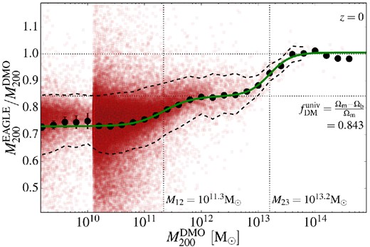
The ratio of the masses of the matched haloes in the EAGLE and DMO simulations. The red squares show values for individual haloes and the black filled circles values binned by DMO halo mass. Haloes with |$M_{200}^{\rm DMO} < 10^{10.1}\,{\rm {M}_{\odot }}$| are extracted  from the higher resolution, L025N0752, simulation. The binned points are the geometric average of the individual ratios with the error bars at |$M_{200}^{\rm DMO} < 10^{10.1}\,{\rm {M}_{\odot }}$| indicating the uncertainty arising from the low number of haloes in the high-resolution simulation. The black dashed lines placed above and below the black points show the geometrical 1σ scatter for each bin. The lower horizontal grey dotted line indicates the universal DM fraction fDM = 1 − fb = (Ωm − Ωb)/Ωm = 0.843. The upper dotted line marks unity. The green solid line is the function of equation (13) fitted to the binned ratios. The vertical dotted lines mark the values of the fitting parameters M12 and M23.
The haloes in EAGLE are typically lighter than their DMO counterparts. There appear to be three distinct regimes in Fig. 1. At the low mass end, M200 < 5 × 10¹⁰ M⊙, |$M_{200}^{\rm {EAGLE}}/M_{200}^{\rm {DMO}}$| drops to ∼0.72. This is less than one minus the universal baryon fraction, fDM, so not only have the baryons been removed but the DM has also been disturbed. The reduction in mass due to the loss of baryons lowers the value of R200 and thus the value of M200. However, this reduction in radius is not the sole cause for the reduction in halo mass: the amount of mass within a fixed physical radius is actually lower in the simulation with baryons because the loss of baryons, which occurs early on, reduces the growth rate of the halo (Sawala et al. 2013). At higher masses, stellar feedback becomes less effective, but AGN feedback can still expel baryons and the ratio rises to a plateau of ∼0.85 between |$M_{200}^{\rm {DMO}}=10^{12}$| and 5 × 10¹² M⊙. Finally, for the most massive haloes (M200 > 1014 M⊙) not even AGN feedback can eject significant amounts of baryons from the haloes and the mass ratio asymptotes to unity.
It is quite clear, however, from Fig. 1 that a single sigmoid function does not reproduce the behaviour we observe particularly well: the ratio shows three, not two, distinct plateaux. The simulations used by Sawala et al. (2013) did not include AGN feedback and so did not show the change in mass arising from this form of feedback. In contrast, the simulations used by Velliscig et al. (2014) did not have sufficient numerical resolution to see the asymptotic low-mass behaviour determined by stellar feedback.
The green curve in Fig. 1 shows the best-fitting curve to the black binned data points. The fit was obtained by a least-squares minimization for all seven parameters assuming Poisson uncertainties for each mass bin. Adopting a constant error instead gives very similar values for all parameters. The values of the two transition masses, M12 and M23, are shown as vertical dotted lines in Fig. 1. The best-fitting parameters are given in Table 1. Note that the value of r3 is, as expected, very close to unity.
| Parameter | Value | 1σ fit uncertainty |
|---|---|---|
| r1 | 0.7309 | ±0.0014 |
| r2 | 0.8432 | ±0.0084 |
| r3 | 1.0057 | ±0.0024 |
| log10(M12/M⊙ | 11.33 | ±0.003 |
| log10(M23/M⊙ | 13.19 | ±0.029 |
| t12 | 1.721 | ±0.045 |
| t23 | 2.377 | ±0.18 |
| Parameter | Value | 1σ fit uncertainty |
|---|---|---|
| r1 | 0.7309 | ±0.0014 |
| r2 | 0.8432 | ±0.0084 |
| r3 | 1.0057 | ±0.0024 |
| log10(M12/M⊙ | 11.33 | ±0.003 |
| log10(M23/M⊙ | 13.19 | ±0.029 |
| t12 | 1.721 | ±0.045 |
| t23 | 2.377 | ±0.18 |
| Parameter | Value | 1σ fit uncertainty |
|---|---|---|
| r1 | 0.7309 | ±0.0014 |
| r2 | 0.8432 | ±0.0084 |
| r3 | 1.0057 | ±0.0024 |
| log10(M12/M⊙ | 11.33 | ±0.003 |
| log10(M23/M⊙ | 13.19 | ±0.029 |
| t12 | 1.721 | ±0.045 |
| t23 | 2.377 | ±0.18 |
| Parameter | Value | 1σ fit uncertainty |
|---|---|---|
| r1 | 0.7309 | ±0.0014 |
| r2 | 0.8432 | ±0.0084 |
| r3 | 1.0057 | ±0.0024 |
| log10(M12/M⊙ | 11.33 | ±0.003 |
| log10(M23/M⊙ | 13.19 | ±0.029 |
| t12 | 1.721 | ±0.045 |
| t23 | 2.377 | ±0.18 |
The value of the first transition mass, M12 = 1011.35 M⊙, is similar to that reported by Sawala et al. (2013) who found Mt = 1011.6 M⊙ for the GIMIC simulations. The second transition, M32 = 1013.2 M⊙, is located well below the range of values found by Velliscig et al. (2014) (1013.7 –1014.25 M⊙). However, as Schaye et al. (2015) have shown the AGN feedback in the few rich clusters formed in the EAGLE volume may not be strong enough, as evidenced by the fact that this simulation overestimates the gas fractions in clusters, whereas the 400 Mpc h− 1 COSMO-OWLS simulation used by Velliscig et al. (2014) reproduces these observations (Le Brun et al. 2014).
A simulation with stronger AGN feedback, EAGLE-AGNdT9, which gives a better match to the group gas fractions and X-ray luminosities than EAGLE, was discussed by Schaye et al. (2015). Applying the same halo matching procedure to this simulation and its collisionless DM-only counterpart, we obtain slightly different values for the best-fitting parameters of equation (13). The difference is mainly in the parameters, M23 and t23, which describe the high-mass end of the double-sigmoid function. In this model, the transition occurs at log 10(M23/M⊙) = 13.55 ± 0.09, closer to the values found by Velliscig et al. (2014). The width of the transition, however, is poorly constrained, t23 = 3.0 ± 12.7, due to the small number of haloes (only eight with M200, DMO > 2 × 10¹³ M⊙) in this simulation which had only an eighth the volume of the reference simulation.
3.2 The halo mass function
The effect of baryons on the halo mass function can be seen in Fig. 2. The red and green lines in the top panel show the mass functions in the EAGLE and DMO simulations. The ratio of the two functions (bottom panel) shows an almost constant shift over most of the plotted mass range, M200/ M⊙ = 109–1013, as expected from Fig. 1. The relatively small volume of the EAGLE simulation does not sample the knee of the halo mass function well, but extrapolating the fit to the mass ratios of equation (13) to higher masses, together with results from previous studies (Martizzi et al. 2013; Cusworth et al. 2014; Velliscig et al. 2014), suggests that the differences vanish for the most massive objects. Studies that rely on galaxy clusters to infer cosmological parameters will need to take account of the effects of the baryons, particularly for clusters of mass M200 ≲ 1014 M⊙.
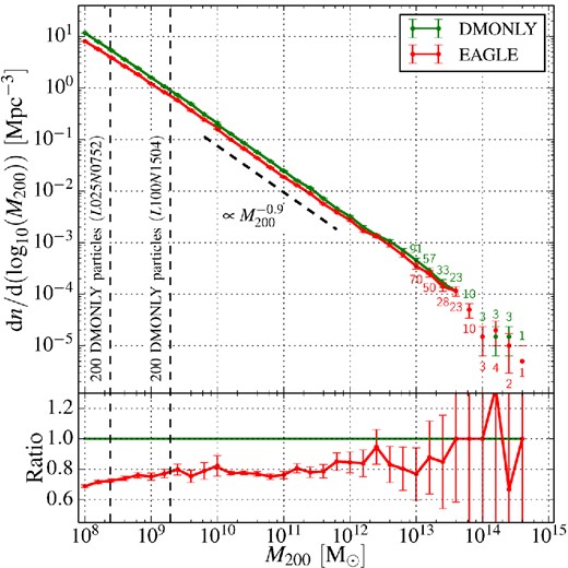
Top panel: the abundance of haloes at z = 0 as a function of the mass, M200, in the EAGLE (red curve, lower line) and DMO (green curve, upper line) simulations. The high-resolution volume is used for |$M_{200}^{\rm DMO} < 10^{10.1}\,{\rm {M}_{\odot }}$|. The resolution limits for both simulations are indicated by the vertical dashed lines on the left, and the number of haloes in sparsely populated bins is given above the Poisson error bars. Bottom panel: the ratio of the mass functions in the EAGLE and DMO simulations.
3.3 Baryonic and stellar fractions in the EAGLE simulation
We have shown in the previous subsection that for all but the most massive examples, halo masses are systematically lower when baryonic processes are included. In this subsection, we examine the baryonic content of haloes in the EAGLE simulation. We restrict our analysis to the L100N1504 volume.
Fig. 3 shows the mass fractions of baryons and stars within R200 as a function of the halo mass, M200, in the EAGLE simulation. The baryon fraction increases with halo mass and approaches the universal mean value, |$f_{\rm b}^{\rm {univ}} \equiv \Omega _{\rm {b}}/\Omega _{\rm {m}}$|, for cluster mass haloes. The gas is the most important baryonic component in terms of mass over the entire halo mass range. At a much lower amplitude everywhere, the stellar mass fraction peaks around a halo mass scale of 2 × 10¹² M⊙ where star formation is at its least inefficient.
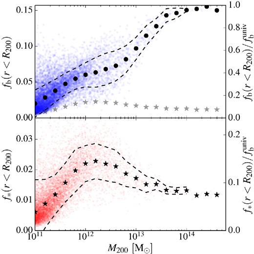
Baryon fraction, fb = Mb/M200 (top panel), and stellar fraction, f* = M★/M200 (bottom panel), within R200 as a function of M200. The right-hand axis gives the fractions in units of the universal mean value, |$f_{\rm b}^{\rm {univ}}=0.157$|. The solid circles in the top panel and the stars in the bottom panel show the mean value of the fractions binned by mass. The dashed lines above and below these symbols show the rms width of each bin with more than three objects. The stellar fractions are reproduced as grey stars in the top panel.
The baryon fractions are much lower than the universal value for all but the most massive haloes. For Milky Way-sized haloes, we find |$f_{\rm b} / f_{\rm b}^{\rm {univ}} \approx 0.35$|. It is only for group and cluster sized haloes, whose deeper gravitational potentials are able to retain most of the baryons even in the presence of powerful AGN, that the baryon fraction is close to |$f_{\rm b}^{\rm {univ}}$|. The baryon fractions of the haloes extracted from the EAGLE-AGNdT9 model (which provides a better match to X-ray luminosities; Schaye et al. 2015) are presented in Appendix A1.
The stellar mass fraction is never more than a few per cent. At the peak, around M200 ≈ 2 × 10¹² M⊙, it reaches a value of ∼0.023. Multiplying the stellar fraction by the halo mass function leads to an approximate stellar mass function, which is close to the actual one (published in Schaye et al. 2015), after a fixed aperture correction is applied to mimic observational measurements. As may be seen in both panels, there is significant scatter in the baryonic and stellar fractions, with variations of a factor of a few possible for individual haloes.
While the baryonic and stellar fractions are low within R200, they are much higher in the inner regions of haloes as shown in Fig. 4, where these fractions are now plotted within 0.05R200, a scale commensurate with the sizes of galaxies both in EAGLE and in the real universe. Within this radius, the fractions rise above the cosmic mean for haloes in the mass range 5 × 10¹¹ M⊙ < M200 < 2 × 10¹³ M⊙. The central parts of these haloes are strongly dominated by the baryons. In agreement with observations of the nearby universe, the most important contribution to the mass on these scales is from stars rather than gas. Another notable feature is that the most massive haloes are baryon poor in their central regions, reflecting the regulation by AGN feedback.
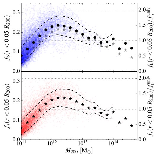
Same as Fig. 3 but for the mass contained within 5 per cent of R200. Note the different scale on the ordinate axis. The dotted horizontal lines mark one and two times the universal baryon fraction.
4 HALO PROFILES
In this section, we explore the effects of baryons on halo profiles restricting the analysis to haloes with more than 5000 particles within Rvir, which corresponds to a halo mass of about 5 × 10¹⁰ M⊙ in the L100N1504 simulation and 6 × 10⁹ M⊙ in the L050N0752 simulation. The stellar masses found in the EAGLE simulation for haloes of this mass are consistent with observational expectations based on abundance matching (Schaye et al. 2015). Haloes smaller than this typically have fewer than the hundred star particles, which Schaye et al. (2015) showed to be a necessary criterion for many applications. This limit of 5000 in the number of particles is intermediate between those used in other studies. It is similar to the number adopted by Ludlow et al. (2013) and lower than the number adopted by Neto et al. (2007) and Duffy et al. (2008, 2010, 10 000 particles), but higher than the number adopted by Gao et al. (2008), Dutton & Macciò (2014, 3000 particles), or Macciò et al. (2007, 250 particles). There are 22 867 haloes with at least 5000 particles in the Ref-L100N1504 EAGLE simulation and 2460 in the Recal-L025N0752 simulation.
We define relaxed haloes as those where the separation between the centre of the potential and the centre of mass is less than 0.07Rvir, as proposed by Macciò et al. (2007). Neto et al. (2007) used this criterion, and also imposed limits on the substructure abundance and virial ratio. Neto et al. (2007) found that the first criterion was responsible for rejecting the vast majority of unrelaxed haloes. Their next most discriminating criterion was the amount of mass in substructures. In common with Gao et al. (2008), here we use stacked profiles. Hence, individual substructures, which can be important when fitting individual haloes, have a smaller effect on the average profile. We therefore do not use a substructure criterion to reject haloes. Our relaxed sample includes 13426 haloes in the L100N1504 simulation and 1590 in the L025N0752 simulation. We construct the stacked haloes by coadding haloes in a set of contiguous bins of width Δlog10(M200) = 0.2.
The density and mass profiles of each halo and of the stacked haloes are obtained using the procedure described by Neto et al. (2007). We define a set of concentric contiguous logarithmically spaced spherical shells of width Δlog10(r) = 0.078, with the outermost bin touching the virial radius, Rvir. The sum of the masses of the particles in each bin is then computed for each component (DM, gas, stars, BHs) and the density is obtained by dividing each sum by the volume of the shell.
4.1 Resolution and convergence considerations
While this criterion could be applied to the DMO simulation, the situation for the EAGLE simulation is more complex since, as discussed by Schaye et al. (2015), the concept of numerical convergence for the adopted subgrid model is itself ill defined. One option would be simply to apply the P03 criterion, which is appropriate for the DMO simulation, to both simulations. Alternatively, we could apply the criterion to the DM component of the haloes in the baryon simulation or to all the collisionless species (stars, DM, and BHs). Neither of these options is fully satisfactory but, in practice, they lead to similar estimates for RP03. For the smallest haloes of the L100N1504 simulation considered in this section, we find RP03 ≈ 5.1 kpc whereas for the largest clusters we obtain RP03 ≈ 3.5 kpc.
The original P03 criterion ensures that the mean density internal to the convergence radius, |$\bar{\rho }= 3M(r<R_{P03}) / 4\pi R_{P03}^3$|, is within 10 per cent of the converged value obtained in a simulation of much higher resolution. As the magnitude of the differences between the EAGLE and DMO profiles that we see are significantly larger than 10 per cent typically, we can relax the P03 criterion somewhat. Reanalysing their data, we set the coefficient on the left-hand side of equation (15) to 0.33, which ensures a converged value of the mean interior density at the 20 per cent level. With this definition, our minimal convergence radius rc takes values between 4 and 2.9 kpc for haloes with M200 ∼ 1011 M⊙ up to M200 ∼ 1014 M⊙. Similarly, in the L025N0752 simulation our modified criterion gives rc ≈ 1.8 kpc. Note that despite adopting a less conservative criterion than P03, the values of rc are always greater than the Plummer equivalent softening length where the force law becomes Newtonian, 2.8ϵ = 0.7 kpc in the L100N1504 simulation and 0.35 kpc in L025N0752 simulation.
The validity of our adopted convergence criterion can be tested directly by comparing results from our simulations at two different resolutions. Specifically, we compare our two simulations of (25 Mpc)3 volumes, L025N0752, and L025N0376 which has the same initial phases as L025N0752 but the resolution of the reference, L100N1504, simulation. In the language of Schaye et al. (2015), this is a weak convergence test since the parameters of the subgrid models have been recalibrated when increasing the resolution.
Fig. 5 shows the stacked profiles of the 44 relaxed haloes of mass 1011 M⊙ present in both the L025N0376 and L025N0752 simulations. This mass bin contains enough haloes for the stacks not to be dominated by Poisson noise and the haloes are large enough to contain more than 5000 particles in the lower resolution simulation. The three panels show density, contained mass, and circular velocity profiles respectively, using symbols for the default resolution and lines for the higher resolution simulation. As may be seen, the stacked DM and total matter profiles are very well converged over most of the radial range, both in terms of the integral quantities, M(r) and Vc(r), and in terms of the differential quantity, ρ(r). The dashed and dotted vertical lines show the convergence radius, rc, for the default and high-resolution simulations, respectively, computed following the procedure described above.
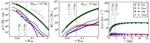
From left to right: the density, mass and circular velocity profiles of a stack of the 44 relaxed haloes of mass 1011 M⊙ at z = 0 that are present in both the L025N0752 simulation (lines) and the L025N0376 simulation (symbols). Profiles of total matter (green), DM (black), gas (blue) and the stellar component (red) are shown for both resolutions. The vertical dashed and dotted lines show the resolution limits, rc, derived from our modified P03 criterion for the L025N0376 and L025N0752 simulations, respectively; data point are only shown at radii larger than the Plummer equivalent force softening. The DM, total matter, and stellar profiles are well converged even at radii smaller than rc, indicating that this convergence criterion is very conservative when relaxed haloes in a narrow mass range are averaged together. Convergence is much poorer for the subdominant gas distribution at large radii.
The DM and total matter profiles converge well down to much smaller radii than rc implying that this limit is very conservative. This is a consequence of comparing stacked rather than individual haloes since the stacks tend to average deviations arising from the additional mass scales represented in the high-resolution simulation. We conclude from this analysis that the total matter and DM profiles of stacked haloes are well converged in our simulations and that we can draw robust conclusions about their properties for r > rc in both the L100N1504 and L025N0752 simulations.
The gas profiles in these simulations display a much poorer level of convergence. The disagreement between the two simulations increases at radii larger than r > rc. However, since the mass in gas is negligible at all radii and at all halo masses, the poor convergence of the gas profiles does not affect our conclusions regarding the dark and total matter profiles. We defer the question of the convergence of gaseous profiles to future studies and simulations.
4.2 Stacked halo density and cumulative mass of relaxed haloes
Having established a robust convergence criterion for stacked haloes, we now analyse their profiles extracting haloes of mass M200 ≥ 1011 M⊙ from the L100N1504 simulation and haloes of mass 1010 M⊙ ≤ M200 ≤ 1011 M⊙ from the L025N0376 simulation.
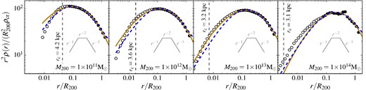
Fig. 6 shows the stacked profiles for five different halo mass bins. The left-hand column shows that the DM is the dominant component of the density of haloes of all masses outside about 1 per cent of R200. Inside this radius, the stellar component begins to contribute and even dominate in the case of haloes with mass ≳1012 M⊙. Considering only the baryonic matter, the inner radii are dominated by stars, but gas dominates outside of ∼0.1R200, as we already saw in Fig. 3. In haloes of Milky Way size (M200 ∼ 1012 M⊙), the density profile of the gas is roughly isothermal with ρ(r) ∝ r−2. The stars exhibit a steep profile, ρ(r) ∝ r−3 − r−4, in the region where this is resolved (r > rc). The resolution of our simulations is not sufficient to enable the discussion of the stellar profile in the central part of the galaxies, within ∼ 3 kpc of the centre of potential.
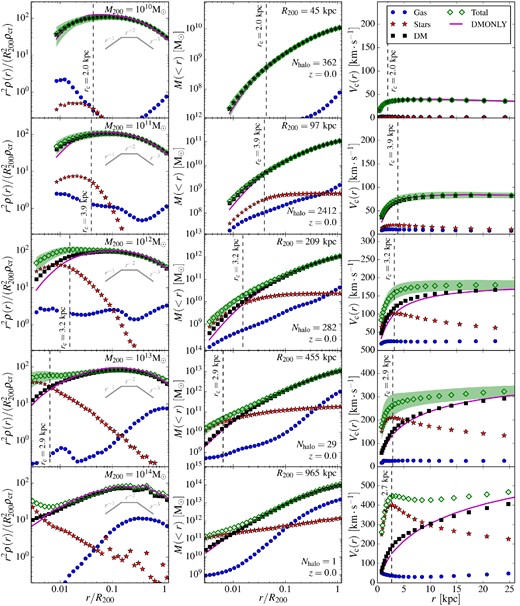
From left to right: the density, mass, and circular velocity profiles for stacks of relaxed haloes in different mass bins at z = 0. From top to bottom: bins centred on M200 ≈ 1010, 1011, 1012, 1013, and 1014 M⊙. Profiles of the total matter (green diamonds), DM (black squares), gas (blue circles) and stellar component (red stars) are shown for the haloes extracted from the EAGLE simulation. Profiles extracted from haloes of similar mass in the DMO simulation are shown with a magenta solid line on all panels. The rms scatter of the total profile is shown as a green shaded region. The vertical dashed line shows the (conservative) resolution limit, rc, introduced in the previous subsection; data are only shown at radii larger than the force softening. The number of haloes in each mass bin is indicated in the middle panel of each row. The density profiles have been multiplied by r2 and normalized to reduce the dynamic range of the plot and to enable easier comparisons between different halo masses. Note that following the analysis of Section 3.1, matched haloes are not guaranteed to fall into the same mass bin. The oscillations seen in the profiles of the two highest mass bins, which have only a few examples, are due to the object-to-object scatter and the presence of substructures.
The shape of the DM profiles in the EAGLE simulation is typically very close to those obtained in the DMO simulation. The profiles depart from the DMO shape in haloes with M200 ≳ 1012 M⊙, where the slope in the inner regions (below 0.1R200) is slightly steeper. This indicates that some contraction of the DM has taken place, presumably induced by the presence of baryons in the central region.
The total density profiles of the EAGLE haloes also closely resemble those of the DMO simulation. This follows because the DM dominates over the baryons at almost all radii. In haloes with a significant stellar fraction, the total profile is dominated by the stars within ∼0.01R200. This creates a total inner profile that is steeper than in the DMO simulations. The stellar contribution is dominant only in the first few kiloparsecs almost independently of the halo mass. Given that DMO haloes have profiles similar to an NFW profile, this implies that the total profile will be closer to an NFW for more massive haloes because the stars will only be important inside a smaller fraction of the virial radius. This is most clearly seen in the 1014 M⊙ halo where the profile is dominated by the DM and follows the NFW form down to 0.01R200. Similarly, in the smallest haloes, M200 ≈ 1010 M⊙, the baryon content is so low that the total matter profile behaves almost exactly like the DM profile and is hence in very good agreement with DM-only simulations.
It is also interesting to note the absence in our simulations of DM cores of size 0.5-2 kpc such as have been claimed in simulations of individual haloes of various masses, assuming different subgrid models and, in some cases, different techniques for solving the hydrodynamical equations (e.g. Navarro et al. 1996a; Read & Gilmore 2005; Mashchenko et al. 2006; Pontzen & Governato 2012; Martizzi et al. 2013; Teyssier et al. 2013; Arraki et al. 2014; Pontzen & Governato 2014; Murante et al. 2015; Oñorbe et al. 2015; Trujillo-Gomez et al. 2015), even though such cores would have been resolved in our highest resolution simulations. As first shown by Navarro et al. (1996a), density cores can be generated by explosive events in the central regions of haloes when gas has become self-gravitating. Our simulations include violent feedback processes but these are not strong enough to generate a core or even a systematic flattening of the inner DM profile on resolved scales. We cannot, of course, rule out the possibility that the central profile could be modified even with our assumed subgrid model in higher resolution simulations.
4.3 Halo circular velocities
The right-hand column of Fig. 6 shows the rotation curves. Those for Milky Way mass haloes display a flat profile at radii greater than 10 kpc as observed in our galaxy and others (e.g. Reyes et al. 2011). The dominant contribution of the DM is clearly seen here. The stellar component affects only the first few kiloparsecs of the rotation curve. The rotation curves of haloes with a significant (>0.01) stellar fraction (i.e. haloes with M200 > 3 × 10¹¹ M⊙) have a higher amplitude than the corresponding DMO stacked curves at small radii r ≲ 10 kpc. The combination of the stellar component and contraction of the inner DM halo leads to a maximum rotation speed that is ≈30 per cent higher in the EAGLE simulation compared to that in DMO.
To assess whether the circular velocity profiles for the galaxies in the EAGLE simulation are realistic, we compare them to a sample of observed disc galaxies. We use the data from Reyes et al. (2011), who observed a sample of 189 spiral galaxies and used Hα lines to measure the circular speeds. From their SDSS r-band magnitudes and g − r colours, we derive the stellar masses of their galaxies using the M*/L scaling relation of Bell et al. (2003). We apply a − 0.1 dex correction to adjust these stellar mass estimates from their assumed ‘diet Salpeter’ IMF to our adopted Chabrier (2003) IMF, and apply the correction from Dutton et al. (2011) to convert our masses to the MPA/JHU definitions (See McCarthy et al. 2012 for the details.).
In Fig. 7, we show the rotation curves of our sample of relaxed haloes binned by the stellar mass contained within an aperture of 30 kpc, as used by Schaye et al. (2015) who already compared the predicted maximum circular velocities to observations. The simulated galaxies match the observations exceptionally well, both in terms of the shape and the normalization of the curves. For all mass bins up to M* < 1011 M⊙, the EAGLE galaxies lie well within the scatter in the data. Both the shape and the amplitude of the rotation curves are reproduced in the simulation. The scatter appears to be larger in the real than in the simulated population, particularly in the range 10.5 < log 10M*/M⊙ < 10.75 (lower left panel), but the outliers in the data might affected by systematic errors (Reyes et al. 2011) arising, for instance, from the exact position of the slit used to measure spectral features or from orientation uncertainties.
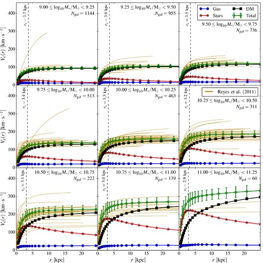
Simulated circular velocity curves and observed spiral galaxy rotation curves in different stellar mass bins. The green diamonds with error bars correspond to the total circular velocity and the rms scatter around the mean. The black squares, red stars, and blue circles represent the mean contributions of DM, star, and gas particles, respectively. The dashed vertical line is the conservative resolution limit, rc. The background brown curves are the best-fitting Hα rotation curves extracted from Reyes et al. (2011). We plot their data up to their i-band-measured isophotal R80 radii.
The rotation curves for the highest stellar mass bin in the simulation, M* > 1011 M⊙, show a clear discrepancy with the data. Although the general shape of the curves is still consistent, the normalization is too high. Part of this discrepancy might be due to the selection of objects entering into this mass bin. The data refer to spiral galaxies, whereas no selection besides stellar mass has been applied to the sample of simulated haloes. This highest mass bin is dominated by elliptical objects in EAGLE. Selecting spiral-like objects (in a larger simulation) may well change the results at these high stellar masses. A more careful measurement of the rotation velocities in the simulations in a way that is closer to observational estimates (e.g. by performing mock observations of stellar emission lines) might also reduce the discrepancies. We defer this, more careful, comparison to future work.
At all masses beyond the convergence radius, the dominant contribution to the rotation curve comes from the DM. For the highest mass bins, the stellar contribution is very important near the centre and this is crucial in making the galaxy rotation curves relatively flat. As already seen in the previous figure, the contribution of gas is negligible.
4.4 An empirical universal density profile
It is well known that the density profiles of relaxed haloes extracted from DM-only simulations are well fit by the NFW profile (equation 1) at all redshifts down to a few per cent of the virial radius (Navarro et al. 1997, 2004; Bullock et al. 2001; Eke et al. 2001; Shaw et al. 2006; Macciò et al. 2007; Neto et al. 2007; Duffy et al. 2008; Ludlow et al. 2013; Dutton & Macciò 2014). The total matter profiles shown in Fig. 6 for the EAGLE simulation follow the NFW prediction in the outer parts, but the inner profile is significantly steeper than the NFW form, which has an inner slope (ρ(r → 0) = r−η with η ≈ 1). The deviations from an NFW profile can be quite large on small scales.
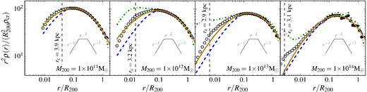
To show this, we fit the total mass profiles using the fitting procedure defined by Neto et al. (2007). We fit an NFW profile to the stacked profiles over the radial range [0.05, 1]Rvir, shown, respectively, as blue dashed curves and filled circles in Fig. 8. This choice of minimum radius is larger than the conservative convergence radius given by version of the P03 criterion that we adopted in the previous section. As described in Section 4.2, the bins are spherical and spaced logarithmically in radius.
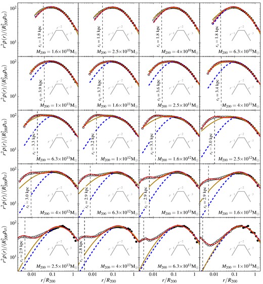
Stacked density profiles of the total mass normalized by the average R200 radius and scaled by r2 for haloes of different masses. The filled circles are the data points used to fit an NFW profile following Neto et al. (2007), i.e. radial bins above data points below it are shown using fainter symbols. The blue dashed lines correspond to the NFW fit to the filled circles, while the brown lines correspond to an Einasto profile fit to all radial bins down to the convergence radius, rc. The red solid line is the best-fitting profile given by equation (19), which includes an NFW contribution for the outer parts of the haloes and an additional contribution around the centre to model the baryons. The best-fitting parameters for each mass bins are given in Table 2.
The best-fitting profile for each stacked halo mass bin is shown in Fig. 8 as a blue dashed line. The NFW profile is a very good fit to the filled circles, confirming that the outer parts of the haloes are well described by this profile within R200. However, the NFW profile is clearly a poor fit at small radii (r ≲ 0.05Rvir) for haloes with a significant stellar mass, i.e. for haloes above ∼3 × 10¹¹ M⊙, as expected from Fig. 6, due to the increased contribution of the stars and the subsequent contraction of the DM profile. For halo masses above 1012 M⊙, the discrepancy between the NFW prediction and the actual total mass density profile reaches factors of 2 close to the resolution limit.
When multiplied by r2, the NFW profile reaches a maximum at r = rs. For M200 > 3 × 10¹¹ M⊙, the profiles do not display a single sharp maximum but rather a broad range of radii at almost constant r2ρ(r), i.e. a quasi-isothermal profile. For M200 ≳ 3 × 10¹³ M⊙, the difference is even more striking as a second maximum appears at small radii. We will explore alternative fitting formula in what follow, but it is clear that a fitting formula describing the most massive haloes will require several parameters to work well.
In the case of our sample of haloes, the additional freedom to change the slope of the power law describing the density profile helps improve the fit. We use the same procedure as in the NFW case to find the best-fitting parameters (r−2, ρ−2, α) but instead of using only the radial bins with r > 0.05Rvir, we use all bins with r > rc. The number of bins used is now a function of the halo mass. The resulting best-fitting profiles are displayed in Fig. 8 as solid yellow lines. The fits are slightly better than in the NFW case simply because the rolling power law allows for a wider peak in r2ρ(r), but the Einasto profile is clearly unable to capture the complex behaviour seen in the profiles of the highest mass bins. The better fit quality is only incidental. Furthermore, if we had used the full range of radial bins for the NFW fitting procedure, we would have obtained similar fits as the two functions are very similar. Similarly, restricting the Einasto fit to the bins with r > 0.05Rvir yields a best-fitting profile (and σfit) almost identical to the NFW ones shown by the dashed blue lines.
We fit this profile using all the radial bins down to our resolution limit, rc. We rewrite expression (16) using our new profile and minimize σfit leaving the four parameters (rs, δc, ri, δi) free. The resulting fits are displayed in Fig. 8 as red solid lines. The values of the best-fitting parameters are given in Table 2. The fit is clearly of a much better quality than the NFW and Einasto formulas for the same set of radial bins.
Best-fitting parameters for the profile (equation 19) for each stack of relaxed haloes as plotted in Fig. 8. The tabulated values correspond to the black circles plotted in Figs 13–15. The first column gives the centre of the mass bin used for each stack and the last column the number of haloes in each of the stacks. The concentration, c200, and inner profile mass, Mi, are defined, respectively, by equations (22) and (25). For the halo stacks in the lowest mass bins, the profile 19 does not provide a better fit than a standard NFW. We hence only give the best-fitting parameters to the NFW fit.
| M200 ( M⊙) | R200 (kpc) | rs (kpc) | c200 ( − ) | δc ( − ) | ri (kpc) | δi ( − ) | Mi ( M⊙) | Nhalo |
|---|---|---|---|---|---|---|---|---|
| 1 × 10¹⁰ | 45.4 | 4.2 | 10.7 | 5.2 × 10⁴ | − | − | − | 362 |
| 1.6 × 10¹⁰ | 52.8 | 4.8 | 11.0 | 5.5 × 10⁴ | − | − | − | 231 |
| 2.5 × 10¹⁰ | 61.4 | 5.7 | 10.7 | 5.2 × 10⁴ | − | − | − | 153 |
| 4 × 10¹⁰ | 70.8 | 6.7 | 10.5 | 5 × 10⁴ | − | − | − | 96 |
| 6.3 × 10¹⁰ | 83.5 | 9.8 | 8.5 | 2.7 × 10⁴ | 2.01 | 1.25 × 10⁵ | 5.66 × 10⁸ | 96 |
| 1 × 10¹¹ | 97.4 | 11.7 | 8.3 | 2.5 × 10⁴ | 2.23 | 1.53 × 10⁵ | 9.44 × 10⁸ | 2412 |
| 1.6 × 10¹¹ | 113.7 | 14.1 | 8.0 | 2.3 × 10⁴ | 2.38 | 2.12 × 10⁵ | 1.58 × 10⁹ | 1657 |
| 2.5 × 10¹¹ | 132.6 | 17.2 | 7.7 | 2.1 × 10⁴ | 2.59 | 2.85 × 10⁵ | 2.74 × 10⁹ | 1119 |
| 4 × 10¹¹ | 154.3 | 20.6 | 7.5 | 1.9 × 10⁴ | 2.56 | 4.75 × 10⁵ | 4.45 × 10⁹ | 681 |
| 6.3 × 10¹¹ | 180.3 | 25.7 | 7.0 | 1.6 × 10⁴ | 2.61 | 7.28 × 10⁵ | 7.17 × 10⁹ | 457 |
| 1 × 10¹² | 208.8 | 31.7 | 6.6 | 1.4 × 10⁴ | 2.78 | 9.22 × 10⁵ | 1.1 × 10¹⁰ | 282 |
| 1.6 × 10¹² | 244.7 | 38.3 | 6.4 | 1.3 × 10⁴ | 2.89 | 1.18 × 10⁶ | 1.58 × 10¹⁰ | 180 |
| 2.5 × 10¹² | 286.3 | 44.3 | 6.5 | 1.4 × 10⁴ | 2.73 | 1.72 × 10⁶ | 1.94 × 10¹⁰ | 126 |
| 4 × 10¹² | 332.4 | 54.2 | 6.1 | 1.3 × 10⁴ | 2.65 | 2.17 × 10⁶ | 2.23 × 10¹⁰ | 83 |
| 6.3 × 10¹² | 386.6 | 68.6 | 5.6 | 1.1 × 10⁴ | 2.55 | 2.85 × 10⁶ | 2.63 × 10¹⁰ | 60 |
| 1 × 10¹³ | 455.2 | 73.0 | 6.2 | 1.4 × 10⁴ | 2.26 | 4.2 × 10⁶ | 2.7 × 10¹⁰ | 29 |
| 1.6 × 10¹³ | 534.3 | 95.3 | 5.6 | 1.1 × 10⁴ | 2.82 | 3.16 × 10⁶ | 3.95 × 10¹⁰ | 27 |
| 2.5 × 10¹³ | 631.4 | 130.0 | 4.9 | 7.7 × 10³ | 2.13 | 6.81 × 10⁶ | 3.65 × 10¹⁰ | 5 |
| 4 × 10¹³ | 698.9 | 124.6 | 5.6 | 1.1 × 10⁴ | 2.81 | 4.32 × 10⁶ | 5.31 × 10¹⁰ | 8 |
| 6.3 × 10¹³ | 838.1 | 141.7 | 5.9 | 1.2 × 10⁴ | 2.73 | 5.23 × 10⁶ | 5.87 × 10¹⁰ | 4 |
| 1 × 10¹⁴ | 964.7 | 188.1 | 5.1 | 8.9 × 10³ | 0.909 | 1.05 × 10⁸ | 4.38 × 10¹⁰ | 1 |
For the lowest mass haloes (M200 < 6 × 10¹⁰ M⊙), this new profile does not provide a better σfit than a standard NFW profile does. This is expected since the baryons have had little impact on their inner structure. The values of ri and δi are, hence, not constrained by the fits. For these low mass stacks, we only provide the best-fitting NFW parameters in Table 2 instead of the parameters of our alternative profile.
The different features of the simulated haloes are well captured by the additional component of our profile. We will demonstrate in the next sections that the additional degrees of freedom can be recast as physically meaningful quantities and that these are closely correlated with the halo mass. As in the case of the NFW profile, this implies that this new profile is effectively a one parameter fit, where the values of all the four parameters depend solely on the mass of the halo. It is worth mentioning that this profile also reproduces the trends in the radial bins below the resolution limit rc.
Finally, we stress that while this function provides an excellent fit to the results over the range of applicability, the second term should not be interpreted as a description of the stellar profile. Rather, the second term models a combination of the effect of all components, including the contraction of the DM, and is only valid above our resolution limit which is well outside the stellar half-mass radius. Higher resolution simulations, with improved subgrid models, would be needed to model accurately the stars and gas in these very inner regions.
4.5 DM density profile
It is interesting to see whether the radial distribution of DM is different in the DMO and EAGLE simulations. In this subsection, we look at the density profiles of just the DM in both the DMO and EAGLE simulations. In Fig. 9, we show the profiles of the stacked haloes extracted from the DMO simulation for different halo mass bins. The DM outside 0.05Rvir is well fit by the NFW profile, in agreement with previous work. The yellow curves show the best-fitting Einasto profile, and in agreement with many authors (Navarro et al. 2004; Gao et al. 2008; Dutton & Macciò 2014) we find that the Einasto fit, with one extra parameter, provides a significantly better fit to the inner profile.
Stacked density profiles of the DMO haloes normalized by the average R200 radius and scaled by r2 for a selection of masses. The filled circles are the data points used to fit an NFW profile following Neto et al. (2007). The vertical line shows the resolution limit. Data points are only shown at radii larger than the Plummer-equivalent softening (2.8ϵ = 0.7 kpc). The blue dashed and solid brown lines correspond, respectively, to the best-fitting NFW and Einasto profiles to the filled circles. Only one halo contributes to the right-hand panel.
We show the stacked DM density profiles for the EAGLE simulation in Fig. 10 together with NFW and Einasto fits to the density at 0.05 ≤ r/Rvir ≤ 1. For the radii beyond 0.05Rvir, the NFW profile provides a good fit. The Einasto profile fits are better in the inner regions, but for the middle two mass bins (1012 and 1013 M⊙), the DM profile rises significantly above the Einasto fit. This rise coincides with a more pronounced feature in the total mass profile. The peak of the central stellar mass fraction occurs at this same halo mass scale, as shown in Fig. 4.
Stacked density profiles of the DM component of the EAGLE haloes normalized by the average R200 radius and scaled by r2 for a selection of halo masses. The green dash–dotted line represents the total mass profile (from Fig. 8. The vertical line shows the resolution limit. Data points are only shown at radii larger than the Plummer-equivalent softening (2.8ϵ = 0.7 kpc). The blue dashed lines and solid brown lines correspond, respectively, to the best-fitting NFW and Einasto profiles to the filled circles.
We conclude that the DM components of our simulated haloes in both the DMO and EAGLE simulations are well described by an NFW profile for radii [0.05R200 − R200]. For the DMO simulation, an Einasto profile provides a better fit than an NFW profile at smaller radii. However, for the EAGLE simulation, neither an NFW nor the Einasto profile provide a particularly good fit inside 0.05Rvir for haloes in the 1012 and 1013 M⊙ mass bins, where the contribution of stars to the inner profile is maximum. For less massive and more massive haloes than this, both functions give acceptable fits.
In their detailed study of 10 simulated galaxies from the MaGICC project (Stinson et al. 2013), Di Cintio et al. (2014) fitted (α, β, γ)-profiles (Jaffe 1983) to the DM profiles of haloes in the mass range 1010 M⊙ ≤ Mvir ≤ 1012 M⊙ and studied the dependence of the parameters on the stellar fraction. We leave the study of the DM profiles in the EAGLE haloes to future work but we note that although in the small halo regime, M200 ≤ 1012 M⊙, an (α, β, γ)-profile may be a good fit, the profiles of our most massive haloes, M200 ≥ 1013 M⊙, show varying slopes down to small radii, r ≤ 0.05Rvir, and are unlikely to be well fit by such a function as was already suggested by Di Cintio et al. (2014).
4.6 Halo concentrations
While formally equation (22) implicitly defines Rconc, it is impractical to apply a differential measure of the density to determine the concentrations of individual haloes, even in simulations, because the density profiles are noisy and sensitive to the presence of substructures. In practice, the concentration is determined by fitting the spherically averaged density profile over a range of radii encompassing rs with a model. This approach only works if the model provides a good description of the true halo profile over the fitted range. We have shown in Section 4.4 that the density profiles of haloes in both the EAGLE and DMO simulations are well described by an NFW profile over the range [0.05 − 1]Rvir, so we fit an NFW model over this range.
Fig. 11 shows the NFW concentration of relaxed haloes as a function of halo mass for the DMO and EAGLE simulations. The top panel shows the DMO simulation. The black line is the best-fitting power law of equation (23) to the solid black circles (corresponding to the stacks containing at least five haloes) using Poissonian errors for each bin. We have verified that fitting individual haloes (faint green circles in the same figure) returns essentially the same values of A and B. Table 3 lists the best-fitting values of these parameters. It is worth mentioning that the best-fitting power laws fit the halo stacks in the simulations equally well.
![Halo concentration, c200, as a function of mass M200. The top panel shows the DMO simulation fit with the canonical NFW profile over the range [0.05 − 1]Rvir. The middle panel shows the same fit applied to the total matter density profiles of the EAGLE haloes. The bottom panel shows the same fit to just the DM in the EAGLE haloes. The faint coloured points in each panel are the values for individual haloes and the black circles the values for the stacked profiles in each mass bin. Haloes and stacks with M200 < 6 × 10¹⁰ M⊙ are taken from the L025N0752 simulation whilst the higher mass objects have been extracted from the L100N1504 simulation. The solid black line is the best-fitting power law (equation 23) to the solid black circles. The best-fitting parameters are shown in each panel. The best-fitting power law to the DMO haloes is repeated in the other panels as a dashed line. The red dashed line on the first panel is the best-fitting relation from Dutton & Macciò (2014).](https://oup.silverchair-cdn.com/oup/backfile/Content_public/Journal/mnras/451/2/10.1093/mnras/stv1067/3/m_stv1067fig11.jpeg?Expires=1750276461&Signature=OtsreN4HZrMEjOQGub-37NkzSsvykx9nk6em5fAlWcshk4RDDcVJFE7vndqmqe54tYfnj9-FX4XSOFxdYIldAt5e0vWsaY9lrr6F9zcU-NeredWjcpHwi6hWQhDqTGMpK7QzqsI6tE9piXDBakdJ4QTIdXnsqBEW9b5Bz4FFH367FIhU6rrSZoclMcYE-dvI2n9EucRhmj9cZwoJ8xsatVFAEy4ikyIDHsSZlF1MkldWkCoWBVeL~9YKDTH8bcoVmCaFlXFNuSbuC-kVOIRCV7HjX8iu-TTuHfDGi9j2v1h5RBULlVStjRV1pjIlSAT8xga3~Wmd9czRjcqMjQhh8w__&Key-Pair-Id=APKAIE5G5CRDK6RD3PGA)
Halo concentration, c200, as a function of mass M200. The top panel shows the DMO simulation fit with the canonical NFW profile over the range [0.05 − 1]Rvir. The middle panel shows the same fit applied to the total matter density profiles of the EAGLE haloes. The bottom panel shows the same fit to just the DM in the EAGLE haloes. The faint coloured points in each panel are the values for individual haloes and the black circles the values for the stacked profiles in each mass bin. Haloes and stacks with M200 < 6 × 10¹⁰ M⊙ are taken from the L025N0752 simulation whilst the higher mass objects have been extracted from the L100N1504 simulation. The solid black line is the best-fitting power law (equation 23) to the solid black circles. The best-fitting parameters are shown in each panel. The best-fitting power law to the DMO haloes is repeated in the other panels as a dashed line. The red dashed line on the first panel is the best-fitting relation from Dutton & Macciò (2014).
Best-fitting parameters and their 1σ uncertainty for the mass–concentration relation (equation 23) of the stacks of relaxed haloes. The values correspond to those shown in the legends in Fig. 11. From top to bottom: NFW fit to the DMO haloes, NFW fit to the total mass of the EAGLE haloes, and NFW fit to the DM component of the EAGLE haloes. All profiles were fit over the radial range [0.05 − 1]Rvir. The uncertainties are taken to be the diagonal elements of the correlation matrix of the least-squares fitting procedure.
| Fit | A | B |
|---|---|---|
| c200, DMO | 5.22 ± 0.10 | −0.099 ± 0.003 |
| |$c_{200, \rm {tot}, \rm {NFW}}$| | 5.283 ± 0.33 | −0.087 ± 0.009 |
| |$c_{200, \rm {DM}, \rm {NFW}}$| | 5.699 ± 0.24 | −0.074 ± 0.006 |
| Fit | A | B |
|---|---|---|
| c200, DMO | 5.22 ± 0.10 | −0.099 ± 0.003 |
| |$c_{200, \rm {tot}, \rm {NFW}}$| | 5.283 ± 0.33 | −0.087 ± 0.009 |
| |$c_{200, \rm {DM}, \rm {NFW}}$| | 5.699 ± 0.24 | −0.074 ± 0.006 |
Not unexpectedly, given the sensitivity of the concentration to changes in the cosmological parameters, the values for the fit we obtain for the DMO simulation are significantly different from those reported by Neto et al. (2007), Macciò et al. (2007), and Duffy et al. (2008). Compared to the latter, the slope (B) is steeper and the normalization (A) is higher. This change can be attributed mainly to changes in the adopted cosmological parameters (σ8, Ωm) which were (0.796, 0, 258) in Duffy et al. (2008) and (0.8288, 0.307) here.
The second panel of Fig. 11 shows the concentrations for the total matter density profiles of the EAGLE simulation obtained using the same fitting procedure. The best-fitting parameters for the mass–concentration relation are given in the second line of Table 3. Both the amplitude and slope are consistent with the values for the DMO simulation. As discussed in Section 3.1, matched haloes in the DMO and EAGLE simulations have, on average, a lower mass in the EAGLE simulation. For the smallest haloes, the average ratio is as low as 0.72. Because of this shift in mass, some difference in the concentration–mass relation might be expected between the two simulations but, since the value of the slope is small and 0.72−0.1 ≃ 1.04, the effect on the amplitude is also small. A consequence of the shift in M200 is that the relative sizes of R200 for matched haloes is |$R_{200}^{\rm {EAGLE}}/R_{200}^{\rm {DMO}} \simeq 0.9$|. In Fig. 12, we show that the mean ratio of |$r_{\rm {s}}^{\rm {EAGLE}}/r_{\rm {s}}^{\rm {DMO}}$| for matched relaxed haloes is also slightly below unity, so the net effect of those two shifts is that the concentrations are very similar in both simulations.
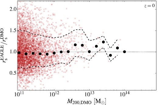
Ratio of NFW scale radii, rs, in matched relaxed haloes in the DMO and EAGLE simulations. The black points are placed at the geometric mean of the ratios in each mass bin.
Finally, the bottom panel of Fig. 11 shows the concentration of the DM only component of EAGLE haloes. We fit an NFW profile in the same way as for the total matter profiles in the panels above. As would be expected from the analysis of Fig. 8 and the fact that the outer parts of the dark haloes are well described by the NFW profile, the same trend with mass can be seen as for the DMO simulation. The best-fitting power law to the mass–concentration relation is given at the bottom of Table 3. The values of the parameters are again close to the ones obtained for both the EAGLE and the DMO simulations.
We stress that the agreement between the EAGLE and DMO simulations breaks down if we include radii smaller than 0.05Rvir in the fit. Hence, the mass–concentration relation given for EAGLE in Table 3 should only be used to infer the density profiles beyond 0.05Rvir.
4.7 Best-fitting parameter values for the new density profile
We showed in Section 4.4 that the density profiles of haloes in the EAGLE simulation are not well fit by an NFW profile in the inner regions, and we proposed equation (19) as a new fitting formula for these profiles. This new profile has two length-scales, rs and ri, where the former describes the NFW-like outer parts of the halo, and the latter the deviations from NFW in the inner regions. For lower mass haloes, these two lengths become similar, so both terms of the profile can contribute significantly to the density at all radii. We can still define the concentration of a halo in this model as R200/rs, but we would expect to obtain a different mass–concentration relation from that for the DM-only case. Fig. 13 shows this relation for relaxed EAGLE haloes. The anticorrelation seen when fitting an NFW profile is still present and we can use the same power-law formulation to describe the mass–concentration relation of our halo stacks. The values of the best-fitting parameters, given in the figure, differ significantly from those obtained using the NFW fits listed in Table 3.
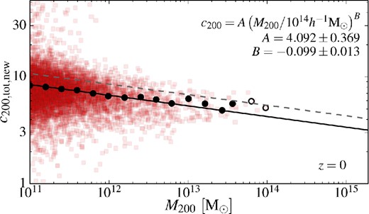
Halo concentration, c200, as a function of mass, M200, for the total matter density profiles of the EAGLE simulation using the fitting function of equation (19) and the rs parameter to define the concentration, c200 = R200/rs. The colour points are for individual haloes and the black circles for the stacked profiles in each mass bin. The solid black line is the best-fitting power law (equation 23) to the solid black circles. The best-fitting values are given in the legend at the top right. The dashed line shows the best-fitting power law to the haloes extracted from the DMO simulation fitted using an NFW profile.
We now consider the two remaining parameters of the profile described by equation (19). The inner component is characterized by two quantities, a scale radius, ri, and a density contrast, δi. We stress that this inner profile should not be interpreted as the true underlying model of the galaxy at the centre of the halo. It is an empirical model that describes the deviation from NFW due to the presence of stars and some contraction of the DM. The profiles have been fit using the procedure described in Section 4.4 using all radial bins with r > rc.
The dependence of the ri scale radius on the halo mass is shown in Fig. 14. The radius ri is roughly constant over the entire halo mass range in the simulation. The scatter is large at all masses, but there is a weak trend with mass in the low-mass regime. This regime is, however, difficult to study as may be seen in the first few panels of Fig. 8: for the smallest haloes, the effects due to baryons are small and the profile is thus closer to NFW than for the higher mass bins.
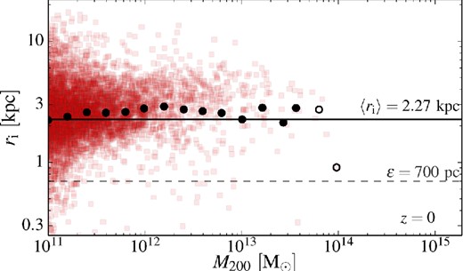
The characteristic radius, ri, of the central component as function of halo mass (equation 19) for haloes in the EAGLE simulation. The red squares correspond to all the haloes fitted individually and the overlaying black circles to the stacked haloes in each mass bin. Stacks containing less than three objects are shown as open circles. The minimum Plummer-equivalent softening length (ϵ = 0.7 kpc) is indicated by the grey dashed line at the bottom of the figure. The average value of the stacks with more than three objects is indicated by a solid black line.
The empirical profile (equation 19) tends towards an NFW profile as δi → 0 or ri → 0. We find that, for the smallest haloes, there is a degeneracy between these two parameters and the values of ri and δi can be changed by an order of magnitude (self-consistently) without yielding a significantly different σfit value. This is not a failure of the method but rather a sign that the baryonic effects on the profile shape become negligible for the lowest mass halo, at least for the range of radii resolved in this study.
The mass, Mi, is shown in Fig. 15 as a function of the halo mass, M200. The black points corresponding to the stacked profiles lie in the middle of the relation for individual haloes. The mass, Mi, increases with halo mass. For haloes with M200 ≲ 1012 M⊙, the fraction, Mi/M200, increases with M200 highlighting that the effect of the baryons is more important for the bigger haloes. This could have been expected by a careful inspection of Fig. 4, which shows that the central stellar and baryonic fractions peak at M200 ≈ 1012 M⊙. For larger haloes, the M200–Mi relation flattens reflecting the decrease in stellar fractions seen at the centre of the largest EAGLE haloes.
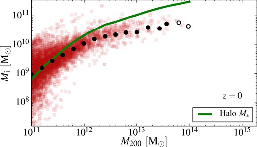
To confirm this conjecture, we plot the stellar mass–halo mass relation for the EAGLE simulation as a solid green line in the same figure (Schaye et al. 2015).1 Neglecting the two highest mass bins (open circles), the similarity between this relation and our somewhat arbitrary definition of Mi seems to indicate that the stellar mass of the haloes is related to this parameter. The definition of the mass, Mi, could also be modified to take into account other properties of the galaxy in the halo. We could, for instance, include the galaxy size (half-stellar mass radius or half-light radius, for example) instead of ri in the definition of Mi. It would then be interesting to see how this newly defined mass correlates with the galaxy's stellar mass.
4.8 A non-parametric estimate of the concentration
The definition of concentration assumes that the haloes are well fit by an NFW (or other) profile. This is the case for our sample of haloes down to radii ∼0.05Rvir, so we can safely compute the concentration of these haloes as rs > 0.05Rvir for almost all cases of interest. It is nevertheless worthwhile measuring a proxy for the concentration which does not rely on a specific parametrization of the profile. This is also more convenient for observational purposes, where a large range of radii are not always available to perform a fit. A simpler estimator of the concentration can then help constrain the models without making assumptions about the exact shape of the profile. This is particularly true for X-ray observations because it is difficult to detect X-ray emission all the way to the virial radius.
Such an estimator is given by the ratio of spherical overdensity radii R500/R2500 (e.g. Duffy et al. 2010). Both of these quantities can be obtained without assuming anything about the slope and functional form of the matter density profile. We show the value of this ratio as a function of the spherical enclosed mass, M500, in Fig. 16. The EAGLE and DMO simulations show the same trends and the differences between them are smaller than the scatter between individual haloes. As could already be seen from the profiles in Figs 6 and 8, the effect of modelling the baryons is concentrated at small radii, well within R2500.

The average ratio of the R500 and R2500 radii as a function of halo mass, M500, for both the EAGLE (red squares) and DMO (green circles) simulations.The error bars represent the 1σ scatter in the population. To ease the reading of the plot, the points with error bars have been artificially displaced by 0.02 dex towards the left and right for the EAGLE and DMO results, respectively. The black dashed line shows the expected relation for an NFW profile with the concentration–mass relation determined for the EAGLE simulation in Section 4.6.
4.9 Limitations of the subgrid model
The convergence test in subsection 4.1 demonstrated that the simulation results of interest here are converged at radii, r > rc (given by a modified version of the criterion proposed by P03) and that even at smaller radii the profiles of stacked haloes remain remarkably similar when the resolution is increased by a factor of 8 in particle mass. A halo of mass M200 ≈ 1011 M⊙ is then resolved with |$\mathcal {O}(10^5)$| particles and its stellar disc with |$\mathcal {O}(10^3)$| particles, which is enough to sample star formation histories with good accuracy and obtain a realistic galaxy population (Furlong et al. 2014; Crain et al. 2015; Schaye et al. 2015).
An interesting aspect of our simulations is that no haloes (of any mass) develop density cores in their central regions within the resolved radial range. By contrast, simulations of dwarf and even larger galaxies by a number of authors produce such cores (see references in Section 4.2 and Pontzen & Governato 2014, for a review). As shown by Navarro et al. (1996a), a physical mechanism that can produce a flattening of the inner DM density profile is the sudden removal, in a starburst, of gas that had previously contracted enough to become self-gravitating, dominate the central gravitational potential and slowly drag DM in. The subsequent loss of binding energy from the central regions by the removal of that gas on a time-scale shorter than the local dynamical time causes the DM to flow outwards resulting in a flattening of the profile to a degree that depends on the size and mass of the self-gravitating gas component. A variant of this process is apparently responsible for the formation of cores in simulations of dwarf galaxy (e.g. Governato et al. 2010) and in simulations of galaxy clusters (where the source of energy is an AGN; Martizzi et al. 2013).
An important aspect of the simulations by Governato et al. (2010) is that the assumed subgrid model adopts a higher density threshold for star formation (10-100mH · cm− 3) than we have assumed in EAGLE (a metallicity-dependent threshold with a value of 0.031mH · cm− 3 at solar metallicity that traces the density above which a cold, molecular gas phase is expected to be present; see Schaye 2004 and Schaye et al. 2015).2 Although even the high value assumed by Governato et al. (2010) is many orders of magnitude below the gas density in the star-forming cores of molecular clouds, it probably allows a substantial amount of gas to dominate the potential in the central regions prior to a starburst, as required for the Navarro et al. (1996a) mechanism to operate.3
It is not obvious a priori which, if any, of the subgrid models for star formation used to date is more appropriate, but an important virtue of the EAGLE subgrid model is that it leads to a population of galaxies with properties that agree well with a large set of observations, from the regime of dwarf galaxies to the regime of galaxy clusters (Furlong et al. 2014; Schaller et al. 2014; Crain et al. 2015; Sawala et al. 2015; Schaye et al. 2015). None of the simulations that produce cores in the DM has yet been able to demonstrate such success. Indeed, other large cosmological simulations with different subgrid models to EAGLE such as ‘Illustris’ do not appear to have produced density cores either (Vogelsberger et al. 2014). In any event, the evidence for the existence of cores in real galaxies is still a matter of lively debate, with some authors reporting cores (e.g. Salucci & Burkert 2000; Swaters et al. 2003; Simon et al. 2005; Gentile et al. 2007; de Blok et al. 2008; Kuzio de Naray, McGaugh & de Blok 2008; Oh et al. 2011), others reporting cusps (even for some of the same galaxies; e.g. Adams et al. 2014), and others arguing that current kinematical data cannot distinguish cores from cusps (at least in the case of satellites of the Milky Way for which kinematical studies on resolved stellar populations are possible; Strigari, Frenk & White 2010, 2014).
Finally, we stress that the conclusions in this paper refer only to radii larger than r > rc ≈ 1.8 kpc. Higher resolution simulations would be required to test whether our subgrid model can generate density cores on smaller scales than those resolved in this study.
5 CONCLUSIONS
The aim of this study was to characterize the mass density profiles of DM haloes in a cosmological ΛCDM simulation, which includes DM and baryons, and in which the resulting galaxy population has realistic stellar masses and sizes; we also quantified the differences with haloes in a DM-only simulation. We used the state-of-the-art EAGLE simulation from which we selected haloes above 109 M⊙ to study changes in the mass, and above 1011 M⊙ to study changes in the internal structure. Our results can be summarized as follows.
The mass, M200, of haloes is reduced by the inclusion of baryons and associated energy feedback effects. At the low-mass end, feedback from star formation expels gas and this reduces the total mass, radius, and growth factor of the halo; the reduction in mass can be as large as 30 per cent for haloes with M200 ≲ 1011 M⊙. This reduction is progressively smaller for larger haloes as the source of feedback shifts from star formation to AGN. In the EAGLE simulation, there is virtually no effect for masses M200 ≳ 1014 M⊙, but the exact value of the mass at which this happens could be larger if, as suggested by Schaye et al. (2015), more effective AGN feedback is necessary than is present in EAGLE. The reduction in mass can be described by the double-sigmoid function of equation (13), and the scatter around the mean by the formula of equation (14).
The circular velocity curves of the EAGLE haloes are in excellent agreement with observational data for galaxies with stellar mass ranging from 109 to 5 × 10¹¹ M⊙ (corresponding to halo masses in the range 1011 ≲ M200/M⊙ ≲ 1013).
The radial density profiles of EAGLE haloes over the radial range [0.05Rvir, Rvir] are very similar to the profiles of haloes in DM-only simulations and are well described by the NFW formula. Halo concentrations estimated by fitting NFW profiles over this range are also very similar to the DM-only case.
The central regions of haloes more massive than M200 ≳ 1012 M⊙, on the other hand, are dominated by the stellar component. The presence of these baryons causes a contraction of the halo, enhancing the density of DM in this region. The variation in profile shape is greatest for haloes in the mass range M200 = 1012–1013 M⊙ where the stellar mass fraction peaks (as does the total baryonic mass fraction within 0.05Rvir).
The radial density profiles of the EAGLE haloes can therefore be well fit (over the radial range resolved in the simulation) by the sum of an NFW profile, which describes the outer, DM-dominated regions, and an NFW-like profile with a sharper bend, which describes the combined effect of the presence of stars and the contraction of the DM halo (equation 19). Of the two additional parameters required in this fit, one, ri, is approximately constant with halo mass, while the other one, the characteristic inner mass scale, Mi, scales with halo mass in a similar way to the stellar mass of the central galaxy.
The way in which galaxy formation affects the host haloes is a problem that can only be reliably addressed with simulations of the kind we have described here. However, it is clear that the nature of these effects is sensitive to the way in which the baryon physics are implemented, particularly to the subgrid models for feedback from star formation and AGN. The EAGLE simulations have the great advantage that the subgrid models have been calibrated so that the simulation reproduces the local galactic stellar mass function as well as the distribution of galaxy sizes, and they also reproduce a wide variety of other observations. This lends a certain degree of credibility to our results and it would be interesting to compare them with other simulations that assume different subgrid models but achieve similarly good matches to observables over a large range of halo masses. A limited comparison of this kind is carried out in Appendix A1.
The simulations investigated here do not have enough resolution to study dwarf galaxies for which there is much discussion regarding the formation of central cores in the DM density distribution (for a review, see Pontzen & Governato 2014). However, the related high-resolution simulations of the Local Group by Sawala et al. (2015), which use essentially the same subgrid models as EAGLE, do resolve dwarfs. The behaviour of these smaller haloes simply continues to smaller masses the trends seen here: the haloes become increasingly DM-dominated and remain well described by the NFW profile.
We are grateful to Lydia Heck and Peter Draper without whose technical expertise and support this work would have not been possible. RAC is a Royal Society University Research Fellow. This work was supported in part by an STFC Consolidated grant to Durham University and by the European Research Council through ERC Grants Cosmiway (GA 267291), GasAroundGalaxies (GA 278594) and Cosmocomp (GA 238356) and also the Inter-university Attraction Poles Programme initiated by the Belgian Science Policy Office ([AP P7/08 CHARM]). This work was also sponsored by the Dutch National Computing Facilities Foundation (NCF), with financial support from the Netherlands Organization for Scientific Research (NWO). The EAGLE simulations used the DiRAC Data Centric system at Durham University, operated by the Institute for Computational Cosmology on behalf of the STFC DiRAC HPC Facility (www.dirac.ac.uk). This equipment was funded by BIS National E-infrastructure capital grant ST/K00042X/1, STFC capital grant ST/H008519/1, and STFC DiRAC Operations grant ST/K003267/1 and Durham University. DiRAC is part of the National E-Infrastructure. We acknowledge PRACE for resources on the Curie supercomputer in France.
Note that the EAGLE simulation reproduces abundance matching results (Schaye et al. 2015).
A significant number of stars in EAGLE, however, form from gas at much higher densities that the threshold; see Crain et al. (2015).
It is unclear whether cold, dense star-forming clouds in a multiphase ISM (McKee & Ostriker 1977) would contain enough mass to dominate the central potential of the halo.
REFERENCES
APPENDIX A: UNCERTAINTIES DUE TO THE SUBGRID MODELS
As discussed by Schaye et al. (2015), cosmological hydrodynamical simulations require subgrid models whose parameters have to be calibrated against a set of observables. In the case of the EAGLE suite of simulations, the observations used are the z = 0 galaxy stellar mass function, the galaxy mass–size relation and the stellar mass–BH mass relation. Using only a subset of these observables, it is possible to find different values of the subgrid model parameters that match the galaxy stellar mass function (Crain et al. 2015). Hence, it is important to assess whether the results presented here depend on these parameters or on the resolution of the simulation.
A1 Changes in the AGN model parameters
One of the models that matched the selected set of observables is the EAGLE model AGNdT9-L050N0752, which is very similar to the EAGLE-Ref model used in the rest of this paper but whose parameters have been calibrated to match the group gas fractions and X-ray luminosities better (Schaye et al. 2015). In this model, the galaxy masses and sizes are very similar to the Ref model and we have verified that the DM halo profiles extracted from that model are very close to the ones shown in Section 4.2 for the halo mass range represented in this simulation (M ≲ 2 × 10¹³ M⊙).
In Section 3.1, we discussed the difference in halo masses between the AGNdT9 simulation and its DMO equivalent and showed that the ratio reached unity only for more massive haloes than in EAGLE-Ref model. This is, in part, caused by the lower baryon fractions that these haloes have. Fig. A1 shows the baryon (top panel) and stellar (bottom panel) fractions for haloes extracted from the EAGLE-Ref simulation (black circles) and from the EAGLE-AGNdT9 model (red squares). The stellar fractions are comparable in both models, with any differences laying well within the large halo-to-halo scatter. The baryon fractions in group-like haloes (1013 M⊙ < M200 < 1014 M⊙), however, are systematically lower, by as much as 20 per cent, in the EAGLE-AGNdT9 model. This difference is reflected in the observed shift in the best-fitting parameter, M23, in equation (13) between the two models. The difference vanishes for the central regions of the haloes. The baryon and stellar fractions within 0.05R200 are similar in both simulations indicating that the difference in the AGN treatment has mostly lead to a change in the structure of the gas outside galaxies, impacting on the inferred X-ray luminosities (Schaye et al. 2015).
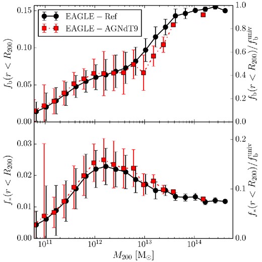
Baryon fraction, fb = Mb/M200 (top panel), and stellar fraction, f* = M*/M200 (bottom panel), within R200, as a function of halo mass for the EAGLE-Ref model (black circles) and the EAGLE-AGNdT9 model (red squares). The error bars show the rms halo-to-halo scatter in each mass bin. The baryon fractions in the haloes more massive than 1013 M⊙ are lower in the AGNdT9 model.
