


Abstract
A series of optical and one near-infrared nebular spectra covering the first year of the Type Ia supernova SN 2011fe are presented and modelled. The density profile that proved best for the early optical/ultraviolet spectra, ‘ρ-11fe’, was extended to lower velocities to include the regions that emit at nebular epochs. Model ρ-11fe is intermediate between the fast deflagration model W7 and a low-energy delayed-detonation. Good fits to the nebular spectra are obtained if the innermost ejecta are dominated by neutron-rich, stable Fe-group species, which contribute to cooling but not to heating. The correct thermal balance can thus be reached for the strongest [Fe ii] and [Fe iii] lines to be reproduced with the observed ratio. The 56Ni mass thus obtained is ∼0.47 ± 0.05 M⊙. The bulk of 56Ni has an outermost velocity of ∼8500 km s−1. The mass of stable iron is ∼0.23 ± 0.03 M⊙. Stable Ni has low abundance, ∼10−2 M⊙. This is sufficient to reproduce an observed emission line near 7400 Å. A sub-Chandrasekhar explosion model with mass 1.02 M⊙ and no central stable Fe does not reproduce the observed line ratios. A mock model where neutron-rich Fe-group species are located above 56Ni following recent suggestions is also shown to yield spectra that are less compatible with the observations. The densities and abundances in the inner layers obtained from the nebular analysis, combined with those of the outer layers previously obtained, are used to compute a synthetic bolometric light curve, which compares favourably with the light curve of SN 2011fe.
INTRODUCTION
Given the importance of Type Ia supernovae (SNe Ia), one fundamental question concerns their origin. There is strong evidence that they are the explosion of compact stars, most likely carbon-oxygen (CO) white dwarfs (WDs). Such stars can undergo thermonuclear explosive burning which results in the production of radioactive 56Ni, whose decay powers the SN luminous output, and other elements along the α-chain. Apart from 56Ni, the element which is produced most abundantly is silicon, whose presence characterises the spectra of SNe Ia at early times (Benetti et al. 2005; Nugent et al. 2011; Folatelli et al. 2012; Parrent et al. 2012). We know that 56Ni is produced in variable amounts (Mazzali et al. 2007a), and that the relation between 56Ni, luminosity, and opacity (Pinto & Eastman 2000; Mazzali et al. 2001) shapes the light curves of SNe Ia, which are to first order a one-parameter family where broader light curves belong to more luminous SNe (Phillips 1993). The explosion is thought to start when the WD reaches a central temperature of ∼109 K, which happens when its mass approaches the Chandrasekhar limit, or it may be triggered by accretion or merger events in lower-mass WDs.
What we do not know for sure, despite much effort, is how the CO–WD reaches such a large mass, and how it then explodes. We need to establish this so that we can then tackle the problem of how the explosion can produce SNe with different 56Ni content and hence different luminosity. Popular models for pushing the WD mass close to the Chandrasekhar limit involve transfer of mass from a non-degenerate binary companion (main sequence or red giant), the single-degenerate (SD) scenario, or the merger of two WDs, the double-degenerate (DD) scenario. Both scenarios have pros and cons.
The SD scenario ensures repeatability, a constant exploding mass, and a spread of ages, but it is supposed to involve hydrogen accretion, which should lead to the detection of H, either in the outer layers as a leftover of the accreting material or at low velocities as is expected of H stripped from the companion by the SN ejecta (Marietta, Burrows & Fryxell 2000; Pakmor et al. 2011). However, only rarely has H been directly detected in SNe Ia (Silverman et al. 2013). Interestingly, in these cases much H is seen, such as in SN 2002ic (Hamuy et al. 2003; Deng et al. 2004) or PTF11kx (Dilday et al. 2012). Also, the identification of a surviving companion is not certain (Ruiz-Lapuente et al. 2004; Kerzendorf et al. 2009).
The DD scenario may occur more frequently. It is, however, unclear how many merger events actually exceed a combined mass of about the Chandrasekhar mass. The proposed scenarios, violent mergers (Pakmor et al. 2011) or collisions (Rosswog et al. 2009; Thompson 2011; Kushnir et al. 2013), produce diverse outcomes depending on the initial conditions. The question then is whether they look like a typical SNe Ia, especially in view of the fact that they involve large asymmetries because ignition happens at the point of contact rather than at the highest density.
In a further twist, the possibility that WDs below the Chandrasekhar limit also explode if they accrete He-rich matter from a companion has also been proposed (Livne & Arnett 1995). This, the sub-Chandra scenario, may again lead to a different set of observed properties (e.g. Nugent et al. 1997; Woosley & Kasen 2011).
Since all of these scenarios are based on solid physical ideas, it is perfectly possible that they are all actually verified in nature. Is this indeed the case? Does this add to the uncertainty in our use of SNe Ia as distance indicators? While the latter is a question that can also be addressed by using large samples of SNe, the former is one that requires the accurate study of a few, well-observed SNe.
The biggest differences among explosion models are expected to be found either at high velocities (presence of circumstellar matter, amount of material at high velocity as an indication of kinetic energy, metal content of the progenitor, unburned material from the progenitor or the companion), or at the lowest ones (central densities, composition, material dragged from companion upon impact). Different epochs in a SN's evolution yield different information. Early-time data can be used to infer the size of the progenitor, possibly that of the companion (in the SD scenario), and the properties of the outer layers of the exploding star, which may not be affected by thermonuclear burning and may thus carry information about the accreting material. Observations over the first month or so tell us about general properties: the light-curve shape (mass, opacity), ejecta velocity (kinetic energy), and composition of the outer layers [extent of 56Ni, intermediate-mass elements (IMEs)]. Correlations have been found among these quantities, appearing to suggest some regularity.
However, if information about the central regions is required, one has to wait for the nebular phase. At late times (∼1 yr), opacities are low and it is possible to explore the lowest-velocity material. This corresponds to the highest densities, and hence it should bear the trace of the ignition and the outcome of the explosion.
SN 2011fe (Nugent et al. 2011) is the perfect candidate for accurate studies. When it was discovered it was the nearest SN Ia in almost 40 yr. It has been observed extensively at frequencies from the radio (Chomiuk et al. 2012; Horesh et al. 2012), to the far-infrared (IR) with Herschel (Johansson, Amanullah & Goobar 2013), to the mid-IR with Spitzer (McClelland et al. 2013), to the near-IR (Matheson et al. 2012), to the optical (Li et al. 2011; Nugent et al. 2011; Richmond & Smith 2012; Munari et al. 2013; Pereira et al. 2013; Shappee et al. 2013; Tsvetkov et al. 2013), to the ultraviolet (UV) with Swift (Nugent et al. 2011; Brown et al. 2012) and with the HST (Foley & Kirshner 2013; Mazzali et al. 2014), to the X-rays with Swift (Horesh et al. 2012; Margutti et al. 2012) and Chandra (Margutti et al. 2012), and finally to the gamma rays (Isern et al. 2013).
SN 2011fe was a normal SN Ia hosted in a spiral galaxy, M101. The early discovery of the SN by the PTF collaboration allowed a good estimate to be made of the time of explosion (Nugent et al. 2011, revised by Piro & Nakar 2013 and Mazzali et al. 2014), and also made it possible to estimate the size of the exploding star to be Rprog ≲ 0.02 R⊙ (Bloom et al. 2012). The early-time light curve did not reveal the signature expected from a shocked companion, contrary to predictions if this were a sizeable star (Kasen 2010; Nugent et al. 2011). Early-time spectra exhibit traces of carbon in the outer layers (Parrent et al. 2012; Mazzali et al. 2014) and are consistent with the low metallicity of the host galaxy (Mazzali et al. 2014). The spectra have been claimed to be consistent with both an SD and a DD scenario (Röpke et al. 2012). In the outer layers, a density intermediate between the fast deflagration model W7 and a low-energy delayed detonation was found to be the best solution for the optical/UV spectra (Mazzali et al. 2014). Merger models and sub-Chandrasekhar-mass models seem to have lower densities in the inner layers, and a nebular study can help determining how well they might reproduce the properties of SNe Ia.
In the following, the nebular-phase data for SN 2011fe are presented (Section 2). We show models of the optical spectra in Section 3 using the density profile derived from the early-time spectra. In Section 4, we extend the models to the near-infrared (NIR) and discuss alternative models. A discussion (Section 5) and conclusion (Section 6) follow.
NEBULAR SPECTRA OF SN 2011FE
A series of 10 nebular spectra of SN 2011fe was taken over the period 2012 March to August. An observing log can be found in Table 1.
Observing log for the nebular spectra of SN 2011fe.
| Ut Date | Telescope | Instrument | Wavelength |
|---|---|---|---|
| coverage | |||
| 2012 Mar 2 | WHT | ISIS | 3500–10 000 Å |
| 2012 Mar 24 | LBT | MODS | 3300–10 000 Å |
| 2012 Apr 2 | Lick | Kast | 3450–10 300 Å |
| 2012 Apr 23 | Lick | Kast | 3450–10 200 Å |
| 2012 Apr 27 | LBT | MODS | 3300–10 000 Å |
| 2012 May 1 | LBT | Lucifer | 1.17–1.31 μm |
| 2012 May 1 | LBT | Lucifer | 1.55–1.74 μm |
| 2012 May 1 | LBT | Lucifer | 2.05–2.37 μm |
| 2012 May 26 | WHT | ISIS | 3500–9500 Å |
| 2012 Jun 12 | LBT | MODS | 3300–10 000 Å |
| 2012 Jun 25 | WHT | ISIS | 3500–10 600 Å |
| 2012 Jul 17 | Lick | Kast | 3450–10 300 Å |
| 2012 Aug 21 | WHT | ISIS | 3500–10 000 Å |
| 2012 Aug 23 | Lick | Kast | 3450–10 200 Å |
Nebular models.
| Date | Epoch | M(CO) | M(IME) | M(56Ni) | M(54Fe) | M(58Ni) | M(NSE) | v(1-zone) |
|---|---|---|---|---|---|---|---|---|
| (rf d) | (M⊙) | (M⊙) | (M⊙) | (M⊙) | (M⊙) | (M⊙) | (km s−1) | |
| 2012 Mar 2 | 192 | 0.24 | 0.42 | 0.41 | 0.29 | 0.007 | 0.71 | 8000 |
| 2012 Apr 2 | 223 | 0.24 | 0.42 | 0.44 | 0.26 | 0.007 | 0.71 | 7900 |
| 2012 Apr 23 | 244 | 0.24 | 0.42 | 0.45 | 0.25 | 0.006 | 0.70 | 7900 |
| 2012 Apr 27 | 248 | 0.24 | 0.42 | 0.46 | 0.24 | 0.004 | 0.70 | 7800 |
| 2012 May 1 | 252 | 0.24 | 0.41 | 0.48 | 0.22 | 0.004 | 0.69 | 7800 |
| 2012 May 26 | 277 | 0.24 | 0.41 | 0.46 | 0.22 | 0.007 | 0.70 | 7900 |
| 2012 Jun 25 | 307 | 0.24 | 0.41 | 0.48 | 0.21 | 0.007 | 0.70 | 7600 |
| 2012 Jul 17 | 329 | 0.24 | 0.39 | 0.51 | 0.22 | 0.007 | 0.73 | 7500 |
| 2012 Aug 22 | 364 | 0.24 | 0.38 | 0.54 | 0.18 | 0.008 | 0.72 | 7700 |
Four spectra were taken with the William Herschel Telescope (WHT) using the Intermediate dispersion Spectrograph and Imaging System (ISIS). ISIS is a dual-arm spectrograph; we used the R158R grating and GG495 order blocker (red arm), as well as the R300B grating (blue arm) and the 5300 Å dichroic, giving a wavelength coverage of ∼3500–10 000 Å. Four spectra were taken using the Lick Observatory 3-m Shane telescope and the Kast dual-channel spectrograph (Miller & Stone 1993). The 600/4310 grism was used in the blue arm and the 300/7500 grating in the red arm, giving a wavelength coverage of 3450–10 200 Å.
All of the Lick spectra were reduced using standard techniques (e.g. Silverman et al. 2012). Routine CCD processing and spectrum extraction were completed with iraf.1 We obtained the wavelength scale from low-order polynomial fits to calibration-lamp spectra. Small wavelength shifts were then applied to the data after cross-correlating a template sky to the night-sky lines that were extracted along with the SN. Using our own idl routines, we fit spectrophotometric standard-star spectra to the data in order to flux calibrate our spectra and to remove telluric lines (Wade & Horne 1988; Matheson et al. 2000).
Spectra of SN 2011fe were obtained with the Large Binocular Telescope (LBT) and Multi-Object Dual Spectrograph (MODS; Pogge et al. 2012) on three nights in 2012: March 24, April 27, and June 12 (ut dates are used throughout this paper). Details of the data acquisition and reduction can be found in Shappee et al. (2013).
NIR spectra were also obtained with the LBT LUCIFER spectrograph (Seifert et al. 2003) on 2012 May 1, close to the date of one of the MODS optical spectra. We used the 210 line mm−1 grating and 1.0 arcsec-wide slit, resulting in a resolution of 4000 in the J band. Data were taken at three grating tilts to obtain spectra in the J, H, and K bands. Consecutive exposures were dithered along the slit and used to subtract the sky background. Images at each slit position were then combined and extracted using the iraf ‘twodspec’ package, and the two spectra were averaged to create the final spectrum. The spectra were wavelength calibrated using night-sky emission lines, and telluric absorption features were removed using a spectrum of the A0 V star HIP67848 taken immediately after the SN spectra. The NIR magnitudes of HIP67848 were then used to flux calibrate the spectra of SN 2011fe.
An acquisition image of SN 2011fe was obtained in the J band with LUCIFER. Using Two-Micron All-Sky Survey (2MASS) catalogue in the field we estimate the brightness of the SN to be J = 17.20 ± 0.06 mag.
The spectra were reduced using custom-written pipelines based on standard procedures in iraf and idl, broadly following the reduction procedures outlined by Ellis et al. (2008), including flux calibration and telluric-feature removal. All spectra were observed at the parallactic angle (Filippenko 1982) in photometric conditions. ‘Error’ spectra are derived from a knowledge of the CCD properties and Poisson statistics, and are tracked throughout the reduction procedure. The spectra are also rebinned (in a weighted way) to a common dispersion, and the two arms of the spectrographs joined.
The nebular spectra of SN 2011fe have been checked against the late-time broad-band photometry of Tsvetkov et al. (2013). The broad-band magnitudes at the epochs of the nebular spectra were derived, for each band, from a linear fit of the available photometric points on the exponentially declining tail of the light curve. The flux calibration of the spectra was then checked against the photometry using the iraf task stsdas.hst_calib.synphot.calphot. Next, we locked the absolute flux scale of each spectrum, normalizing the synthesized BVRI magnitudes from the spectrum to the interpolated broad-band magnitudes. The 2012 August 21 and 23 spectra were combined into a single spectrum to improve the signal-to-noise ratio.
MODELLING
We modelled the nebular spectra of SN 2011fe using our well-tested SN nebular code. The code is based on approximations developed by Axelrod (1980), and it has been developed and discussed in various papers (Mazzali et al. 2001; Mazzali et al. 2007b). The SN ejecta are divided into a number of spherical shells, whose density reflects that of an explosion model and whose composition can be varied arbitrarily. The ejecta size and density are rescaled to the epoch of the desired model assuming homologous expansion. 56Ni decay provides the heating. In the first step of the procedure, γ-rays and positrons are emitted according to the distribution of 56Ni. Their propagation is followed with a Monte Carlo scheme (Cappellaro et al. 1997). While γ-rays can travel a long way before being absorbed in the late-time low-density SN ejecta, positrons mostly deposit their energy locally. Deposition of the energy carried by γ-rays and positrons determines the heating rate. Under nebular conditions, this collisional heating is balanced by cooling via line emission. The ionization and excitation of relevant species is computed assuming non-local thermodynamic equilibrium, balancing heating and cooling in an iterative scheme. When convergence is reached, line emissivity is transformed into an emission-line spectrum. An emitted spectrum is computed for every shell, and the final emerging spectrum is the sum of the contributions from all shells.
A successful model should be able to reproduce the evolution of the spectrum with time, reflecting the decreasing heating rate and deposition. Mazzali et al. (2014) showed that the early-time spectra of SN 2011fe cannot be satisfactorily reproduced with available SN Ia explosion models, and proposed a density distribution characterized by a small but non-zero mass at high velocities, above ∼23 000 km s−1 (see Fig. 1). This model was shown to be able to reproduce both the optical and UV spectra simultaneously. The early-time study could not explore the deepest parts of the ejecta, which are optically thick at early epochs. Here, we extend the results of Mazzali et al. (2014) and explore the deepest regions of the ejecta.
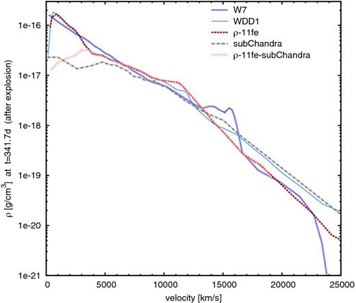
Density structures used in this paper: W7 (blue), delayed-detonation model WDD1 (light blue, solid), sub-Chandra model CDT3 (grey), ρ-11fe (red), and a sub-Chandra ρ-11fe model with M = 1.2 M⊙ (light red).
Mazzali et al. (2014) concluded that in SN 2011fe some ∼0.4 M⊙ of 56Ni are located at v ≳ 4500 km s−1. Estimates of the total 56Ni mass for SN 2011fe suggest a value close to 0.5 M⊙ (Pereira et al. 2013). If correct, this implies that only a small fraction of all 56Ni is located at low velocities. If the total ejected mass of SN 2011fe was close or equal to the Chandrasekhar mass, using the density structure ρ-11fe leaves ∼0.25 M⊙ below 4500 km s−1. Additionally, because of limitations of our early-time code caused by the lower boundary blackbody assumption (e.g. Mazzali et al. 1993), abundances in layers where 56Ni is dominant may not be fully reliable. In SN 2011fe this affects the region below ∼7000 km s−1. In any case, we adopted the abundances determined by Mazzali et al. (2014) as our initial distribution, and adapted those in the region below 4500 km s−1 in order to fit the spectra. The density structure of model ρ-11fe, as well as those of other models used in this paper, are shown in Fig. 1.
Assuming that the spectra are properly calibrated in flux (there may be some uncertainty when spectra were taken at different telescopes, see below), the overall flux level should reflect the total mass of 56Ni. An important remark here is that even in the case of SN 2011fe the uncertainty in flux calibration can account for an uncertainty in the luminosity level of up to ∼10 per cent. In the modelling, we adopted for SN 2011fe a distance of 6.4 Mpc (distance modulus μ = 29.04 mag; Shappee & Stanek 2011, find μ = 29.04 ± 0.05 (random) ±0.18 (systematic) mag), and reddenings E(B − V) = 0.014 mag in the host galaxy and E(B − V) = 0.009 mag in the Milky Way (Schlegel, Finkbeiner & Davis 1998; Patat et al. 2013).
The main results of our models are listed in Table 2. We find that the nebular spectra of SN 2011fe require on average a 56Ni mass of ∼0.47 M⊙. This is consistent with previous estimates based on the peak of the light curve (Pereira et al. 2013). Our set of nebular models is shown in Figs 2 and 3, and Table 1 summarizes the main results. There seems to be a tendency for the 56Ni mass to increase for later-time spectra. This may be caused by inaccuracies in our description of positron escape, since little is known about positron deposition (Cappellaro et al. 1997), but in test models with full positron trapping we are getting similar results. Another possibility is that too much IR flux is produced by our models for the later epochs. There may be indications of this in the Fe-dominated emission features in the red, which are increasingly overestimated by the model spectra, while the emission at 9400–9800 Å is not reproduced in our models. These are high-lying Fe ii transitions. One possibility is that the collision strengths of these and other weak lines are not well determined. Overall, however, given the poor fitting of some features, possible uncertainties in flux calibration, and the neglect of radiative-transfer effects, we regard our 56Ni mass estimate to be within the uncertainties.
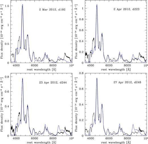
Synthetic spectra based on the ρ-11fe model (blue) compared with observed spectra (black): earlier spectra.
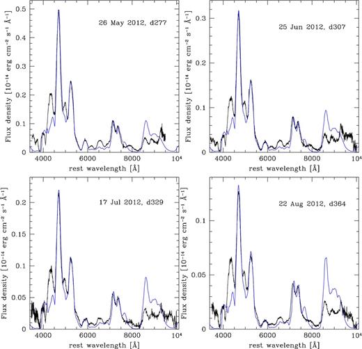
Synthetic spectra based on the ρ-11fe model (blue) compared with observed spectra (black): later spectra.
Another region that is poorly reproduced is the emission near 4250 Å. Several moderately strong [Fe ii] lines are present there, including lines at 4244 Å, 4277 Å, and 4416 Å, but their combined strength is only about half of what is observed. This may be due to problems with collision strengths, A-values, or it may indicate the presence of some other species which is not considered in our models. The same is true for the narrow emission near 5000 Å.
The element distribution determined from the early-time spectra is compatible with the late-time models. These are really only sensitive out to v ≈ 8000 km s−1, which is the width of the emission lines. Fitting the Fe emission lines, we find a roughly constant width, perhaps with a slight tendency to decrease with time. The characteristic width at epochs of ∼1 yr is ∼7600 km s−1. Based on a relation between emission-line width and light-curve shape (Mazzali et al. 1998), we expect for SN 2011fe a full width at half-maximum intensity of the strongest Fe line blend of ∼12 500 km s−1, and this is indeed what we measure.2 This corresponds to a normal SN Ia, but appears to be somewhat narrow for the 56Ni mass and the light-curve shape (Δm15(B) = 1.07 ± 0.06 mag; McClelland et al. 2013).
Our total 56Ni mass is only slightly larger than the mass determined from our early-time analysis at velocities v > 4500 km s−1. Only an additional ∼0.1 M⊙ of 56Ni is found to be located at v < 4500 km s−1. As we mentioned, model ρ-11fe has ∼0.25 M⊙ of material below 4500 km s−1. This means that ∼0.15 M⊙ of material at low velocity is not 56Ni, but rather stable nuclear statistical equilibrium (NSE) species. Two major species are predicted to be synthesized in n-rich burning: 54Fe and 58Ni, both of which are stable isotopes. We have a direct handle on the abundance of stable Ni from the emission line near 7400 Å, which is normally identified as [Ni ii] λλ7380, 7410. Indeed, the small emission seen in SN 2011fe near 7400 Å can only be reproduced if some Ni is present at the lowest velocities. Given the advanced epoch, this must be stable Ni, presumably 58Ni. This is produced from 54Fe in the so-called alpha-rich freezeout phase via 54Fe (α, γ) 58Ni during the early expansion. However, the broad emission in that region is dominated by other lines, [Fe ii] λλ7388, 7452 and [Ca ii] λλ7291, 7324. Only a very small mass of 58Ni is required to reproduce the small emission that corresponds in wavelength to the [Ni ii] lines. On average, a value of ∼0.008 M⊙ of 58Ni, confined below v ≈ 4000 km s−1 and concentrated at the lowest velocities, is sufficient. Even at the lowest velocities, the abundance of 58Ni never exceeds 10 per cent. This means that most of the mass at low velocities is composed of Fe. Again, this Fe cannot all come from 56Ni decay, because if it did the SN luminosity would be too high. We presume that this is mostly 54Fe.
Although we cannot distinguish 54Fe from directly synthesized 56Fe, the latter is supposed to be produced at low Y, inside the 56Ni region (Iwamoto et al. 1999), which is not where we find it to be located in our modelling. This is a common feature in SNe Ia (Stehle et al. 2005; Mazzali et al. 2008; Tanaka et al. 2011; Sasdelli et al. 2014), and it may indicate a higher Ye than predicted by models such as W7. The presence of stable Fe helps keeping the ionization degree sufficiently low that the correct relative contribution of [Fe ii] and [Fe iii] lines is achieved in our models. We showed in other work that if this central density is low, ionization becomes too high and [Fe iii] lines dominate, leading to a strong 4800 Å emission (Mazzali et al. 2011). If the density is even lower, only [Fe iii] lines are produced and the emission-line spectrum changes nature. This seems to be a feature of the fastest declining SNe Ia (Mazzali & Hachinger 2012). The total mass of stable Fe (obtained by adding material already diagnosed at high velocities by Mazzali et al. 2014, which is necessary to reproduce Fe lines at early times, when 56Ni has not yet decayed to 56Fe, and stable Fe at low velocities as determined here) is on average ∼0.23 M⊙. This is in line with the results of Mazzali et al. (2007a) and Kasen & Woosley (2007).
A plot of our abundance distribution is shown in Fig. 4. This compares favourably with one-dimensional (1D) Chandrasekhar-mass models based on the SD scenario, where ignition occurs near the centre of the WD at high density, and a sufficiently high temperature is achieved that n-rich isotopes can be synthesized.
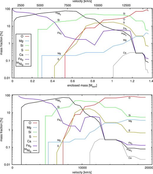
Abundance distribution in the ejecta of SN 2011fe. The elements that are shown are those that can be inferred from spectroscopic modelling of Mazzali et al. (2014). The top panel is linear with respect to mass, the bottom panel with respect to velocity.
The near-infrared
We mentioned that as time goes on, the flux is expected to shift to the infrared. We do have one epoch of NIR spectroscopy, obtained with the LBT on 2012 May 1. This spectrum can be combined with the optical spectrum obtained on 2012 April 27. In Fig. 5, we show our model for that epoch, now extending to the NIR. The model reproduces the J- and K-band spectrum reasonably well, while the flux in the H band is too low. This is in part because [Si i] 1.6 μm is overestimated, the result of 56Ni being in close contact with Si, but we also seem to somewhat overpredict the Fe emission in that region.
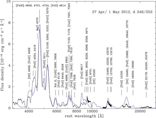
Synthetic spectrum based on the ρ-11fe model (blue), now also showing the IR. The observed IR spectrum (1 May 2012) is given along with the optical part (27 Apr 2011). The strongest lines in the model, as well as lines that match observed features in wavelength but possibly not strength, are labelled.
It is possible that a sharper velocity separation between 56Ni and IMEs may be required than the results of Mazzali et al. (2014) suggest. We tested this in a model, but the resulting spectrum still showed too much flux at 1.6 μm. Using a three-dimensional (3D) approach may be useful, concentrating 56Ni in blobs or clumps from which γ-rays escape less successfully. On the other hand, while this may help, γ-rays escape quite easily at the low densities that in general characterize the nebular regime, so the overdensity would probably have to be quite large.
The other possibility is that the density in the inner region may still be somewhat too high. In the case of SN 2003hv, a sharp reduction of the NIR flux was obtained when the central densities were decreased, shifting the flux from [Fe ii] to [Fe iii] lines. The ratio of these two ions in the optical is correctly reproduced for SN 2011fe, however, so we do not expect that the density can be reduced by a large amount. In any case, we can test this possibility using sub-Chandrasekhar-mass models.
sub-Chandrasekhar-mass models
In order to verify the need for a core of stable NSE elements, we tested a sub-Chandrasekhar-mass model. In such models, explosive burning begins at the outside, typically following the accretion of He-rich material from a companion. Most models suggest that a secondary detonation can be triggered within the WD, which can be incinerated even if its mass is significantly below the Chandrasekhar limit (Livne & Arnett 1995; Fink et al. 2010). However, because the density never reaches the high values typical of near-Chandrasekhar-mass WDs, n-rich nucleosynthesis is not expected to take place. Models are characterized by low central densities.
We used the density and abundance distribution of a 1D sub-Chandrasekhar-mass model from the set presented by Shigeyama et al. (1992). We selected model CDT3, which yields a 56Ni mass of 0.50 M⊙, in agreement with the estimated value. The total mass of the model is ∼1 M⊙. The mass of stable Fe-group isotopes, 54Fe and 58Ni, is very small, ∼0.003 M⊙ each. IMEs are present with significant abundances: Si, ∼0.21 M⊙ and S, ∼0.12 M⊙. Some unburned oxygen is also present, ∼0.07 M⊙. The density structure of this model is shown in Fig. 1.
The corresponding synthetic spectrum computed for day 248 is shown in Fig. 6. It is characterized by high ionization, as shown by the ratio of [Fe iii] and [Fe ii] lines: the [Fe iii]-dominated emission near 4800 Å is much stronger than the [Fe ii]-dominated emission near 5200 Å. This is reminiscent of SN 2003hv, and is the result of the low central density (Leloudas et al. 2009; Mazzali et al. 2011). Elsewhere, the small Si mass, its separation from 56Ni, and the lack of Fe ii means that the synthetic line at ∼ 1.6 μm is now weaker than the observed one. However, other synthetic [Fe ii] lines, such as those near 8800 Å, are still too strong, suggesting a problem with collision strengths or, less likely, A-values. On the other hand, the [Ni ii] line is no longer reproduced. Also, very noticeably, the Ca abundance is much too high, as shown by the strength of the emission near 7200 Å. This demonstrates that a model which is significantly sub-Chandrasekhar is not appropriate for SN 2011fe. It is much more difficult to establish whether a model which is just below the Chandrasekhar mass can also be ruled out. This mostly depends on the exact nucleosynthesis. It also confirms that stable Fe is required in order to reproduce the spectra.
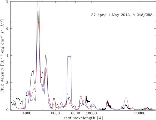
Sub-Chandra models: CDT3 (blue) and a model with M = 1.26 M⊙ (red). The observed spectrum is shown in black.
As an alternative, we constructed a sub-Chandrasekhar model with a larger mass. In this test model the total mass is 1.26 M⊙, the stable Fe content is small but not zero (0.12 M⊙), and the 58Ni mass is 0.43 M⊙, consistent with our results above. The synthetic spectrum (Fig. 6) shows again the problem of high ionization, although to a lesser extent. The best results is obtained when the mass approaches MCh and the stable Fe content is close to 0.2 M⊙.
Where is the stable Fe?
Having established that a high central density is needed, and that the presence of a significant amount of 54Fe and stable 56Fe produced at burning (Iwamoto et al. 1999) appears to be necessary, we can address the question of its location. Recent 3D delayed-detonation models suggest that n-rich NSE species produced in the deflagration phase rise because of their buoyancy and end up expanding at higher velocities than 56Ni when the simulation is performed in 3D. This leads to an inverse structure, where 56Ni is located inside n-rich NSE species (Seitenzahl et al. 2013).3 In order to assess the effect of this, we simulated spectrum formation using the ρ-11fe density structure but moving stable Fe and Ni above 56Ni in velocity. This process requires a moderate rescaling of the 56Ni mass to obtain the same luminosity, because when 56Ni is located deeper in the ejecta γ-rays deposit more efficiently. The flux level of the nebular spectrum can be reproduced for a 56Ni mass of only 0.34 M⊙. The mass of stable Fe becomes 0.43 M⊙, and 58Ni slightly increases to 0.01 M⊙. The resulting model is shown in Fig. 7.
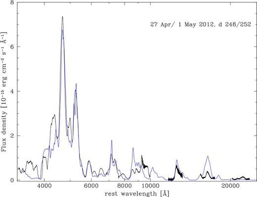
Synthetic spectrum for the Ni-Fe inversion model (blue). The observed spectrum is shown in black.
Although the model has reasonable features, three areas cause concern. First, all Fe lines are narrow. This is because there is too little 56Ni at high velocity, and the Fe that is located there is not efficiently heated by the γ-rays, which are emitted very deep in the ejecta. Increasing the mass of 56Ni would help, but the flux would be too high. Additional mixing may fix this problem, but it may take us back towards a situation where 54Fe is below 56Ni. Secondly, the ratio of Fe lines now favours Fe ii. This is not surprising, since radiation comes predominantly from the densest, innermost regions, where recombination is most effective. The ratio of the two strongest emission lines, whose atomic data are probably best known, is a driving parameter to establish the success of a model. Finally, the 56Ni mass is in rather strong disagreement with the value derived from the peak of the light curve. Combining the smaller 56Ni mass with the fact that the diffusion time of the optical photons can only increase if they are produced deeper in the ejecta, as would be the case if 56Ni were located at the lowest velocities, this ad hoc model is not expected to reproduce the observed light curve.
In conclusion, the nebular spectrum is not as well reproduced by this model as it is when 56Ni is located outside stable Fe. Also, whether such a small 56Ni mass is able to reproduce the peak of the light curve is highly questionable. We tend not to favour this mock model. Tests should be performed with the real model, which is obviously technically superior to the 1D calculation.
LIGHT-CURVE MODEL
The description of the innermost part of the ejecta deduced through models of the late-time spectra can be combined with that of the outer layers obtained through the analysis of the early-time spectra. Fig. 4 gives the abundance distribution, while the density profile was shown in Fig. 1. Although the nebular results seem to confirm the distribution in density that was derived from the early-time data, the early- and late-time analyses are somewhat disconnected. A test for the overall model, in the spirit of abundance tomography (Stehle et al. 2005; Mazzali et al. 2008; Tanaka et al. 2011; Sasdelli et al. 2014), can be provided by the independent study of the light curve. The density and abundance stratification can be used to compute the emission and deposition of γ-rays and positrons from 56Ni and 56Co decay, the propagation of optical photons, and the final emission of radiation. We employ a Monte Carlo code developed by PAM and first used by Cappellaro et al. (1997). The opacity description follows Mazzali et al. (2001), with different weights assigned to different element groups (see Khokhlov, Müller & Höflich 1993) in order to describe the dominance of line opacity in an SN Ia (Pauldrach et al. 1996).
The resulting bolometric light curve is shown in Fig. 8. There we also give a pseudo-bolometric light curve computed based on the available UV through IR photometry. It is very similar to the light curve published by Pereira et al. (2013) in the region of overlap but it extends to later epochs. The epochs of the observed light curve were offset to match the explosion date derived by Mazzali et al. (2014) – 2011 August 22, MJD55795.3 – implying a rise time of 18.3 d. The agreement between the synthetic light curve and the observed one is quite good, both in flux level (which confirms the 56Ni mass, the density, and the abundance stratification) and in its development over time (which is a result of photon diffusion and again tests density, 56Ni mass, and abundance distribution). The agreement in the rising part of the light curve is remarkable. This would have been worse had we adopted a shorter rise time. More mixing out of 56Ni might have been required in that case, but this would be in conflict with results from the early-time spectra (Mazzali et al. 2014). The main shortcomings of our synthetic light curve are the slight underestimate of the flux just after maximum brightness (see Fig. 8, inset) and the overestimate at 100–200 d. The discrepancy just after peak may indicate that we are underestimating the opacity in the inner ejecta, which is quite possible given our rather coarse grey treatment. The discrepancy at day 100–200 may be due to the opposite problem, but also to a less well-determined correction for flux outside the optical bands, which may shift the bolometric light curve of SN 2011fe upward.

Synthetic bolometric light curves based on the density of ρ-11fe and the abundance stratification derived here and by Mazzali et al. (2014). The UV through IR pseudo-bolometric light curve computed by Pereira et al. (2013) is shown as black circles and ours as red circles. The uncertainties in the flux are as quoted in that paper. An equivalent bolometric light curve computed by SB is shown as red circles. The epoch of both bolometric light curves has been shifted to match a rise time of 18.3 d, following Mazzali et al. (2014). The lines show two light curves computed with our density and abundance results: |$\tau _{e^+} = 7$| g cm−2 (black) and |$\tau _{e^+} = 2$| g cm−2 (blue).
DISCUSSION
Our results appear to confirm that the density structure derived by Mazzali et al. (2014) can appropriately describe SN 2011fe when it is extended to low velocities under the assumption that the explosion ejected approximately one Chandrasekhar mass of material. They also strongly favour the presence of a significant amount of 54Fe, as long as it is located at the lowest velocities. The mass of 56Ni produced by SN 2011fe is ∼0.45 M⊙, in agreement with estimates from the light curve, if 56Ni is located above 54Fe. On the other hand, if 56Ni is located centrally, the mass which is necessary to power the late-time spectra is significantly smaller. The amount of stable 58Ni required to match the observed emission near 7400 Å is very small, ∼0.06 M⊙, because that emission feature is dominated by [Fe ii] and [Ca ii] lines.
(Woosley et al. 2007), where the constant term is the binding energy of the WD, and inserting M(56Ni) = 0.47 M⊙, M(stable NSE) = 0.24 M⊙, and M(IME) = 0.41 M⊙, we obtain EK = 1.20 × 1052 erg, in excellent agreement with the energy of ρ-11fe, 1.32 × 1052 erg. This suggests that a weak delayed detonation of a near-Chandrasekhar-mass WD is a consistent model for SN 2011fe. The fact that the emission-line width of SN 2011fe is low for its light-curve shape (the width of the strongest lines is very similar to those of SNe 1992A and 2004eo, which had Δm15(B) ≈ 1.4 mag) also indicates that the specific energy of SN 2011fe was somewhat lower than normal.
Other points are worthy of notice, as follows.
(1) 1D–3D. Our 1D model ρ-11fe resembles delayed-detonation models that were computed in 1D, such as those of Iwamoto et al. (1999). 1D delayed-detonation models predict that n-rich NSE species are located deeper than 56Ni. Recently, a 3D delayed-detonation model has been published which suggests that 56Ni is located below stable Fe (Seitenzahl et al. 2013). A test with a simplistic reproduction of that situation does not lead to an equally good synthetic spectrum. There seems to be no reason why our 1D synthetic spectra should be biased in favour of 1D explosion models, as these are computed completely independently.
(2) Mass of progenitor. An accurate estimate of the mass does not seem to be possible to better than ∼20 per cent, because of uncertainties related to data calibration, distance and reddening, as well as to the modelling process. However, our models require the presence of n-rich NSE species at the deepest velocities in order to achieve an ionization regime that allows the ratio of the strongest [Fe iii] and [Fe ii] lines to be reproduced. This is natural in SD models where the progenitor WD is approaching the Chandrasekhar mass and has a high central density. It is not in edge-lit sub-Chandrasekhar-mass models, or in merger models, where in both cases the central density is lower. These two classes of events may give rise to rather distinct spectroscopic signatures in the nebular phase, which could explain some subtypes of SNe Ia (Mazzali et al. 2011; Mazzali & Hachinger 2012). On the other hand, we cannot exclude a mass somewhat different from the Chandrasekhar mass, or a different density profile. In particular, the nebular lines are narrow for a SN with the light-curve shape of SN 2011fe (Δm15(B) ≈ 1.1 mag). The model we have presented here seems to show a high degree of consistency. It needs to be tested whether first-principle 3D models can explain SN 2011fe. This could be done using codes such as those of Maeda et al. (2006).
(3) The Ni line. If the line near 7400 Å is indeed [Ni ii] λλ7380, 7410, a small amount of 58Ni is sufficient to reproduce it. A possible blueshift (∼1100 km s−1; McClelland et al. 2013) is observed with respect to the rest-frame wavelength of the lines, after correction for cosmological redshift. In the aspherical explosion scenario of Maeda et al. (2010), this is consistent with SN 2011fe being a low velocity gradient (LVG) SN (|$\dot{v} = 35 \pm 5$| km s−1 d−1; McClelland et al. 2013). It should be noted that the [Ni ii] line is blended with the emission near 7300 Å, which is dominated by [Ca ii] and [Fe ii] lines. Some of the blueshift of the Ni line may simply be the result of this blending.
One of the ingredients of the 3D model sketched by Maeda et al. (2010) is that the centrally located n-rich NSE species are not excited by γ-rays, and that this would be revealed by flat-topped profiles of some emission lines. In particular, in the case of SN 2003hv, evidence of flat tops was found in the NIR spectrum (Motohara et al. 2006; Gerardy et al. 2007). However, our models show that it is not difficult for inwardly propagating γ-rays emitted from a 56Ni zone that surrounds a nonradioactive central core to excite material located at the lowest velocities. This is indicated by the sharp peak of the [Ni ii] emission. Also, in the case of SN 2011fe, the NIR spectrum does not seem to show any flat-topped profiles. This suggests that not only is 58Ni irradiated, but 54Fe is as well. In particular, the line at 1.26 μm is dominated by a single line, [Fe ii] 1.257 μm, and hence is the perfect candidate for a flat top, but we see no evidence for one. Incidentally, a flat top in that line does not seem to be visible in the spectrum of SN 2003hv either (Motohara et al. 2006), and the emission could be reproduced quite well with a 1D model (Mazzali et al. 2011). The other line for which a flat top was observed in SN 2003hv is at ∼ 1.6 μm. This line is a blend of [Fe ii] and [Si ii]. It is not impossible that the observed flat top is the result of the blending of these lines and the relatively low signal-to-noise ratio of the NIR spectrum of SN 2003hv. In SN 2011fe no flat top is present in this feature, but SN 2011fe was more luminous than SN 2003hv, and therefore it probably produced less Si and other IMEs (Mazzali et al. 2007a). So, if the flat tops in SN 2003hv are real, the density contrast between the n-rich core and the surrounding 56Ni shell was perhaps very large, so that γ-rays could not penetrate. This may be unlikely if SN 2003hv was a sub-Chandrasekhar-mass explosion (Mazzali & Hachinger 2012), but it may be worth testing.
(4) Hydrogen? No narrow Hα emission is seen in the nebular spectra (see also Shappee et al. 2013). An emission line is observed at a similar wavelength, and the model indicates that it may be [Fe ii] λ6559, but the synthetic line does not match the observed one in flux. Several other weak lines are poorly reproduced. They are mostly attributed to Fe lines because of wavelength coincidence (see Fig. 5). Their incorrect strengths may be caused by poorly known collision strengths. However, if the distribution of H stripped from a companion was not as narrow as predicted by some models (Marietta et al. 2000; Pakmor et al. 2011), Hα could make a contribution to the observed emission. The observed line has similar width as all other lines.
CONCLUSIONS
We have presented 1D models for a series of optical and one NIR spectrum of the nearby, spectroscopically normal SN Ia 2011fe. We have shown that if we use the density distribution derived from the early-time optical/UV spectra (‘ρ-11fe’; Mazzali et al. 2014), and extend it to low velocities assuming that the ejected mass equals the Chandrasekhar mass, we can obtain a satisfactory match of the main features of the late-time spectra using a 56Ni mass of ∼0.45 M⊙ and a stable Fe mass of ∼0.23 M⊙. Stable Fe should be mostly located in the central, lowest-velocity region of the ejecta for a best match to be obtained. This is consistent with 1D delayed-detonation models (e.g. Iwamoto et al. 1999), but not with a recent 3D model (Seitenzahl et al. 2013, but see Gamezo et al. 2005). The derived density and abundance distributions were used to compute a bolometric light curve, in the spirit of abundance tomography. The result compares favourably with the pseudo-bolometric light curve of SN 2011fe (Pereira et al. 2013), lending further credence to the model proposed here.
A significantly sub-Chandrasekhar model seems to be ruled out because the low central density and the ensuing lack of newly synthesized 54Fe lead to a high ionization and incorrect ratios of the strongest [Fe ii] and [Fe iii] lines. Merger models that involve WDs significantly below the Chandrasekhar mass may have similar characteristics, and would then be equally disfavoured on these grounds.
A weak line near 7400 Å can be reproduced as [Ni ii], requiring the presence of a small amount of 56Ni (∼0.06 M⊙). The line shows a blueshift of ∼1100 km s−1 with respect to its rest wavelength, in agreement with the LVG nature of SN 2011fe. The central Fe region is effectively excited by γ-rays from the 56Ni region that surrounds it, preventing the formation of flat-top emission profiles even for rather isolated Fe lines.
The evidence concerning the nature of SN 2011fe remains ambiguous (Röpke et al. 2012). Spectral fits seem to favour a model resembling a 1D delayed detonation, but with lower energy (this paper; Mazzali et al. 2014). On the other hand, much observational evidence, including the lack of hydrogen in the late-time spectra (Shappee et al. 2013), the lack of X-ray or radio detections (Horesh et al. 2012), the absence of early-time extra flux in the light curve (Bloom et al. 2012), and the lack of an imaged companion (Li et al. 2011), does not support SD models with a main sequence or red giant companion. On the other hand, models that do not reach high central densities and do not produce stable NSE isotopes, including significantly sub-Chandrasekhar models (such as might result from the accretion of helium from a non-degenerate He companion with small radius) or mergers of WDs whose individual mass is well below the Chandrasekhar mass, are not favoured by late-time models. Additionally, no evidence for any residual He was seen in the early-time spectra (Parrent et al. 2012; Mazzali et al. 2014). On the other hand, a marginally sub-Chandrasekhar model may be able to reproduce both the low energy and the presence of stable NSE isotopes. Alternatively, a marginally super-Chandrasekhar model may also display all observed features.
In summary, spectroscopic evidence seems to favour for SN 2011fe a model with a high central density, matching the structure of a low-energy delayed detonation of a Chandrasekhar-mass WD in a SD system. The model we used has EK = 1.20 × 1051 erg. Currently, 1D models offer a better match to the data than 3D models, but this should be taken with some caution because 1D models are intrinsically simpler. Further work on this and other models would be useful to bring them into agreement with all observed properties of SNe Ia.
We would like to thank S. Bradley Cenko, Isaac Shivvers, Ori Fox, Pat Kelly, and Daniel Cohen for assistance with the observations. MS acknowledges support from the Royal Society and EU/FP7-ERC grant number [615929]. AVF is grateful for support from the Richard & Rhoda Goldman Fund, the Christopher R. Redlich Fund, the TABASGO Foundation, and NSF grant AST–1211916. SH is supported by the German Ministry of Education and Research (BMBF) via a Minerva ARCHES award. BS is a Hubble, Carnegie-Princeton Fellow, and supported by NASA through Hubble Fellowship grant HF-51348.001, awarded by the Space Telescope Science Institute, which is operated by the Association of Universities for Research in Astronomy, Inc., for NASA, under contract NAS 5-26555. JMS is supported by an NSF Astronomy and Astrophysics Postdoctoral Fellowship under award AST-1302771. SB is partially supported by the PRIN-INAF 2014 with the project ‘Transient Universe: unveiling new types of stellar explosions with PESSTO’. The William Herschel Telescope is operated on the island of La Palma by the Isaac Newton Group in the Spanish Observatorio del Roque de los Muchachos of the Instituto de Astrofísica de Canarias; we are grateful to the staff there, as well as at Lick Observatory, for their excellent assistance.
iraf is distributed by the National Optical Astronomy Observatories, which are operated by the Association of Universities for Research in Astronomy, Inc., under cooperative agreement with the National Science Foundation (NSF).
The width of the emission line reflects both velocity broadening and the blending of several lines that contribute to the feature (Mazzali et al. 1998).
This did not seem to have been noticed in earlier 3D simulations (Gamezo, Khokhlov & Oran 2005).
