


Abstract
We use quasar absorption lines to study the physical conditions in the circumgalactic medium of redshift z ≈ 2.3 star-forming galaxies taken from the Keck Baryonic Structure Survey. In Turner et al. we used the pixel optical depth technique to show that absorption by H i and the metal ions O vi, N v, C iv, C iii, and Si iv is strongly enhanced within |Δv| ≲ 170 km s−1 and projected distances |d| ≲ 180 proper kpc from sightlines to the background quasars. Here we demonstrate that the O vi absorption is also strongly enhanced at fixed H i, C iv, and Si iv optical depths, and that this enhancement extends out to ∼350 km s−1. At fixed H i the increase in the median O vi optical depth near galaxies is 0.3–0.7 dex and is detected at 2–3σ confidence for all seven H i bins that have |$\log _{10}\tau _{\rm H\, {\small I}} \ge -1.5$|. We use ionization models to show that the observed strength of O vi as a function of H i is consistent with enriched, photoionized gas for pixels with |$\tau _{\rm H\, {\small I}} \gtrsim 10$|. However, for pixels with |$\tau _{\rm H\, {\small I}} \lesssim 1$| this would lead to implausibly high metallicities at low densities if the gas were photoionized by the background radiation. This indicates that the galaxies are surrounded by gas that is sufficiently hot to be collisionally ionized (T > 105 K) and that a substantial fraction of the hot gas has a metallicity ≳10−1 of solar. Given the high metallicity and large velocity extent (out to ∼1.5 vcirc) of this gas, we conclude that we have detected hot, metal-enriched outflows arising from star-forming galaxies.
1 INTRODUCTION
Galaxy formation models predict that massive galaxies are surrounded by haloes of hot, chemically enriched gas, which may be penetrated by accreting streams of cold and largely metal-poor gas (e.g. Kereš et al. 2005; Dekel et al. 2009; van de Voort et al. 2011; van de Voort & Schaye 2012). The hot component is heated through shocks associated with galactic winds and gas accretion, while the cold component is photoheated to temperatures of T ∼ 104 K. The circumgalactic medium thus results from the inflow of gas into the potential well set by the dark matter halo, and the outflows driven by feedback from star formation and/or active galactic nuclei (AGN). Hence, the gas around galaxies holds valuable clues to the fuelling and feedback processes that currently limit our understanding of galaxy evolution.
This circumgalactic gas is very diffuse, making it difficult to detect in emission. Instead, the gas can be studied in absorption using high-quality spectra of background quasars. However, the low number density of bright quasars and the difficulty of obtaining accurate galaxy redshifts make it challenging to apply this technique to systematic surveys of the circumgalactic medium.
The advent of the Cosmic Origin Spectrograph on the Hubble Space Telescope and the Multi-Object Spectrometer for Infrared Exploration (MOSFIRE) spectrograph on the Keck telescope have recently improved the situation by significantly increasing the quality of low-redshift quasar spectra and the accuracy with which redshifts can be measured for high-redshift galaxies, respectively. In particular, Tumlinson et al. (2011) found O vi to be ubiquitous within 150 proper kiloparsec (pkpc) of z = 0.10–0.36 star-forming galaxies with median halo masses ≈1.6 × 10¹² M⊙ (Werk et al. 2014). At z ≈ 2.4, Turner et al. (2014) found strong enhancements of O vi, N v, C iv, C iii, Si iv, and H i within 180 pkpc and 240 km s−1 of star-forming galaxies that are also thought to be hosted by haloes with masses ∼1012 M⊙. These studies confirmed and extended earlier work on the association between galaxies and absorbers.
The ion O vi is of particular interest, because its absorption is relatively strong and because it can trace gas at T ∼ 105–106 K, similar to the temperatures to which the gas is expected to be heated in shocks associated with winds and accretion events. Furthermore, it is the temperature range for which gas cooling from much higher temperatures is most likely to be detectable. Indeed, a number of simulations predict the presence of large amounts of O vi around Mhalo > 1011 M⊙ galaxies (e.g. Stinson et al. 2012; Ford et al. 2013; Shen et al. 2013). In general, these studies find that O vi resides in a collisionally ionized gas phase for impact parameters <100 pkpc, outside of which O vi tends to be found in a cooler, photoionized gas. Tepper-García et al. (2011) estimate that two-thirds of O vi absorbers at z = 0.25 in their simulations trace gas with T > 105 K (see also Oppenheimer et al. 2012).
At low redshifts, many observational programmes have found that O vi absorbers tend to be located within 300 pkpc of galaxy positions (e.g. Stocke et al. 2006; Chen & Mulchaey 2009; Prochaska et al. 2011; Tumlinson et al. 2011). Although the presence of O vi around galaxies is well established, the properties of the gas that it traces are still under debate, as O vi systems are observed to arise in both photoionized and collisionally ionized phases (e.g. Danforth & Shull 2008; Savage et al. 2014). While some studies find that O vi in galaxy haloes is consistent with being photoionized (e.g. Prochaska et al. 2011), many circumgalactic O vi absorbers are thought to be in a phase distinct from that of both H i and lower ions at T < 105 K, due to their often complex and differing kinematic structures (e.g. Tripp et al. 2008) and/or inferences from ionization modelling (e.g. Werk et al. 2013). Using H i Lyα absorber stacking1 Pieri et al. (2014) found that for high-ionization lines including O vi, their observations were most consistent with T = 104–104.5 K, with a possible contribution from warmer T ∼ 105.5 K gas (inferred from N/O measurements).
Because of its near-coincidence with the H i Lyβ forest, studying O vi absorption using line-fitting techniques becomes progressively more difficult with increasing redshift, although individual line fitting is still possible and has been done extensively at z > 2 (e.g. Bergeron et al. 2002; Carswell, Schaye & Kim 2002; Simcoe, Sargent & Rauch 2002, 2004; Simcoe et al. 2006; Lopez et al. 2007; Schaye, Carswell & Kim 2007; Fox, Bergeron & Petitjean 2008). Rather than looking by eye for individual O vi absorption lines, O vi has also been studied using the automatic pixel optical depth technique to correlate the absorption from O vi with that of other ions (Cowie & Songaila 1998; Schaye et al. 2000a; Aguirre et al. 2008; Pieri et al. 2010), optionally correcting for much of the contamination by H i Lyman series lines (Aguirre, Schaye & Theuns 2002; Aguirre et al. 2008; Turner et al. 2014).
Aracil et al. (2004) divided a sample of pixel optical depths into those near and far from strong H i Lyα absorption. They found that for gas at the same H i optical depth, the amount of O vi was enhanced near strong H i Lyα absorption for 2.1 < z < 3.2. A similar study was then undertaken by Pieri, Schaye & Aguirre (2006) for the quasar Q1422 + 231 (z = 3.62). Motivated by the very strong correlation between galaxies and strong C iv absorbers found by Adelberger et al. (2003, 2005b), they used C iv optical depth as a galaxy proxy, and found enhancements in both C iv and O vi at fixed H i close to galaxy positions.
In this work we extend the technique used in Pieri et al. (2006) and apply it to a much larger sample of 15 quasars and 854 spectroscopically confirmed galaxies (with impact parameters as small as 40 pkpc) taken from the Keck Baryonic Structure Survey (KBSS; Steidel et al. 2014). Rakic et al. (2012) and Rudie et al. (2012a) have already used an earlier version of the survey to study the distribution of neutral hydrogen around the galaxies, while Turner et al. (2014) measured the distribution of metal ions using the same data as are analysed here. Using a galactocentric approach and the pixel optical depth technique, Turner et al. (2014) found metal-line absorption to be strongly enhanced with respect to random regions for impact parameters ≲180 pkpc and line of sight (LOS) distances within ±240 km s−1 of the galaxy positions (or ∼1 pMpc in the case of pure Hubble flow). Furthermore, thanks to observations using MOSFIRE, the elongation of enhancement along the LOS was determined to be largely caused by gas peculiar velocities (rather than redshift errors).
While Turner et al. (2014) studied optical depth as a function of galaxy distance, here we will measure the enhancement of metal-line absorption at fixed H i optical depth. This enables us to tell whether the enhancement in metal absorption near galaxies found by Turner et al. (2014) merely reflects the higher gas densities implied by the observed increase in H i absorption, or whether it indicates that the circumgalactic gas has a higher metallicity or a different temperature compared to random regions with the same H i optical depth.
This paper is organized as follows. In Section 2 we briefly review the properties of the galaxy and quasar samples, the galaxy redshifts, and the pixel optical depth technique. In Section 3 we present the principal observational results of this paper, which is that we find a strong and significant enhancement of O vi at fixed H i, C iv, and Si iv for impact parameters <180 pkpc and velocities ≲350 km s−1. In Section 4 we consider whether the observational result can be explained (1) if the gas near galaxies is photoionized and metal rich, (2) if the gas is photoionized by radiation from stars in the nearby galaxies, or (3) if the enriched gas is collisionally ionized. We find that small galactocentric distance pixels with |$\tau _{\rm H\, {\small I}} \gtrsim 10$| are in agreement with scenarios (1) and (3), while for those that have |$\tau _{\rm H\, {\small I}} \lesssim 1$|, only scenario (3), i.e. the presence of hot, collisionally ionized gas, provides a consistent explanation. Finally, in Section 5 we summarize and discuss our main results.
Throughout the paper, we use proper rather than comoving units (denoted as pkpc and pMpc), and employ cosmological parameters as measured from the Planck mission (Planck Collaboration XVI 2014), i.e. H0 = 67.1 km s−1 Mpc−1, Ωm = 0.318, ΩΛ = 0.683, and Ωb h2 = 0.0221.
2 OBSERVATIONS AND METHOD
This work makes use of procedures that were detailed in Turner et al. (2014), which we will briefly outline here.
2.1 Galaxy and QSO samples
The KBSS is centred around the fields of 15 hyperluminous QSOs, all of which have been observed extensively with Keck/High Resolution Echelle Spectrometer (HIRES) and therefore have very high quality spectra. Details about the QSO reduction and analysis, including the fitting out of damped Lyα absorber (DLA) wings, are described in Rudie et al. (2012a). The HIRES spectra typically have R ≃ 45 000 [which corresponds to a full width at half-maximum (FWHM) ≃ 7 km s−1], and signal-to-noise ratio (S/N) ranging from ∼50 to 200 pixel−1 (we give the median S/N for the spectral regions covered by each ion in Table 1).
The log of the median optical depth, and the median continuum S/N of all pixels (with normalized flux >0.7) in the redshift range considered for the particular ion and recovery method.
| Ion | log10τZ,rnd | S/Nmed |
|---|---|---|
| H i | −1.29 | 70.1 |
| O vi | −1.64 | 45.7 |
| C iv | −2.95 | 83.6 |
| Si iv | −3.16 | 84.4 |
| Ion | log10τZ,rnd | S/Nmed |
|---|---|---|
| H i | −1.29 | 70.1 |
| O vi | −1.64 | 45.7 |
| C iv | −2.95 | 83.6 |
| Si iv | −3.16 | 84.4 |
The survey focuses on obtaining spectroscopic redshifts for the galaxies in the above QSO fields. The full sample currently consists of ≈2550 galaxies at 〈z〉 ≈ 2.3, that were chosen to have redshifts in the range probed by the QSO spectra using ultraviolet (UV)-colour selection techniques from Steidel et al. (2003, 2004) and Adelberger et al. (2004). Spectroscopic follow-up using the instruments Low Resolution Imaging Spectrograph (LRIS), Near-Infrared Spectrograph (NIRSPEC) and/or MOSFIRE was then performed on galaxies with apparent magnitudes |$m_\mathcal {R}\le 25.5$| (see Rudie et al. 2012a for more information about the galaxy follow-up strategy). The above selection typically results in galaxies with halo masses ∼1012 M⊙ (Adelberger et al. 2005a; Conroy et al. 2008; Trainor & Steidel 2012; Rakic et al. 2013), which corresponds to virial radii and circular velocities of ≈90 pkpc and ≈217 km s−1, respectively. Furthermore, these galaxies tend to have dynamical masses ≈7 × 10¹⁰ M⊙ (Erb et al. 2006a), median star formation rates ≈25 M⊙ yr−1 (Erb et al. 2006b; Steidel et al. 2014), gas-phase metallicities ≈0.4 Z⊙ (Steidel et al. 2014), and stellar ages ≈0.7 Gyr (Erb et al. 2006a).
In this work, we focus on the subset of 21 KBSS galaxies that satisfy the following two constraints. First, we limit the sample to galaxies with impact parameters <180 pkpc. Although we also considered galaxies with impact parameters up to 2 pMpc as was done in Turner et al. (2014), we did not find any differences in the results from using impact parameter bins >180 pkpc compared to those from random regions. The choice of 180 pkpc can be further motivated by the fact that Turner et al. (2014) found a strong metal optical depth enhancement above the median value for random regions up to the same impact parameter values.
2.2 Galaxy redshifts
NIRSPEC and MOSFIRE are both near-infrared (IR) spectrographs, with galaxy redshift measurement uncertainties estimated to be Δv ≈60 and 18 km s−1, respectively. With these instruments, we are able to probe the rest-frame optical wavelengths for the galaxies in this sample, and to observe the nebular emission lines Hα, Hβ, and [O iii] λλ4959, 5007. Since these lines arise in H ii regions of galaxies and, unlike Lyα, are not subject to significant resonant scattering, they are thought to be robust tracers of the systemic redshift, and for our analysis we therefore take the galaxy redshift to be equal to that of the nebular emission lines, zgal = zneb.
Although we are continuously working to increase the number of galaxies that have MOSFIRE observations, currently four out of the 21 galaxies in our subsample have been observed only with LRIS, which probes the rest-frame UV. From these data, we can measure the galaxy redshifts from either interstellar absorption lines (zISM) or Lyα emission lines (zLyα). However, these lines tend to be systematically offset from the systemic galaxy redshifts (Adelberger et al. 2003; Shapley et al. 2003; Steidel et al. 2010; Rakic et al. 2011). To correct for this, we consider the galaxies that have both a nebular and rest-frame UV redshift measurement, and use the average difference between zISM or zLyα and zneb to determine a bulk correction value. The specifics of the correction implementation, as well as the latest offset values, can be found in Section 2.2 of Turner et al. (2014). Our final sample of 21 galaxies contains 17 and four galaxies with redshifts measured from nebular and rest-frame UV features, respectively. Their minimum, median, and maximum impact parameters are 35, 118, and 177 pkpc, respectively.
2.3 Pixel optical depths
In this work, we use the pixel optical depth method (Cowie & Songaila 1998; Ellison et al. 2000; Schaye et al. 2000a, 2003; Aguirre et al. 2002; Turner et al. 2014) to study how absorption varies with galaxy proximity. Because of the statistical nature of our approach, we lose information about individual systems. However, by studying correlations between the pixel optical depths of different transitions, we are able to probe gas to lower densities, even in the presence of strong contamination, in a fast and fully automated manner.
Next, we correct the absorption by each ion for saturation and for possible sources of contamination. Beginning with H i, if Lyα is saturated, we use the optical depths of higher order transitions (Lyβ, Lyγ, etc.) at the same redshift. Of all the higher order pixels at a single redshift, we take the minimum of the optical depths that are not saturated (if there are any), scaled to the Lyα transition, and use it to replace the saturated Lyα value.
The recovered H i Lyα is then used to subtract five orders of the Lyman series of H i (starting from Lyβ) from the optical depths of ions that have rest wavelengths in the Lyβ forest: O vi λλ1032, 1038 and C iii 977. We note that for the recovery of ions that require H i subtraction, we do not mask the DLAs or fit out the wings for the H i recovery (see Turner et al. 2014).
For ions that have a closely spaced doublet (O vi λλ1032, 1038 and Si iv λλ1394, 1403) we use the relative oscillator strengths to scale the optical depth of the weaker component to that of the stronger one, and take the minimum of the two optical depths at every redshift in order to correct for contamination.
Although C iv λλ1548, 1551 also has a closely spaced doublet, due to its strength and the fact that it is located redwards of the Lyα forest, most contamination comes from other C iv systems. We therefore use a procedure where we iteratively subtract the optical depth of the weaker component at the position of the stronger component.
Although we attempt to correct for contamination, these corrections will generally not be perfect. In particular, we cannot correct for contamination of O vi by H i Lyα, which will cause our measurements of the O vi optical depth to be overestimates (however, on average it will affect all pixels in the forest equally). This contaminating Lyα absorption, as well as residual absorption from other contaminating lines, set the limit down to which we can detect enhancements in the O vi optical depth.
3 RESULTS
The first step in our analysis is to compute the median |$\tau _{\rm O\,\small {vi}}$| as a function of |$\tau _{\rm H\, {\small I}}$|, which we will often denote O vi(H i) for brevity. To do this, we take pixel pairs of |$\tau _{\rm O\,\small {vi}}$| and |$\tau _{\rm H\, {\small I}}$| at each redshift z, divide the pixels into 0.5 dex sized bins of |$\log _{10}\tau _{\rm H\, {\small I}}$|, and compute the median of |$\tau _{\rm O\,\small {vi}}$| in each bin. We do this for both the full pixel sample (i.e. every pixel pair available from all 15 QSOs in the redshift range given by equation 1, irrespective of the locations of the galaxies), and for pixels known to be located at small galactocentric distances, defined as those within2 ±170 km s−1 of the redshifts of galaxies with impact parameters <180 pkpc.
To avoid effects due to small number statistics, we do the following. For the full pixel sample, we divide the spectra into chunks of 5 Å. We then compute the number of chunks that are sampled by each |$\log _{10}\tau _{\rm H\, {\small I}}$| bin, and discard any bins that draw from fewer than five different chunks. For the small galactocentric distance pixel sample, we remove bins that do not have pixel contributions from at least five different galaxies. Finally, for both pixel samples we discard any bins containing fewer than 25 pixels in total.
The derived O vi(H i) relations are shown in the left-hand panel of Fig. 1, where the black points and red stars indicate the relations for the full pixel sample and the small galactocentric distance sample, respectively. We also provide the data values shown in this figure in Table 2. The behaviour of the O vi(H i) relation for the full pixel sample is consistent with previous measurements (e.g. Schaye et al. 2000a; Aguirre et al. 2008) and we briefly explain the observed characteristics here.
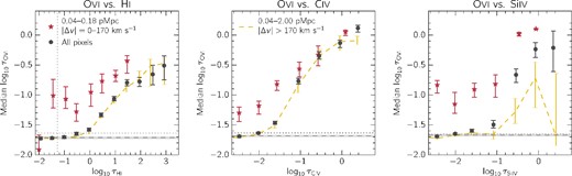
Left-hand panel: the O vi(H i) relation for the full sample of pixels (black circles) and for pixels located at small galactocentric distances (red stars). Error bars indicate the 1σ uncertainty determined by bootstrap resampling the galaxies. The median values for the full sample are denoted by the horizontal and vertical dotted black lines. The O vi flat level, defined as the median value for all O vi pixels that have associated |$\tau _{\rm H\, {\small I}}<\tau _{\rm H\, {\small I},{\rm cut}}=0.1$|, is represented by the horizontal dashed grey line, and the shaded region shows its 1σ error. The dashed line shows the optical depth relation for the full pixel sample after masking out regions within ±170 km s−1 of known galaxy redshifts, where we have considered galaxies with impact parameters of up to 2 pMpc. For a given H i optical depth, we find a strong enhancement for the median O vi optical depth for pixels at small galactocentric distances. Centre and right-hand panels: the same as the left-hand panel except for O vi(C iv) and O vi(Si iv). The fact that we observe the same trend when binning by different ions along the x-axis provides additional evidence that the effect we are seeing is real.
The median pixel optical depth values plotted in Fig. 1.
| All pixels | 0.04–0.18 pMpc | ||
|---|---|---|---|
| Δv = ±170 km s−1 | |||
| |$\log _{10} \tau _{\rm H\, {\small I}}$| | |$\log _{10} \tau _{\rm O\,\small {vi}}$| | |$\log _{10} \tau _{\rm H\, {\small I}}$| | |$\log _{10} \tau _{\rm O\,\small {vi}}$| |
| −1.94 | |$-1.73_{-0.02}^{+0.02}$| | −2.01 | |$-1.91_{-4.09}^{+0.24}$| |
| −1.49 | |$-1.72_{-0.02}^{+0.02}$| | −1.45 | |$-1.01_{-0.21}^{+0.27}$| |
| −1.02 | |$-1.70_{-0.02}^{+0.02}$| | −0.95 | |$-1.07_{-0.16}^{+0.21}$| |
| −0.53 | |$-1.65_{-0.03}^{+0.02}$| | −0.53 | |$-1.28_{-0.16}^{+0.13}$| |
| −0.04 | |$-1.58_{-0.03}^{+0.03}$| | 0.04 | |$-0.95_{-0.24}^{+0.14}$| |
| 0.44 | |$-1.33_{-0.03}^{+0.03}$| | 0.48 | |$-0.77_{-0.20}^{+0.12}$| |
| 0.96 | |$-1.07_{-0.04}^{+0.04}$| | 1.02 | |$-0.68_{-0.10}^{+0.09}$| |
| 1.47 | |$-0.80_{-0.06}^{+0.05}$| | 1.47 | |$-0.43_{-0.21}^{+0.09}$| |
| 1.96 | |$-0.78_{-0.08}^{+0.07}$| | ||
| 2.48 | |$-0.66_{-0.17}^{+0.15}$| | ||
| |$\log _{10} \tau _{\rm C\,\small {iv}}$| | |$\log _{10} \tau _{\rm O\,\small {vi}}$| | |$\log _{10} \tau _{\rm C\,\small {iv}}$| | |$\log _{10} \tau _{\rm O\,\small {vi}}$| |
| −2.47 | |$-1.69_{-0.02}^{+0.02}$| | −2.48 | |$-1.30_{-0.15}^{+0.10}$| |
| −2.01 | |$-1.64_{-0.02}^{+0.02}$| | −2.00 | |$-1.18_{-0.14}^{+0.08}$| |
| −1.61 | |$-1.46_{-0.03}^{+0.03}$| | −1.57 | |$-0.82_{-0.10}^{+0.06}$| |
| −1.05 | |$-0.77_{-0.05}^{+0.05}$| | −1.03 | |$-0.56_{-0.13}^{+0.11}$| |
| −0.55 | |$-0.35_{-0.05}^{+0.07}$| | −0.57 | |$-0.33_{-0.19}^{+0.15}$| |
| −0.05 | |$-0.13_{-0.08}^{+0.05}$| | 0.08 | |$0.05_{-0.06}^{+0.03}$| |
| 0.38 | |$0.12_{-0.07}^{+0.05}$| | ||
| |$\log _{10} \tau _{\rm Si\,\small {iv}}$| | |$\log _{10} \tau _{\rm O\,\small {vi}}$| | |$\log _{10} \tau _{\rm Si\,\small {iv}}$| | |$\log _{10} \tau _{\rm O\,\small {vi}}$| |
| −2.45 | |$-1.69_{-0.02}^{+0.02}$| | −2.44 | |$-0.83_{-0.13}^{+0.07}$| |
| −2.01 | |$-1.65_{-0.02}^{+0.02}$| | −2.02 | |$-1.15_{-0.16}^{+0.19}$| |
| −1.61 | |$-1.60_{-0.03}^{+0.03}$| | −1.55 | |$-0.91_{-0.13}^{+0.10}$| |
| −1.09 | |$-1.50_{-0.06}^{+0.07}$| | −1.04 | |$-0.82_{-0.22}^{+0.16}$| |
| −0.54 | |$-0.66_{-0.13}^{+0.10}$| | −0.47 | |$0.02_{-0.04}^{+0.03}$| |
| −0.07 | |$-0.24_{-0.14}^{+0.11}$| | −0.06 | |$0.10_{-0.01}^{+0.01}$| |
| 0.36 | |$-0.21_{-0.40}^{+0.28}$| | ||
Focusing on the black circles, there are two distinct regions in H i optical depth, separated by3|$\tau _{\rm H\, {\small I}, {\rm cut}}\sim 0.1$|. For |$\tau _{\rm H\, {\small I}}>\tau _{\rm H\, {\small I}, {\rm cut}}$|, |$\tau _{\rm O\,\small {vi}}$| increases with |$\tau _{\rm H\, {\small I}}$|. This relation arises because a large number of these pixel pairs are probing regions which have been enriched by oxygen, and the value at each pixel is set by the median number density ratio of O vi to H i.
For lower values of |$\tau _{\rm H\, {\small I}}$| (below |$\tau _{\rm H\, {\small I},{\rm cut}}$|), |$\tau _{\rm O\,\small {vi}}$| stays approximately constant, which indicates that the measured value is determined by residual contamination or noise and that the true, median value of |$\tau _{\rm O\,\small {vi}}$| is below this detection limit. In general, this asymptotic value of |$\tau _{\rm O\,\small {vi}}$| is slightly less than the median O vi optical depth of the full sample of pixels (the value is given in Table 1, and is indicated by the horizontal dotted black line in Fig. 1). We attempt to measure the constant value to which the O vi pixel optical depths asymptote, which we call the O vi flat level. As in Aguirre et al. (2008), we take this flat level to be the median of all |$\tau _{\rm O\,\small {vi}}$| pixels associated with |$\tau _{\rm H\, {\small I}} < \tau _{\rm H\, {\small I}, {\rm cut}}$|.
Furthermore, we estimate a 1σ error on this quantity by dividing each spectrum into 5 Å chunks and creating 1000 bootstrap resampled spectra. The flat level and the associated 1σ error are denoted by the black dashed line and grey region, respectively. It is difficult to probe O vi optical depths below the flat level, as one becomes limited by contamination. Specifically, absorption from ions with rest wavelength less than that of H i Lyα are found bluewards of the QSO Lyα emission line, and their recovery is limited by contamination from H i and other metal lines. These metal transitions are less affected by the quality (S/N) of the spectra and are more sensitive to the method of recovery. On the other hand, for ions redwards of the QSO's Lyα emission, the median pixel optical depths are set mainly by the S/N and/or shot noise, since the majority of pixels do not have detectable metal absorption. The two right-hand panels of figs 4 and 5 in Aguirre et al. (2002) show the changes on the median levels for different recovery methods and S/N ratios for O vi (bluewards of the QSO Lyα emission) and C iv (redwards of the QSO Lyα emission) using simulated spectra. These figures clearly demonstrate how the median level for O vi is more sensitive to recovery method while for C iv changing the S/N has a greater effect.
Turning next to the red stars in the left-hand panel of Fig. 1, we see a significant enhancement of |$\tau _{\rm O\,\small {vi}}$| at fixed |$\tau _{\rm H\, {\small I}}$| for the small galactocentric distance pixels compared to the full pixel sample. Such a difference is not present if we consider larger impact parameter bins (not shown). We emphasize that although the full pixel sample is representative of random regions, it is composed of pixels both near and far from galaxies (and many of these galaxies are likely not detected in our survey). To demonstrate this, we examine the effect of masking out the regions in the spectra that are known to be near galaxies. We consider all galaxies in our sample with impact parameters ≤2 pMpc and with redshifts satisfying equation (1), and mask out regions of ±170 km s−1 around these redshifts in all 15 of our QSO spectra. The resulting optical depth relation is shown as the dashed line in the left-hand panel of Fig. 1, and we conclude that the full pixel sample relation is largely independent of the presence of regions proximate to detected galaxies.
Next, we vary the ion plotted along the x-axis. In the centre and right-hand panels of Fig. 1, we show the relations for O vi(C iv) and O vi(Si iv), respectively (the values are also given in Table 2). Just as for O vi(H i), we observe significantly enhanced O vi optical depths at both fixed |$\tau _{\rm C\,\small {iv}}$| and fixed |$\tau _{\rm Si\,\small {iv}}$|. The persistent enhancement of O vi absorption at fixed optical depth of three distinct ions (H i, C iv, and Si iv) makes the individual detections with respect to each ion still more significant. Here we note that although the O vi(H i) and O vi(C iv) optical depth relations for which the galaxy positions have been masked out of the spectra show significant signal, this is not the case for O vi(Si iv). This suggests that strong Si iv absorption arises primarily near galaxies.
It is instructive to assess how sensitive the enhancement is to the chosen velocity range. We have examined the O vi(H i) relation for velocity bins starting with |Δv| = 0–170 km s−1 and increasing both velocity limits by increments of 10 km s−1 (such that each cut spanned the same total velocity range of 340 km s−1). We found that for optical depth bins with |$\tau _{\rm H\, {\small I}}\lesssim 1$|, the enhancement is present up to a velocity range of |Δv| = 270–440 km s−1, and we take the midpoint of this bin, ∼350 km s−1, as an upper limit to the extent of the O vi enhancement. In Fig. 2 we show the relation for the |Δv| = 270–440 km s−1 velocity bin (central panel), as well as higher and lower velocity cuts (right- and left-hand panels, respectively). For most of the optical depth bins with |$\tau _{\rm H\, {\small I}}>1$|, the enhancement in O vi is only significant for velocities within ±170 km s−1 of the galaxy positions.

The same as Fig. 1 but we have overplotted the result of taking different velocity cuts when considering the small galactocentric distance points (blue squares). We have chosen velocity bins such that each cut spans the same velocity range of 340 km s−1, and find that the enhancement of O vi at fixed |$\tau _{\rm H\, {\small I}}$| is present for |$\tau _{\rm H\, {\small I}}\lesssim 0.1$| out to the |Δv| = 270–440 km s−1 velocity cut. Using the central value of this velocity range as our upper limit, we conclude that the enhancement persists out to ∼350 km s−1, which is ≳1.5 times the typical circular velocities of the galaxies in our sample.
Although for the remainder of the analysis we will continue using the smallest velocity cut of |Δv| = 0–170 km s−1 we emphasize that for the lowest H i optical depth bins, O vi is enhanced out to velocities of ∼350 km s−1, corresponding to ≳1.5 times the typical circular velocities of the galaxies in our sample. While simulations predict that absorbers from galaxies below the detection limit can be projected to such velocities around their more massive counterparts (e.g. Rahmati & Schaye 2014), in Section 4 we determine that only a hot, collisionally ionized gas phase is observed out to these large velocities, which is certainly suggestive of outflows. Further comparisons with simulations will be required to fully disentangle outflow and clustering effects.
3.1 Are the observed differences in optical depth ratios real?
Fig. 1 suggests that the gas near the sample galaxies has properties different from that in random regions with the same strength of H i, C iv, or Si iv optical depth. However, it is important to verify that the difference between the two pixel samples is not driven primarily by chance or systematic errors. In particular, limiting ourselves to only a few regions of the spectra could skew the results if, for example, these regions have different S/N, or inconsistent contamination levels due to being located at different redshifts.
First, we would like to be sure that the enhancement in the median O vi optical depths is not due to a small number of pixels. In Fig. 3 we show the pixel optical depth probability density functions (PDFs) for H i, C iv, and Si iv, for both the small galactocentric distance and the full pixel samples (note that the x-axis ranges are larger than those shown in Fig. 1). Focusing on the small galactocentric distance pixels (red lines), one sees that the bins with enhanced median O vi (|$\log _{10} \tau _{\rm H\, {\small I}} \gtrsim -1$|; |$\log _{10} \tau _{\rm C\,\small {iv}}$| and |$\log _{10} \tau _{\rm Si\,\small {iv}} \gtrsim -2$|) comprise the majority of the pixels. Thus, the enhancement in the median O vi optical depth cannot be attributed to a small number of pixels.
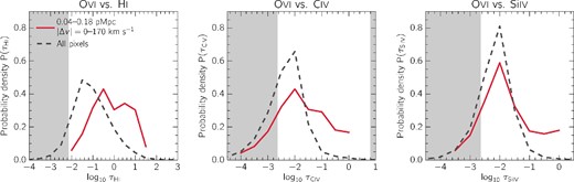
The probability density function of H i (left), C iv (centre), and Si iv (right) pixel optical depths for both the small galactocentric distance sample (red) and the full sample (black). For ease of comparison, we have shaded regions along the x-axis that are not included in the previous figures.
As a further test, in Fig. 4 we plot |$\tau _{\rm O\,\small {vi}}$| versus τX for the same τX shown in Fig. 1, but instead of using pixels within Δv = ±170 km s−1 of the galaxy redshifts, we look at regions further away, i.e. |Δv| = 2000–3000 km s−1. This velocity cut is near enough to the galaxy redshifts that within each impact parameter bin we are still looking at areas of the spectra with the same S/N and contamination characteristics, but far enough to avoid regions that may be associated with the galaxies. If the enhancement of the O vi optical depth at fixed H i, C iv, or Si iv that we detect near galaxies were caused by systematic differences in the spectral properties of the two samples, then we would expect to see the enhancement to a similar significance in these figures. However, in every case where we previously saw an enhancement in the median O vi optical depth for the pixels at small galactocentric distance, the effect is completely removed in Fig. 4.

The same as Fig. 1 but instead of taking pixels within ±170 km s−1 of the galaxy redshifts, the red stars show the effect of choosing regions within |Δv| = 2000–3000 km s−1 of the galaxy redshifts. By excluding the positions directly around the galaxies, but still using pixels within ∼103 km s−1 of the galaxy redshifts, we remove physical effects caused by the presence of the galaxy while probing the same spectral properties such as S/N, resolution, and distance from the QSO. Contrary to Fig. 1, the O vi absorption is not enhanced for the small galactocentric distance sample, which implies that the enhancement visible in that figure is not due to systematic differences in the spectral properties between the two samples.
Next, we examine whether the optical depth differences are consistent with random fluctuations. To do this, we take the galaxies from the small galactocentric distance sample, randomize their redshifts 1000 times, and calculate O vi(H i), O vi(C iv), and O vi(Si iv) for every random realization. In Fig. 5 we show the 1, 2, and 3σ percentiles that result from this procedure. From this, we measure the enhancements seen in O vi(H i), O vi(C iv), and O vi(Si iv) to be approximately a 2–3σ effect per bin.

The same as Fig. 1, except that we have overplotted the results of randomizing the redshifts of the small galactocentric distance galaxies 1000 times. For each of these randomizations, we recompute O vi(H i), O vi(C iv), and O vi(Si iv), and in this figure we show the median, the 84.1, 98.7, and 99.8 percentiles (corresponding to 0, 1, 2, and 3σ, respectively) from the full distribution of realizations. We find that the enhancement of O vi for fixed |$\tau _{\rm O\,\small {vi}}$|, |$\tau _{\rm C\,\small {iv}}$|, and |$\tau _{\rm Si\,\small {iv}}$| is approximately a 2–3σ effect per bin.
Additionally, because we do not observe differences in the O vi(H i), O vi(C iv), and O vi(Si iv) relations for galaxies with impact parameters >180 pkpc and the full pixel sample, here we check whether the O vi enhancement for the galaxies with impact parameters <180 pkpc can be attributed to properties other than the galaxy distance to the QSO sightline. We directly test whether the following three characteristics in every impact parameter bins are consistent with the full sample: (1) the galaxy redshifts (lower galaxy redshifts mean that O vi is more contaminated by H i); (2) the galaxy velocity distance from the QSO Lyα emission (to rule out QSO proximity effects); and (3) the S/N of the spectral regions (smaller S/N will bias the optical depth estimation high).
We have measured the p-values resulting from a two-sample Kolmogorov–Smirnoff test, comparing the galaxy redshift, median S/N within ±170 km s−1 from the redshift of the galaxy, and redshift difference between the galaxy and the QSO, between the galaxies in the small galactocentric distance sample and the full galaxy sample. In every instance we find p-values greater than 0.1, which is consistent with the null hypothesis that the two samples are drawn from the same distribution.
Finally, in Appendix A we have tested how the O vi contamination correction affects our results. We determined that although the inferred values of the O vi optical depths are sensitive to changes in the correction procedure, the enhancement of O vi optical depths at fixed H i the O vi for pixels at small galactocentric distances compared to random regions is unchanged, and remains significant irrespective of the contamination correction details. Thus, we conclude that the observed optical depth differences are neither due to chance nor to systematic variations in the spectral characteristics in either the QSOs or the galaxies.
4 IONIZATION MODELS
In this section, we will investigate the physical origin of the difference in O vi observed between regions near our galaxies and in random locations. We focus on O vi(H i) because binning by |$\tau _{\rm H\, {\small I}}$| enables a more straightforward physical interpretation than binning by metal ion optical depth, due to the tight correlation between H i absorption and gas density in photoionized gas. We consider three possible scenarios and examine their plausibilities. The first hypothesis we consider is enriched photoionized (T ∼ 104 K) gas, where the enhanced O vi(H i) near galaxies might be explained by higher gas metallicities. Second, we test the idea that ionizing radiation from the nearby galaxy could be responsible for the increase in O vi(H i). Finally, we consider whether our observations can be explained by a hot, collisionally ionized enriched gas phase near galaxies. We argue that of these three, the first scenario (enriched photoionized gas) can account for pixels with |$\tau _{\rm H\, {\small I}}\gtrsim 10$|, while only the third explanation (the presence of hot, enriched gas) is plausible for pixels with |$\tau _{\rm H\, {\small I}}\lesssim 1$|. Of course, it is important to note that every H i bin likely contains a mixture of pixels from different gas phases and ionization sources; the final behaviour is simply determined by the dominant phase.
4.1 Photoionization by the background radiation
The optical depth of H i is believed to be a good tracer of the photoionized gas density, even on an individual pixel basis (Aguirre et al. 2002). Hence, if the gas probed were predominantly photoionized and if the abundance of oxygen depended only on gas density, we would not expect to see any difference between the O vi(H i) relations of all pixels and those known to lie near galaxies in Fig. 1. Since a clear difference is observed, we postulate that this could be caused by an increase in the oxygen abundance near galaxies at fixed gas densities.
To test this idea, we turn to ionization modelling using cloudy (version 13.03; Ferland et al. 2013). Our set-up involves a plane-parallel slab illuminated uniformly by an ionizing background, along a grid of varying temperatures and hydrogen densities, that covers both photoionization equilibrium (PIE) and collisional ionization equilibrium (CIE, discussed in Section 4.3). For the fiducial case we use the ionizing background from Haardt & Madau (2001) including contributions from both quasars and galaxies, normalized to match the z = 2.34 metagalactic H i photoionization rate, Γ = 0.74 × 10⁻¹² s−1, from Becker, Rauch & Sargent (2007).4 However, the shape and normalization of the background are subject to large uncertainties, and we explore the effect of varying them in Appendix C.5
![Theoretical optical depth ratios ($\log _{10} \tau _{\rm O\,\small {vi}} / \tau _{\rm H\, {\small I}}$) as a function of temperature and hydrogen density from cloudy modelling. For this figure we have assumed [O/H] = 0.0, however, we allow this value to vary according to equation (3) when comparing with the observations. The vertical dashed line denotes T = 2 × 10⁴ K, which is the temperature that we assume in the case of PIE. Furthermore, under the assumption of PIE we can convert hydrogen number densities to H i optical depths with equation (5), and we show corresponding $\tau _{\rm H\, {\small I}}$ values on the right-hand y-axis. For CIE, we can use the ratios to set lower limits on the metallicity by using the maximum ratio from this temperature–density plane. This maximum occurs at T = 3 × 10⁵ K and is marked by the small black circle at nH = −2.](https://oup.silverchair-cdn.com/oup/backfile/Content_public/Journal/mnras/450/2/10.1093/mnras/stv750/2/m_stv750fig6.jpeg?Expires=1750525765&Signature=eHPVYvjwG8GZRlDBn6urZBjGDXPHjbM7xKNxCaM-O6Awipvzd5YiFudc8xpdmeEgDKvTZGT2rSSzBW3ZuuE6B3Bl39ZUxzaaOC3udFK2uuoDSm4pP5feYXoz7Qz2-3S9bvkUasL8ZPbPK~HLuFbBE673lxBR44GXkFq3vkHsfBpEtb43WBvMJqbjAygt-sFtZ4ASHCxsVlFlIv9JT-lL3VJHYwUOzFs1Wpt6lzGAnoPctT4C5JnshuZ1KrXnz19hUv9xSJ7Eu37CzEAYnMIy~GTg8GTAFPd8xWI4oUk~DEWDBDDty5Caf2ZhuxYkYqothV-8~wMVnN5~2yS~fHxHsg__&Key-Pair-Id=APKAIE5G5CRDK6RD3PGA)
Theoretical optical depth ratios (|$\log _{10} \tau _{\rm O\,\small {vi}} / \tau _{\rm H\, {\small I}}$|) as a function of temperature and hydrogen density from cloudy modelling. For this figure we have assumed [O/H] = 0.0, however, we allow this value to vary according to equation (3) when comparing with the observations. The vertical dashed line denotes T = 2 × 10⁴ K, which is the temperature that we assume in the case of PIE. Furthermore, under the assumption of PIE we can convert hydrogen number densities to H i optical depths with equation (5), and we show corresponding |$\tau _{\rm H\, {\small I}}$| values on the right-hand y-axis. For CIE, we can use the ratios to set lower limits on the metallicity by using the maximum ratio from this temperature–density plane. This maximum occurs at T = 3 × 10⁵ K and is marked by the small black circle at nH = −2.
Solar abundances used in this work, taken from cloudy 13.
| Element | ni/nH | Ref. |
|---|---|---|
| H | 1 | |
| C | 2.45 × 10⁻⁴ | 1 |
| O | 4.90 × 10⁻⁴ | 2 |
| Si | 3.47 × 10⁻⁵ | 3 |
| Element | ni/nH | Ref. |
|---|---|---|
| H | 1 | |
| C | 2.45 × 10⁻⁴ | 1 |
| O | 4.90 × 10⁻⁴ | 2 |
| Si | 3.47 × 10⁻⁵ | 3 |
We would like to compare the observed optical depth ratios with those predicted from cloudy in order to estimate the gas metallicity. To compute the observed ratios, we begin with the |$\tau _{\rm O\,\small {vi}}$| points in the left-hand panel Fig. 1. In order to correct for the presence of residual contamination from absorption by species other than O vi, we subtract the flat level (i.e. the asymptotic value of |$\tau _{\rm O\,\small {vi}}$| reached for small |$\tau _{\rm H\, {\small I}}$| and indicated by the horizontal, dashed line in Fig. 1) from all |$\tau _{\rm O\,\small {vi}}$| values. Following Schaye et al. (2003), to be conservative we added the error on the flat level linearly (rather than in quadrature) to the errors on |$\tau _{\rm O\,\small {vi}}$|, and finally we divide every |$\tau _{\rm O\,\small {vi}}$| point by its corresponding |$\tau _{\rm H\, {\small I}}$|. The results of this calculation are plotted in the left-hand panel Fig. 7.
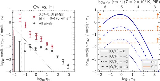
Left-hand panel: the ratio of O vi to H i optical depths as a function of |$\tau _{\rm H\, {\small I}}$|. To compute these points, we used the data from Fig. 1. First, we subtracted the O vi flat level from the median O vi optical depths, in order to correct for contamination. After dividing the resulting values by their corresponding H i optical depths, we obtain the points plotted here. The black vertical dotted line corresponds to the median value of all H i pixel optical depths, while the diagonal line shows the median value of all O vi pixel optical depths divided by the given value of |$\tau _{\rm H\, {\small I}}$| along the x-axis. Right-hand panel: theoretical ratios of O vi to H i as a function of |$\tau _{\rm H\, {\small I}}$| taken from cloudy modelling (see Fig. 6). First, in the case of PIE, we assume that the gas has a temperature of 2 × 10⁴ K, and convert H i optical depths to a hydrogen number density using equation (5) (the corresponding nH values are shown on the upper y-axis). The blue curves show profiles taken along the vertical black dashed line in Fig. 6, where the different line styles demonstrate the effect of varying the metallicity. We also consider CIE, in which case cannot estimate the density from |$\tau _{\rm H\, {\small I}}$|. Instead, we can use the maximum theoretical ratio (indicated by the black circle at T = 3 × 10⁵ in Fig. 6) to set a lower limit on the metallicity, and these are shown by the horizontal orange lines.
Thus, we can use equation (5) to convert between H i optical depth and hydrogen number density. Next, we consider the contour along a constant temperature of T = 2 × 10⁴ K in Fig. 6, from which we obtain theoretical optical depth ratios as a function of nH. With equation (5), we can convert the nH dependence to corresponding values of |$\tau _{\rm H\, {\small I}}$|. The result of doing so is shown by the blue lines in Fig. 6, where the different line styles demonstrate the effect of varying the metallicity using equation (3).
Hence, by interpolating between the blue curves in the right-hand panel of Fig. 7, we can estimate a metallicity (assuming PIE) for each optical depth ratio |$\tau _{\rm O\,\small {vi}}/\tau _{\rm H\, {\small I}}$| in the left-hand panel. The outcome of this procedure is plotted in the left-hand panel of Fig. 8. To aid the interpretation, we indicate the baryon overdensity inferred from |$\tau _{\rm H\, {\small I}}$| along the upper x-axis (again, we can only convert H i optical depth to overdensity under the assumption of PIE).
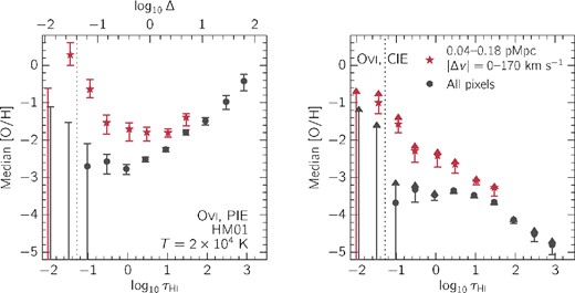
Left-hand panel: metallicity as a function of H i pixel optical depth. The metallicity was inferred from the ratio of |$\tau _{\rm O\,\small {vi}}$| to |$\tau _{\rm H\, {\small I}}$| (Fig. 7) assuming PIE (T = 2 × 10⁴ K) as described in the text. On the upper axis we show |$\tau _{\rm H\, {\small I}}$| converted to an overdensity Δ using the relation for photoionized gas that we assumed in the ionization models. Random regions (black circles) show a positive correlation between metallicity and density, while at small galactocentric distances (red stars) for |$\tau _{\rm H\, {\small I}}\lesssim 1$| the metallicity increases inversely with density. Such an inverted metallicity–density relation is not physically expected and indicates that the assumption of PIE is probably incorrect. Right-hand panel: lower limits on the metallicity as a function |$\tau _{\rm H\, {\small I}}$|, inferred again from the measured optical depth ratios but now assuming CIE. The size of each arrow is proportional to the size of the error bar on the measured optical depth ratio. The inferred limits on the metallicity are lower than for PIE, but still imply that at least some of the gas near galaxies is substantially enriched.
Focusing first on the black points that correspond to the full pixel sample, we find that metallicity increases with overdensity Δ, and is in agreement with previous pixel optical depth studies (e.g. Schaye et al. 2003; Aguirre et al. 2008). Next, examining the values derived from pixels with small galactocentric distance (red stars), for pixels with |$\tau _{\rm H\, {\small I}}\gtrsim 10$| we infer the same metallicity–density relation as for the full pixel sample, but with metallicities that are ∼0.5 dex higher. We conclude that for these H i optical depths, photoionized gas that is enriched with respect to random regions of the same density is consistent with our observations of O vi(H i) at small galactocentric distances.
However, turning to pixels with |$\tau _{\rm H\, {\small I}}\lesssim 1$|, it is clear that the relation between metallicity and density is inverted. In this regime, the metallicity appears to increase with decreasing overdensity, with the highest metallicities found at the lowest overdensities, even reaching supersolar values. We do not consider this enrichment pattern to be physically plausible. Although some regions of relatively low density can be highly enriched, they usually arise in hot superbubbles. Furthermore, an underdense gas phase close to galaxies with T ∼ 104 K and supersolar metallicities is not consistent with predictions from cosmological hydrodynamical simulations (e.g. Ford et al. 2013; Shen et al. 2013). The above suggests that one or more of our assumptions must be incorrect for the small galactocentric distance pixel sample.
4.2 Photoionization by stars in nearby galaxies
In this section, we test whether the enhancement of |$\tau _{\rm O\,\small {vi}}$| for a fixed |$\tau _{\rm H\, {\small I}}$| near galaxies can be explained by increased photoionization by radiation from the stars in the nearby galaxies. At sufficiently small galactocentric distances, we would expect the mean hydrogen ionization rate to be dominated by galactic radiation rather than by the metagalactic background radiation (e.g. Schaye 2006; Rahmati et al. 2013), which would reduce the H i optical depth at fixed density. Furthermore, since stars emit very little radiation with photon energies >4 Ryd, we do not expect the O vi optical depth to be modified by local stellar sources, given that the ionization energy for O v is about 8.4 Ryd. Hence, if photoionization by nearby galaxies were important, we would expect the red stars in Fig. 1 to be shifted upwards relative to the black points and the red stars in Fig. 7 to be shifted towards the top-left relative to the black points. This is qualitatively consistent with the observations, which suggests that the difference between the two samples may be due to photoionization by local sources rather than due to the presence of hot, enriched gas. However, as we will show below, quantitatively this scenario does not work out.
The remaining unknown in our estimate of the photoionization rate from local galaxies comes from the ratio of the escape fractions at 1 Ryd and at the observed wavelength of 1700 Å, fesc, λ912/fesc, λ1700. The literature contains many values for the escape fraction of Lyman continuum photons relative to that of non-ionizing UV continuum photons, fesc,rel ≡ fesc,λ900/fesc,λ1500. Values range from ∼1 to 83 per cent (e.g. Steidel, Pettini & Adelberger 2001; Shapley et al. 2006; Iwata et al. 2009; Mostardi et al. 2013; Nestor et al. 2013; Cooke et al. 2014), although typical values are closer to the lower limit of this range.
Since we already expect |$\Gamma _{\nu _0} = 0.74 \times 10^{-12}$| s−1 from the extragalactic background (Becker et al. 2007), adding a contribution from nearby galaxies would boost the H i photoionization rate by a factor of ∼20 for an escape fraction fesc,rel = 100 per cent at the median impact parameter and would hence suppress the H i optical depths by the same amount. To test whether ionizing radiation from nearby galaxies can explain the difference between the O vi(H i) relations of the small galactocentric radii and the random pixel samples, we have re-calculated the O vi(H i) relation for random regions after dividing all the H i pixel optical depths by the factor by which local sources boost the H i ionization rate for various values of the relative escape fraction. The results are compared with the observed relation for the small galactocentric radii sample in Fig. 9. For fesc,rel ≤ 10 per cent the effect of local sources is not strong enough to reproduce the observations. Even for the highly unrealistic case that fesc,rel = 100 per cent, the boost in the H i ionization rate is insufficient to completely account for the observed enhancement of O vi small galactocentric distances for |$\tau _{\rm H\, {\small I}}\lesssim 1$|.

The data points are identical to those in the left-hand panel of Fig. 1. The curves show the result for the full pixel sample (black circles) after dividing the H i optical depths by the boost factor in the H i photoionization rate expected due to ionizing radiation from the nearby galaxy for the relative escape fractions, fesc,rel ≡ fesc,λ900/fesc,λ1500, indicated in the legend and for a distance to the source equal to the median impact parameter of the pixels in the small galactocentric distance sample. Even for fesc,rel = 100 per cent, which is unrealistically high, the curve falls short of the red stars, implying that photoionization by radiation from the observed galaxies cannot explain the observed enhancement in O vi/H i near galaxies.
On the other hand, while for |$\tau _{\rm H\, {\small I}}\gtrsim 10$| it appears that relative escape fractions of ∼50 per cent may be able to explain our observations, we reiterate that average observed relative escape fraction values are usually much lower than this for galaxies such as ours (e.g. Shapley et al. 2006). Furthermore, we note that by considering only the transverse rather than three-dimensional distance to the galaxy, our estimate of the H i photoionization rate boost is strictly an upper limit, and the true strength of the effect is almost certainly smaller.
As a final test, we have taken the blackbody spectrum used to approximate the local galaxy radiation and used it as input, along with the extragalactic background, into cloudy. We generated temperature–density planes showing optical depth ratios |$\tau _{\rm O\,\small {vi}}/\tau _{\rm H\, {\small I}}$| (as in the right-hand panel of Fig. 7), as well as |$\tau _{\rm O\,\small {vi}}/\tau _{\rm C\,\small {iv}}$| and |$\tau _{\rm O\,\small {vi}}/\tau _{\rm Si\,\small {iv}}$|, and compared these with the output using only the extragalactic background. For the O vi(H i) relation, we indeed found that the predicted ratios for photoionized gas at ∼104 K were higher. However, as expected due to the fact that our assumed spectrum does not contain many photons with energies above 1 Ryd, for the observed ratio values there was almost no discernible difference between the O vi(C iv) and O vi(Si iv) relations derived with and without the contribution from nearby galaxies.6 Hence, if local sources were responsible for the enhancement in O vi(H i), we would not expect to see any difference between the small galactocentric distance and random pixel samples for the O vi(C iv) and O vi(Si iv) relations. This is not consistent with the fact that we find significantly enhanced O vi for both fixed C iv and fixed Si iv much like we do for the O vi(H i) relation (see the centre and right-hand panels of Fig. 1). Thus, we conclude that enhanced photoionization due to the proximity of the observed galaxies cannot explain the enhancement of O vi at fixed H i that we observe for the small galactocentric distance pixel sample.
In the above scenario, we only consider photoionization by stars in the nearby galaxies because there is no evidence that our galaxies contain AGN. However, it was recently pointed out by Oppenheimer & Schaye (2013b) that because of the long recombination times for metals at densities typical of the circumgalactic medium, ions like O vi may remain out of ionization equilibrium long after the AGN episode is over. In fact, for reasonable AGN duty cycles, the authors argue that much of the O vi detected in quasar spectra resides in such fossil AGN proximity zones. On the other hand, in regions where the equilibrium neutral hydrogen fraction is low, H i will equilibrate nearly instantaneously after the AGN turns off. Hence, in this scenario H i would be photoionized and in equilibrium, while O vi is out of equilibrium and enhanced because of the fossil AGN proximity effect. We would then expect the enhancement in O vi to be strongest in regions of low H i absorption, since such regions correspond to low densities and thus long recombination times. This is in qualitative agreement with our observations, although Oppenheimer & Schaye (2013b) show that at very low density oxygen will become so highly ionized that O vi is suppressed, which would be inconsistent with our findings.
More generally, since (fossil) AGN proximity and higher gas temperatures both tend to increase the abundance of more highly ionized species relative to ions with lower ionization potentials, many of the predictions of these two scenarios will be qualitatively similar, although it remains to be seen whether the fossil proximity effect can work quantitatively. One important difference, however, is the expected widths of the absorption lines. If the oxygen is hot enough for O vi to be collisionally ionized, then the absorption lines will be broader than if the gas were photoionized. We intend to measure the widths of the metal absorption lines and to model the fossil AGN proximity effect in future work.
4.3 Collisionally ionized gas
It may be that at small galactocentric distances, much of the O vi absorption arises in collisionally ionized rather than photoionized gas. Indeed, the behaviour of the O vi(H i) relation for the near-galaxy pixels with |$\tau _{\rm H\, {\small I}}\lesssim 1$| points to collisional ionization playing a role. In general, we would not expect to see very much H i associated with collisionally ionized O vi, as the H i fraction is very low at T > 105 K. The behaviour of the [O/H](Δ) relation that we inferred under the assumption of photoionization (Fig. 8) is rather suggestive, as the relation displays larger departures from the random regions with decreasing |$\tau _{\rm H\, {\small I}}$|.
If we are in fact probing collisionally ionized gas, then we cannot measure its metallicity as was done in Section 4.1 – first because we are unable to estimate the gas density from the H i optical depth, and second because there is no natural equilibrium temperature. However, it is possible to put a lower limit on the metallicity by selecting the temperature and density that would maximize |$\tau _{\rm O\,\small {vi}}/\tau _{\rm H\, {\small I}}$|. In Fig. 6, we have marked the temperature and density where this theoretical maximum is reached by a small black circle. Then, in the right-hand panel of Fig. 7, the horizontal orange lines show the |$\tau _{\rm O\,\small {vi}}/\tau _{\rm H\, {\small I}}$| ratio at this point for different metallicities.
Thus, irrespective of H i optical depth (which has no correspondence with density under the assumption of CIE) we can convert the observed optical depth ratios in the left-hand panel of Fig. 7 to lower limits on the metallicity, and we show the result in the right-hand panel of Fig. 8. As expected, the limits obtained are lower than the metallicities inferred when assuming photoionization. Nevertheless, some of the lower limits are sufficiently high to be interesting. The 1σ lower limit approaches [O/H] ∼ −1 at the lowest bins in H i optical depth, where |$\log _{10}\tau _{\rm H\, {\small I}}=-1.5$|.
Given the reasonable metallicity limits in Fig. 8 combined with the fact that the previous two scenarios (photoionization by the extragalactic background or by local stellar radiation) cannot account for the O vi enhancement for |$\tau _{\rm H\, {\small I}}\lesssim 1$|, we conclude that collisional ionization is the dominant ionization source for a significant fraction of the small galactocentric distance pixels. We emphasize that in collisionally ionized gas, |$\tau _{\rm H\, {\small I}}$| is no longer a good estimator of density, and we could potentially be probing very high overdensities.
We also examined the O vi/C iv and O vi/Si iv ratios in Appendix B. We conclude that O vi pixels near galaxies are more consistent with a hotter gas phase than the full pixel sample, and furthermore we find that the strength of this trend increases inversely with C iv and Si iv optical depths, as might be expected for collisionally ionized gas at ∼3 × 10⁵ K where these other ions are not abundant. However, since the results are not constraining, the details are left to the appendices.
5 DISCUSSION AND CONCLUSIONS
We have used absorption by H i and metals to study the physical conditions near z ∼ 2.3 star-forming galaxies in the fields of 15 hyperluminous background QSOs that have been observed with Keck/HIRES as part of the KBSS. We focused on 21 galaxies with impact parameters <180 pkpc and isolated the pixels of the quasar spectra that are within ±170 km s−1 of the accurate galaxy redshifts provided by the KBSS. In Turner et al. (2014) we showed that the absorption by H i and various metal ions is strongly enhanced in these circumgalactic regions. The fact that both H i and the metals are enhanced raises the question whether the observed increase in the metal absorption merely reflects the presence of higher gas densities near galaxies or whether it implies that the gas near galaxies has a higher metallicity at fixed density or a different temperature from gas in random regions.
To address this question, we measured the pixel optical depths of O vi as a function of H i, C iv, and Si iv, and compared the results for the pixels located at small galactocentric distances to the full pixel sample, which is representative of random regions. Our main result is the detection of a 0.3–0.7 dex enhancement (which reaches its maximum at |$\log _{10} \tau _{\rm H\, {\small I}}\sim -1.5$|) in the median optical depth of O vi at fixed |$\tau _{\rm H\, {\small I}}$| for the small galactocentric distance sample when compared with the full pixel sample (Fig. 1). We verified that this enhancement, which we detected at 2–3σ confidence per logarithmic bin for |$\tau _{\rm H\, {\small I}}$|, |$\tau _{\rm C\,\small {iv}}$|, and |$\tau _{\rm Si\,\small {iv}}$|, is not due to differences in the redshift distribution or the quality of the quasar spectra between the small galactocentric distance and full pixel samples.
We proposed and tested three different hypotheses that may explain the observed enhancement of O vi(H i) near galaxies: (1) the gas is photoionized by the extragalactic background but has a higher metallicity at fixed density; (2) the gas is more highly ionized at fixed density by radiation from stars in the nearby galaxy; and (3) the enriched gas is hot and collisionally ionized.
To test scenario (1), we used cloudy ionization models and the relation between |$\tau _{\rm H\, {\small I}}$| and density for photoionized, self-gravitating clouds from Schaye (2001) and Rakic et al. (2012) to convert the observed optical depth ratios into a metallicity–density relation, assuming T ∼ 104 K, as expected for photoionized gas. We found that the full pixel sample gave a physically plausible metallicity–density relation that is consistent with previous studies which did not have information on the locations of galaxies. Furthermore, the same metallicity–density relation (but shifted up by ∼0.5 dex in metallicity) is also present for small galactocentric distance pixels that have |$\tau _{\rm H\, {\small I}}\gtrsim 10$|. Thus, for high H i optical depths, the enhancement of O vi at fixed |$\tau _{\rm H\, {\small I}}$| is consistent with arising predominantly from enriched, photoionized gas. However, making this same assumption of PIE for |$\tau _{\rm H\, {\small I}}\lesssim 1$| resulted in an [O/H] versus overdensity relation that cannot be easily explained, as [O/H] was found to increase strongly with decreasing overdensity, implying supersolar metallicities for underdense gas (left-hand panel of Fig. 8). We therefore concluded that while photoionization by the background radiation is a plausible scenario for the random regions, it cannot account for the observed enhancement of O vi(H i) near galaxies.
In scenario (2) O vi is enhanced at fixed H i because radiation from stars in the nearby galaxy suppresses H i, while leaving O vi unchanged. To test this explanation, we estimated the H i photoionization rate due to the galaxies. However, we found that only under the unrealistic assumptions that the relative escape fraction fesc,λ900/fesc,λ1500 is 100 per cent and that the 3D distance between the gas and the galaxy is equal to the impact parameter, can the flux of ionizing radiation from the galaxies explain the observed increase in |$\tau _{\rm O\,\small {vi}}/\tau _{\rm H\, {\small I}}$| near galaxies. Reducing the relative escape fraction to a still conservative value of 10 per cent rules out this scenario as a dominant ionization source (Fig. 9). Furthermore, we found that such a galaxy proximity effect is predicted to have a much smaller effect on O vi(C iv) and O vi(Si iv) than on O vi(H i), which is inconsistent with our observations.
Contrary to photoionization by either the extragalactic background or local stellar radiation, scenario (3) can explain the enhancement in O vi(H i) near galaxies for pixels with |$\tau _{\rm H\, {\small I}}\lesssim 1$|. If a substantial fraction of the enriched gas near galaxies is sufficiently hot for O vi to be collisionally ionized, i.e. T > 105 K, then we can account for the observations. By assuming the maximum O vi/H i ratio reached in CIE, we converted the observed optical depth ratios into lower limits on the metallicity, finding [O/H] ≳ −1 for gas with weak H i absorption (right-hand panel of Fig. 8). Indeed, this measurement is supported by other characterizations of KBSS galaxy properties. Rudie et al. (2012a) found higher temperatures for fixed |$\tau _{\rm H\, {\small I}}$| near the KBSS galaxies, while Steidel et al. (2014) measured H ii region metallicities of 0.4 Z⊙, which could serve as a possible upper limit to the value presented here (although if metal-enriched winds drive most of the metals out of the star-forming regions, it is possible that the circumgalactic gas may have a higher metallicity than galactic H ii regions). Furthermore, the inferred metallicities and temperatures of T ≳ 105 K are in agreement with the predictions of van de Voort & Schaye (2012) for galaxies with the masses and redshifts similar to ours.
In summary, we favour the conclusion that our galaxies are surrounded by hot (T > 105 K) gas of which a substantial fraction must have metallicity ≳10−1 of solar. Furthermore, we find that this metal-enriched phase extends out to ∼350 km s−1 of the galaxy positions (Fig. 2), which corresponds to ≳1.5 times the halo circular velocities. Because of the relatively high temperature that requires shock heating, the large velocity range extending far outside the haloes, and high metallicity, we conclude that we have detected hot, metal-enriched outflowing gas. Future comparisons with hydrodynamical simulations, considering ion ratios as well as the kinematics and line widths, will provide strong constraints on models of galaxy formation and may provide further insight into the interpretation of our observations.
We are very grateful to Milan Bogosavljevic, Alice Shapley, Dawn Erb, Naveen Reddy, Max Pettini, Ryan Trainor, and David Law for their invaluable contributions to the Keck Baryonic Structure Survey, without which the results presented here would have not been possible. We also thank Ryan Cooke for his help with the continuum fitting of QSO spectra. We gratefully acknowledge support from Marie Curie Training Network CosmoComp (PITN-GA-2009- 238356) and the European Research Council under the European Union's Seventh Framework Programme (FP7/2007-2013)/ERC Grant agreement 278594-GasAroundGalaxies. CCS, GCR, ALS acknowledge support from grants AST-0908805 and AST-13131472 from the US National Science Foundation. This work is based on data obtained at the W. M. Keck Observatory, which is operated as a scientific partnership among the California Institute of Technology, the University of California, and NASA, and was made possible by the generous financial support of the W. M. Keck Foundation. We thank the W. M. Keck Observatory staff for their assistance with the observations. We also thank the Hawaiian people, as without their hospitality the observations presented here would have not been possible.
Although this work does not use direct galaxy detections, the authors inferred that their strongest absorber sample probes regions defined as circumgalactic in Rudie et al. (2012a) in ≈60 per cent of cases. This was determined by using high-resolution quasi-stellar object (QSO) spectra from fields where the redshifts of Lyman-break galaxies with impact parameters <300 kpc are already known. The QSO spectra were degraded to match the resolution of the spectra used in Pieri et al. (2014), and a correction for the expected volume density of Lyman-break galaxies from Reddy et al. (2008) was applied.
As noted in Aguirre et al. (2008), because the O vi pixel relations are not as strong as for C iv, we fix the value of τcut by hand rather than using functional fits. We use the same values as in Aguirre et al. (2008) of τcut = 0.1 when pixel pairs are binned based on the optical depths of transitions that fall blueward of the QSO's Lyα emission (O vi, H i) and 0.01 for those falling redward (C iv, Si iv).
Measurements of Γ at z = 2.4 vary between Γ = 0.5 × 10⁻¹² s−1 in Faucher-Giguère et al. (2008) up to |$\Gamma = 1.0 \pm ^{0.40}_{0.26} \times 10^{-12}\,{\rm s}^{-1}$| in Becker & Bolton (2013). We choose the intermediate value of 0.74 × 10⁻¹² s−1 at z = 2.34 taken from the fitting formulas of Becker et al. (2007).
We note that the assumption of PIE may break down as non-equilibrium effects become important in cooling gas at temperatures <106 K. The presence of these effects causes collisional ionization to occur at lower temperatures compared to in equilibrium, although once an extragalactic background is included the impact of the effect of non-equilibrium cooling becomes less important (Oppenheimer & Schaye 2013a).
Invoking galaxy spectra with a soft X-ray component could potentially lead to more oxygen ionized to O vi (e.g. Cantalupo 2010), however, these spectral models remain uncertain and we leave testing of this scenario to a future work.
REFERENCES
APPENDIX A: CORRECTION OF O |$\small {vi}$| CONTAMINATION
Here we examine how modifying the O vi contamination correction affects the resulting O vi(H i) relation. It is possible that the small galactocentric distance pixel sample suffers from more H i contamination than the full pixel sample, given the larger on average H i optical depth values (see the left-hand panel of Fig. 3) and the proximity of Lyβ to O vi (∼1800 km s−1). We postulate that if the enhancement of O vi for fixed H i optical depths at small galactocentric distances were largely due to uncorrected H i Lyβ contamination, modification of the O vi contamination would have a notable effect on this enhancement.
To test this, in Fig. A1 we show the O vi(H i) relation as in the left-hand panel of Fig. 1, but with changes to the O vi contamination correction. In the fiducial case, we subtract five orders of the Lyman series of H i beginning with Lyβ, and then take the minimum of the O vi doublet optical depths. In Fig. A1, we first show O vi(H i) after not subtracting any H i but still taking the doublet minimum (left-hand panel), not taking the doublet minimum but still subtracting H i (centre panel), and not performing any correction at all (right-hand panel). Although the absolute values of the apparent O vi optical depths increase when fewer contamination corrections are performed, the significance of O vi optical depth at fixed H i for pixels at small galactocentric distance compared to the full pixel sample remains unchanged, indicating that our results are not sensitive to the O vi contamination correction procedure.
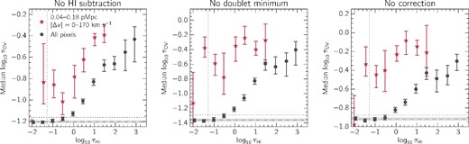
The same as the left-hand panel of Fig. 1, but varying the method of O vi contamination correction. The modifications shown here are the result of not subtracting any H i (left-hand panel), not taking the doublet minimum (centre panel), and not performing any correction at all (right-hand panel). This figure demonstrates that the qualitative behaviour of the enhancement of O vi optical depth at fixed H i for pixels at small galactocentric distance is entirely independent of the O vi contamination correction procedure.
Finally, we perform a simple calculation to demonstrate that the H i Lyβ contamination is not predicted to have a large effect. To begin, we would like to estimate the typical Lyβ strength at a distance ∼1800 km s−1 away from galaxies. For this, we use our measurement of the median optical depth as a function of distance along the galaxy LOS, as was done in the right-hand panels of fig. 6 from Turner et al. (2014), but extending out to ∼1800 km s−1. We find that the H i Lyα optical depths asymptote to the median value of all pixels (0.051), and using the relative oscillator strengths of Lyα and Lyβ we can convert this to an expected median value of H i Lyβ (0.0082). Adding this to the median value of all O vi pixels (0.023), we obtain 0.031. This corresponds to ∼− 1 in the left-hand panel of Fig. 1, and is significantly less than the observed O vi optical depth enhancement.
APPENDIX B: O |$\small {vi}$|(C |$\small {iv}$|) AND O |$\small {vi}$|(Si |$\small {iv}$|)
In the centre and right-hand panels of Fig. 1, we investigated whether the O vi(C iv) and O vi(Si iv) relations depend on galactocentric distance. First, we note that we see similar behaviour for O vi(C iv) and O vi(Si iv) as for O vi(H i) – that is, we find a higher |$\tau _{\rm O\,\small {vi}}$| at fixed τX for pixels near galaxies compared to random locations, and the magnitude of this enhancement increases with decreasing τX.
As in Section 3, we can use cloudy to model the optical depth ratios as a function of temperature and density. These temperature–density planes, along with the observed ratios, are shown in Fig. B1. We note that if we assume solar relative abundances, then the optical depth ratios determined from the cloudy models are fixed and do not depend on metallicity (unlike for optical depth ratios with |$\tau _{\rm H\, {\small I}}$| in the denominator).
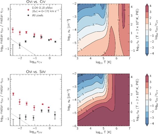
Left-hand column: median optical depth ratios derived from the O vi(C iv) (top) and O vi(Si iv) (bottom) relations in Fig. 1. The diagonal lines show the median value of all O vi pixel optical depths divided by the given value of |$\tau _{\rm C\,\small {iv}}$| and |$\tau _{\rm Si\,\small {iv}}$| along the x-axis, and demarcates a conservative detection level. Right-hand column: predicted optical depth ratios from cloudy.
Looking first at O vi(C iv), for |$\log _{10}\tau _{\rm C\,\small {iv}}\gtrsim -1$| pixels near galaxies and at random locations have similar optical depth ratios ranging from |$\log _{10} \tau _{\rm O\,\small {vi}}/\tau _{\rm C\,\small {iv}}\sim -0.4$| to 0.5, which correspond to a maximum temperature of T ∼ 105.4 K. On the other hand, at lower C iv optical depths, the ratios derived from pixels near galaxies are as high as |$\log _{10} \tau _{\rm O\,\small {vi}}/\tau _{\rm C\,\small {iv}}\sim 1$|, and are not inconsistent with the collisionally ionized region at T ∼ 3 × 10⁵ K.
Similarly, for O vi(Si iv) the optical depth ratios derived from pixels with small galactocentric distances have higher values, and therefore higher temperature upper limits, than in the random regions. They reach values as high as |$\log _{10} \tau _{\rm O\,\small {vi}}/\tau _{\rm Si\,\small {iv}}\sim 1.5$|, which again corresponds to a maximum temperature of T ∼ 105.4 K.
Taken together, the sample of pixels at small galactocentric distance shows the same trend for O vi(C iv) and O vi(Si iv), discrepant from that of random locations: |$\tau _{\rm O\,\small {vi}} / \tau _{{\rm X}}$|increases inversely with |$\tau _{\rm C\,\small {iv}}$| and |$\tau _{\rm Si\,\small {iv}}$|. If the conditions at near galaxies are most favourable to the collisional ionization of O vi (i.e. temperatures T ∼ 105 K), then we would expect to find this oxygen in regions with less C iv and Si iv, and such a scenario is certainly not inconsistent with the above relations.
APPENDIX C: IONIZATION BACKGROUND
The spectral shape of the ionizing background radiation is a very large source of uncertainty for ionization modelling. In this section, we explore the impact that changing this background has on our results. We experiment with four different models, shown in Fig. C1, which have all been normalized to have the same H i photoionization rate, which we take from Becker et al. (2007) to be Γ = 0.74 × 10⁻¹² s−1 at z = 2.34. For our fiducial background, we use the Haardt & Madau (2001) quasar+galaxy model (HM01) and vary it in two ways. First, we use the quasar-only model, which increases the intensity above 1 Ryd (HM01 Q-only). We also invoke a model where the intensity above 4 Ryd is reduced by 1 dex, in order to simulate the absence of helium reionization (HM01 cut). Finally, we compare with the updated background from Haardt & Madau (2012, HM12).
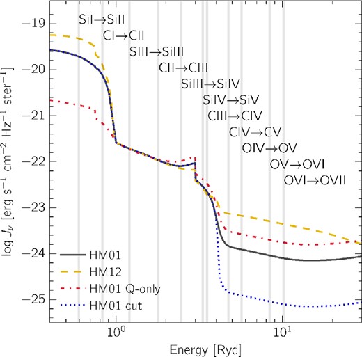
Comparison of different extragalactic ionization backgrounds.
As a first test, we examine the values of [O/H] derived when we assume PIE with T = 2 × 10⁴ K for the four different backgrounds in Fig. C2. We find that for the first three backgrounds (HM01, HM12, and Q-only) the results are in fairly good agreement. In general, the metallicity–density relation is steepest for HM01, and spans the largest range of [O/H] values.
![[O/H] derived from the O vi(H i) relation, for four different extragalactic backgrounds (as indicated in each panel), under the assumption of PIE.](https://oup.silverchair-cdn.com/oup/backfile/Content_public/Journal/mnras/450/2/10.1093/mnras/stv750/2/m_stv750figc2.jpeg?Expires=1750525765&Signature=faUKcAbrVZs-amsMUOD0wemQhwbVlUPjxncU5RGuV0r8QGYxBlzMXpSTftueObrlB9NRXLVQdHrDy~JDbbEvQ~ARtDv7g6FpRQprUZYDiY-DA8HWZHnUP6tEqbyzEsSwwAS2378bkluZa68GLd-Vm2sBke4wNXgdvp~q9fxHl9kP~qbZdckVHRwElVgU7UXm8DZ4suz5ZE3N59hjT41EWK50yhUP-6-d2IcKR7V6lDpupBnEd6DM~oRuS4HOIUawqhaH5th-~vfB5Jf99mAay6xnWk~WXqcwYIE1KPH6t~4ea~-6EfE7PP7W~Z1mrZKOpE3Szqi02UVNTG2jtDNXvQ__&Key-Pair-Id=APKAIE5G5CRDK6RD3PGA)
[O/H] derived from the O vi(H i) relation, for four different extragalactic backgrounds (as indicated in each panel), under the assumption of PIE.
Of the four backgrounds considered, the one salient outlier is the HM01 cut background (bottom right-hand panel). First, for the small galactocentric distance points, invoking this background produces reasonable (i.e. at least less than solar) metallicities for |$\log _{10} \tau _{\rm H\, {\small I}} < 1$|. However, the qualitative behaviour of inferred [O/H] as density decreases is still present. Furthermore, for |$\log _{10} \tau _{\rm H\, {\small I}} > 1$|, the inferred metallicities of the full pixel sample become unrealistically high (up to [O/H] ∼1, while Steidel et al. 2014 find Z = 0.4 Z⊙ for this galaxy sample), suggesting that this background is not a realistic choice.
Another significant change that would result from using the HM01 cut model is shown in Fig. C3, where we compare the values of |$\log _{10}\tau _{\rm O\,\small {vi}}/\tau _{\rm C\,\small {iv}}$| as a function of temperature and density for both the HM01 (solid black contours) and HM01 cut (dashed blue contours) backgrounds.
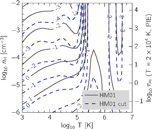
The predicted values of |$\log _{10} \tau _{\rm O\,\small {vi}} / \tau _{\rm C\,\small {iv}}$| for the HM01 (black solid contours) and HM01 cut (blue dashed contours) backgrounds.
The observed ratios span values that range from ∼100 to 101 for the small galactocentric distance sample. For the HM01 background, this corresponds to gas that has either log10nH ∼ −5 to −4 cm−3 at T ∼ 2 × 10⁴ K, or log10nH ≳ −4.5 cm−3 at T ∼ 105.4 K. However, for HM01 cut, at the typical photoionized gas temperature of T ∼ 2 × 10⁴ K, log10nH ≲ −5.2 cm−3 for the range of observed optical depths, which corresponds to underdense values (i.e. Δ < 1). Although the small galactocentric distance pixel sample could be reconciled with temperatures of T ∼ 105.4 K, it is unlikely that the full pixel sample is typically probing such hot gas, or densities below the cosmic mean. We conclude that the HM01 cut background is in tension with ratios of |$\tau _{\rm O\,\small {vi}}/\tau _{\rm C\,\small {iv}}$| derived from the full pixel sample.
