


Abstract
We investigate the properties of haloes, galaxies and black holes to z = 0 in the high-resolution hydrodynamical simulation MassiveBlack-II (MBII) which evolves a Λ cold dark matter cosmology in a comoving volume Vbox = (100 Mpc h−1)3. MBII is the highest resolution simulation of this size which includes a self-consistent model for star formation, black hole accretion and associated feedback. We provide a simulation browser web application which enables interactive search and tagging of the MBII data set and publicly release our galaxy catalogues. We find that baryons affect strongly the halo mass function (MF), with 20–33 per cent change in the halo abundance below the knee of the MF (Mhalo < 1013.2 M⊙ h−1 at z = 0) when compared to dark-matter-only simulations. We provide a fitting function for the halo MF out to redshift z = 11 and discuss its limitations. We study the halo occupation distribution and clustering of galaxies, in particular the evolution and scale dependence of stochasticity and bias finding reasonable agreement with observational data. The shape of the cosmic spectral energy distribution of galaxies in MBII is consistent with observations, but lower in amplitude. The Galaxy stellar mass function (GSMF) function is broadly consistent with observations at z ≥ 2. At z < 2, the population of passive low-mass (M* < 109 M⊙) galaxies in MBII makes the GSMF too steep compared to observations whereas at the high-mass end (M* > 1011 M⊙) galaxies hosting bright AGNs make significant contributions to the GSMF. The quasar bolometric luminosity function is also largely consistent with observations. We note however that more efficient AGN feedback is necessary for the largest, rarest objects/clusters at low redshifts.
1 INTRODUCTION
The cold dark matter model with a cosmological constant (ΛCDM) is well established enough (see e.g. Hinshaw et al. 2013; Crandall & Ratra 2014; Lahav & Liddle 2014; Planck Collaboration XVI 2014) that individual large-scale simulation efforts can be carried out that focus on just this one cosmology. We have also reached the point at which supercomputers enable numerical modelling of cosmological volumes with enough resolution to study the properties of individual galaxies. In this paper, we report on a P-GADGET hydrodynamic simulation of 100 h−1 Mpc cubic volume, the MassiveBlack-II (MBII) simulation. It has ∼106 M⊙ mass resolution, cooling, star formation, black holes (BHs) and feedback, and represents the evolution of a ΛCDM universe to redshift z = 0.
Numerical simulations (see reviews by Bertschinger 1998; Dolag et al. 2008; Springel 2012) are the tool of choice to address many questions in cosmology, as galaxy formation is a complex non-linear problem. Two criteria which must be satisfied for accurate results are as follows.
A large enough simulation volume that Fourier density modes on the largest scales are evolving independently. The volume simulated must be a representative region of the Universe, otherwise inferences drawn from it regarding such questions as clustering and the mass function (MF) of objects will be incorrect (Bagla & Ray 2005; Bagla & Prasad 2006; Orban 2013). When ΛCDM models are evolved to redshift z = 0, then a volume of at least ∼100 h−1 Mpc on a side becomes necessary to predict the overall star formation rate (SFR), for example Springel & Hernquist (2003b).
High enough mass and spatial resolution that the properties of the objects of interest have converged. This requires many resolution elements (particles or grid cells). If we focus on particle based simulations relevant to the current work, at the very least for identification of objects there must be enough particles to overcome shot noise. If we require detailed properties of the objects such as galaxy spectra, or angular momenta then this can require many more(e.g. Governato et al. 2007).
These criteria of large simulation volume and high resolution are more straightforward to address in the context of more restricted physical modelling. As a result, dark matter- and gravity-only simulations have long been used to make cosmological predictions that cover both large and small scales in the same volume (e.g. Springel et al. 2005b; Boylan-Kolchin et al. 2009; Klypin, Trujillo-Gomez & Primack 2011). Semi-analytic modelling has been used to process dark matter simulations, resulting in many studies of the galaxies and their properties in the ΛCDM model (see e.g. Baugh 2006; Hirschmann et al. 2012 and references therein).
Baryonic physics including hydrodynamics obviously plays an important role in the formation of luminous objects and structure. This has led to the inclusion of the relevant equations in simulation codes in many forms, smoothed particle hydrodynamics (SPH; Monaghan 1992), Eulerian grid solvers (e.g. Cen 1992; Bryan & Norman 1997) and hybrid Lagrangian/Eulerian schemes (e.g. Springel 2010). Although previous work has not simultaneously reached the combination of large volume and high resolution that we present here, research has progressed using many methods, including making use of zoom simulations of smaller volumes inside a representative one (Katz & White 1993; Scannapieco et al. 2012), simulations that stop at high redshifts before large-scale modes become non-linear (e.g. Di Matteo et al. 2012), or by tackling problems which require lower mass resolution (e.g. Battaglia et al. 2012).
The advent of large-scale computing facilities with 100 000 compute cores or more (such as the Cray XT5, ‘Kraken’ on which the current simulation was run) and the development of highly efficient distributed memory simulation codes (such as GADGET2; Springel 2005) means that simulations which satisfy both criteria (1) and (2) are now possible. We have run one such simulation as part of the NSF Petascale applications in cosmology programme, using the code P-GADGET (see e.g. Di Matteo et al. 2012).
Our aim was to simulate and analyse a large, representative volume of the ΛCDM model with the most important physical processes previously included in zoom runs or simulations with smaller boxes. These are hydrodynamics (using SPH), cooling, a subgrid multiphase model for star formation (Springel & Hernquist 2003a) and subgrid BH modelling (Di Matteo, Springel & Hernquist 2005; Springel, Di Matteo & Hernquist 2005a), both with feedback. Our use of the physical modelling and algorithms used in previous work such as Di Matteo et al. (2008), Croft et al. (2009), Degraf, Di Matteo & Springel (2010) and Di Matteo et al. (2012) enables continuity and therefore comparison with this previous work. Our aim is to see what this ‘fiducial’ model (ΛCDM + GADGET SPH + the particular subgrid algorithms employed) predicts about the properties of galaxies, their haloes and their clustering at redshifts extending down to the present day. We have not adjusted methods, algorithms and parameters used in previous work (e.g. DeGraf et al. 2012) to try to tune to observational results. Our goal is to see how this model performs, now that there is a large volume at high resolution. We naturally expect both regions of agreement and disagreement with observations and we aim that our work will offer guidance to future work to address the problems.
In this paper, we make the first use of the MBII simulation evolved to z = 0, and use it to explore some topics in structure formation. Here, we choose to focus on topics relevant to galaxy and AGN formation and large-scale structure, including MFs, galaxy and halo properties and clustering. Our emphasis is on lower redshifts; the simulation at redshifts z > 5 has been explored by Wilkins et al. (2013a,b,c). Topics that we leave to future work include the intergalactic medium (IGM), absorption lines, galaxy clusters and X-ray emission.
Our plan for the paper is as follows. In Section 2, we briefly describe the numerical methods and algorithms used to run the simulation, select galaxies and carry out stellar population synthesis (SPS). In Section 3, we describe visualization of the simulation. In Sections 4.2 and 5, respectively, we present the MF and halo occupation distribution (HOD) and in Section 6 we examine the clustering of dark matter and galaxies. The properties of galaxies and supermassive BHs are examined in Sections 7 and 8 and we derive some conclusions from our work in Section 9. We make comparison with observations whenever it is directly possible to do so. In many cases, observational bias needs to be taken into account and a direct comparison is not always possible. In addition to observational bias the errors associated with them are based on estimated systematics, finite sample, detector noise and instrument resolution to name a few. The interested reader is encouraged to refer to the observational work cited here for further clarification of observational data and associated errors.
2 METHODS
2.1 Numerical code
We have used P-GADGET, an upgraded version of GADGET3 (see Springel 2005 for an earlier version) which we are developing for use at upcoming Petascale supercomputer facilities. This code was also used to run the MassiveBlack (MB) simulation (Di Matteo et al. 2012). Both MB and MBII are cosmological simulation of a ΛCDM cosmology. The major differences between MB and MBII are resolution and volume. However there are minor differences in cosmology between the two. The other difference between MB and MBII is final redshift zf to which the simulation proceeded. MB was run to zf = 4.75 and was used to study the high-redshift Universe whereas MBII proceeded all the way to z ∼ 0. Additionally, we have run a dark-matter-only (DMO) variant of MBII which we refer as MBII-DMO (with the same initial conditions, particle number and volume as MBII) to compare the effects of baryons on the MF and the correlation function of dark matter. Details of MB, MBII and MBII-DMO are listed in Table 1.
Basic simulation parameters for the simulation. The columns list the simulation, the size of the simulation box, Lbox, the number of particles (dark matter + gas) used in the simulation, Npart, the mass of a single dark matter particle, |$m_{_{\mathrm{DM}}}$|, the initial mass of a gas particle, |$m_{_{\mathrm{gas}}}$|, and the gravitational softening length, ϵ. The last column is the redshift zf to which the simulation proceeded. All length-scales are in comoving units. The rows are for the MB, MBII and MBII-DMO simulations.
| Simulation | Lbox | Npart | |$m_{_{\mathrm{DM}}}$| | |$m_{_{\mathrm{gas}}}$| | ϵ | zf |
|---|---|---|---|---|---|---|
| (h−1 Mpc) | (h−1 M⊙) | (h−1 M⊙) | (h−1 kpc) | |||
| MB | 533.333 | 2 × 32003 | 2.78 × 10⁸ | 5.65 × 10⁷ | 5 | 4.75 |
| MBII | 100 | 2 × 17923 | 1.1 × 10⁷ | 2.2 × 10⁶ | 1.85 | 0.0625 |
| MBII-DMO | 100 | 2 × 17923 | 1.32 × 10⁷ | – | 1.85 | 0 |
The initial conditions for MBII were generated with the cmbfast transfer function at z = 159 and the simulation was evolved to z = 0. The cosmological parameters used were: amplitude of mass fluctuations, σ8 = 0.816, spectral index, ns = 0.968, cosmological constant parameter ΩΛ = 0.725, mass density parameter Ωm = 0.275, baryon density parameter Ωb = 0.046 and h = 0.701 (Hubble's constant in units of 100 km s−1 Mpc−1). These are consistent with the Wilkinson Microwave Anisotropy Probe 7 cosmology (Komatsu et al. 2011). The initial conditions and realization of MBII-DMO are identical to MBII.
2.2 Halo and subhalo identification
We identify haloes with the friends-of-friends (FOF) procedure (Davis et al. 1985) applied to dark matter particles with a linking length of b = 0.2 times the mean interparticle separation. Gas, stars and BHs are then associated to their nearest dark matter particles. The subhalo finder subfind (Springel et al. 2001) was then used, working with particles in the FOF halo and computing a local density for each particle. Starting from isolated density peaks within the FOF halo, additional particles with decreasing density are attached to it. Whenever a saddle point, which connects two disjoint overdensities is reached, the smaller of the two is treated as a substructure candidate followed by merging of the two regions. Eventually all particles within a substructure are checked for self-boundedness and only those particles are retained which have a total negative energy. We define galaxies to be the haloes identified with SUBFIND with at least 64 star particles.
2.3 Subgrid model for star formation BH growth and associated feedback
The subgrid models for star formation, BH growth and associated feedback processes are identical to that employed in the MB simulation. We briefly describe them here and refer the reader to the MB simulation (e.g. Di Matteo et al. 2012) for a more detailed description.
We adopt the multiphase model for star-forming gas developed by Springel & Hernquist (2003a). This has two principal ingredients: (1) a star formation prescription and (2) an effective equation of state (EOS). (1) is motivated by observations and given by the Schmidt–Kennicutt Law (Kennicutt 1989), where the SFR is proportional to the density of cold clouds (|$\rho _{\rm SFR} \propto \rho _{{\rm gas}}^{N}$| and N = 1.5. Star particles are created from gas particles probabilistically according to their SFRs. (2) encapsulates the self-regulated nature of star formation due to supernovae feedback in a simple model for a multiphase interstellar medium (ISM). In this model, a thermal instability is assumed to operate above a critical density threshold ρth, producing a two phase medium consisting of cold clouds embedded in a tenuous gas at pressure equilibrium. Stars form from the cold clouds, and short-lived stars supply an energy of 1051 erg to the surrounding gas as supernovae. This energy heats the diffuse phase of the ISM and evaporates cold clouds, thereby establishing a self-regulation cycle for star formation. ρth is determined self-consistently in the model by requiring that the EOS is continuous at the onset of star formation. The cloud evaporation process and the cooling function of the gas then determine the temperatures and the mass fractions of the two ‘hot and cold’ phases of the ISM, such that the EOS of the model can be directly computed as a function of density. In addition, a parametrization of stellar winds is also used (see Springel & Hernquist 2003a, for further details).
In MBII, BHs are modelled as collisionless sink particles within newly collapsing haloes, which are identified by the FOF halofinder called on the fly at regular time intervals. A seed BH of mass Mseed = 5 × 10⁵ h−1 M⊙ is inserted into a halo with mass Mhalo ≥ 5 × 10¹⁰ h−1 M⊙ if it does not already contain a BH. Once seeded, BHs grow by accreting gas in its surrounding region or by merging with other BHs. Gas is accreted with an accretion rate |$\dot{M}_{\mathrm{BH}} = \frac{4\pi G^2 M_{_{\mathrm{BH}}}^2 \rho }{\left(c_{\rm s}^2 + v_{\mathrm{BH}}^2\right)^{3/2}}$|, where vBH is the velocity of the BH relative to the surrounding gas, ρ and cs are the density and sound speed of the hot and cold phase of the ISM gas (which when taken into account appropriately as in Pelupessy, Di Matteo & Ciardi 2007 eliminates the need for a correction factor α previously introduced). We allow the accretion rate to be mildly super-Eddington but limit it to a maximum allowed value equal to 2 × Eddington rate (|$\dot{M}_{\mathrm{Edd}}$|) to prevent artificially high values, consistent with Begelman, Volonteri & Rees (2006) and Volonteri & Rees (2006). The BH radiates with a bolometric luminosity which is proportional to the accretion rate, |$L_{\mathrm{bol}}= \eta \dot{M}_{\mathrm{BH}}c^2$| (Shakura & Sunyaev 1973), where η is the radiative efficiency and its standard value of 0.1 is kept throughout, and c is the speed of light. In the simulation, 5 per cent of the radiated energy couples thermally to the surrounding gas and this energy is deposited isotropically on gas particles that are within the BH kernel (64 nearest neighbours) and acts as a form of feedback (Di Matteo et al. 2005). The value of the feedback energy parameter, f = 0.05, is kept constant and is the only free parameter in the model and was set using galaxy merger simulations (Di Matteo et al. 2005) to match the normalization in the observed |$M_{_{\mathrm{BH}}}{\rm -}\sigma$| relation. BHs also grow by merging once one BH comes within the kernel of another with a relative velocity below the local gas sound speed.
This model for the growth of BHs has been developed by Di Matteo et al. (2005) and Springel et al. (2005a). It has been implemented and studied extensively in cosmological simulations (Li et al. 2007; Sijacki et al. 2007; Colberg & Di Matteo 2008; Di Matteo et al. 2008; Booth & Schaye 2009; Croft et al. 2009; Sijacki, Springel & Haehnelt 2009; Degraf et al. 2010, 2011b; Degraf, Di Matteo & Springel 2011a; Chatterjee et al. 2012), successfully reproducing basic properties of BH growth, the observed |$M_{_{\mathrm{BH}}}{\rm -}\sigma$| relation and the BH MF (Di Matteo et al. 2008), the quasar luminosity function (QLF; Degraf et al. 2010) at z ≥ 0.5 and the clustering of quasars (Degraf et al. 2011a).
2.4 Stellar population synthesis
The spectral energy distribution (SED) of a galaxy is generated by summing the SEDs of each star particle in the galaxy. The SED of the star particles is generated using the pegase.2 SPS code (Fioc & Rocca-Volmerange 1997, 1999) by considering their ages, mass and metallicities and assuming a Salpeter initial mass function (IMF). Nebula (continuum and line) emission is also added to each star particle SED. We also apply a correction for absorption in the IGM using the standard Madau et al. (1996) prescription. We finally sum the SED of each galaxy and convolve with given filters (see bottom panels of Fig. 17) to finally obtain the broad-band photometry, hence the CSED.
2.5 Public release of MBII galaxy catalogues
We release the MBII galaxy catalogues to the scientific community. Some of the properties included in these catalogues are position, velocity, mass, mass by particle type (such as gas, dark matter, stars and BHs), circular velocity and rest-frame luminosities. We encourage the community to use these galaxy catalogues which can be accessed from http://mbii.phys.cmu.edu/data/. A more detailed description and sample codes can also be found at the above URL.
3 VISUALIZATION
To enable easy visual exploration of the large data set represented by the MassiveBlack 2 simulation, we have developed an interactive simulation browser web application. The browser allows real-time zooming, panning in the simulation, and enables searching and locating of haloes and subhaloes in the simulation. The application is built upon existing web technology. Two main libraries used are Gigapan,1 and the Microsoft Seadragon library.2
Fig. 1 shows the interface for the interactive browser. The browser can be accessed from the URL http://mbii.phys.cmu.edu. It consists of a viewport and three floating control panels: the MAIN panel, located at the top-right corner of the interface; the INFOrmation panel, located at the left-hand side of the interface; and the NAVigation panel, located at the bottom-right corner of the interface.

Interface for the interactive simulation browser.
The Gigapan image of the selected snapshot is displayed in the viewport, where subhaloes are also marked with green crosses. In addition, central subhaloes (Msubhalo > 0.1Mgroup) are labelled with an additional circle. Interactive zooming and panning in the viewport is implemented via mouse clicking and dragging.
The MAIN panel provides the following functionalities:
selecting an epoch from the snapshot number;
switching between the gas and stellar image layer;
jumping among FOF groups;
querying subhaloes in the current view.
The INFO panel displays the properties of the currently selected subhalo or group. In Fig. 1, for example, the panels shows the property of the currently selected subhalo (marked with a rectangle).
The NAV panel provides zoom-in and zoom-out controls, and a switch to toggle the visibility of other control panels.
Fig. 2 shows a collage of images extracted from the browser. In this example, we have selected three haloes in the simulation at redshift z = 1.0: (I) at a major confluence of filaments; (II) a moderately sized halo with three main subhaloes; (III) a relatively isolated halo. For each of the halo we show the stellar component in their subhaloes, embedded in their surrounding gas environment.

Visualization of MBII simulation. The central panel, O shows the full simulation box: the z = 1.0 snapshot is mapped into an 8 h−1 Mpc thick slice. Panels I, II and III show the gaseous environment of three FOF groups. Panel (a)–(f) show the stellar component of the subhaloes. The central subhaloes are marked with dots, and 10 of the brightest subhaloes are marked with stars. Please see the text for a description of the colour scheme. The interactive simulation browser is available at http://mbii.phys.cmu.edu.
The gigapan images used in the browser are high-resolution 2D images of the full simulation rendered with the visualization software gaepsi (Feng et al. 2011). The gas images (panels O, I, II, III) are rendered with the divergent cool–warm colour-map introduced by Moreland (2009). The density information is encoded in the brightness of the pixels; brighter pixels have higher column density, and voids are represented with black (zero-brightness). The temperature of gas is encoded in the hue of the pixels, blue represents low temperature (T < 103.5 K), and red represents high temperature (T > 107.5 K). The stellar images (panels a, b, c, d, e and f) are composed from the simulated i-, r- and g-band luminosity. This band definition follows the convention used by the Sloan Digital Sky Survey (SDSS; see the procedure described in Lupton et al. 2004).
4 MF OF HALOES
Given that dark matter haloes represent the locations where gas can cool and form stars and galaxies, it is important to predict their abundances – the halo MF – accurately. The halo or subhalo MF, is one of the fundamental quantities in structure formation. It is an important ingredient in a diverse set of tools used for making theoretical predictions in cosmology. At low redshifts, the tail of the MF which probes the abundance of clusters is extremely sensitive to cosmological parameters. It is also a key component in studying the clustering of galaxies as the halo–halo term (see Cooray & Sheth 2002) depends on the MF. At higher redshifts, the MF is used in modelling the sources of reionization which reside in dark matter haloes like PopIII stars, early galaxies and quasars. Any significant deviation in the MF as predicted by the ΛCDM model would therefore create some tension in our current understanding of structure formation. It is therefore very important to quantify systematic effects arising from baryonic processes on the distribution of matter since they will lead to a systematic error on the inferred cosmological parameters (Wu, Zentner & Wechsler 2010). This has been studied for example in the context of the matter power spectrum and the cumulative MF at z = 0 (Rudd, Zentner & Kravtsov 2008) and the abundance of massive haloes (Stanek, Rudd & Evrard 2009; Cui, Borgani & Murante 2014). However, these simulations covered a limited dynamic range in halo mass and/or employed much simpler subgrid models for baryonic processes.
Traditionally dark matter simulations have been used to compute the abundance of haloes for a given cosmology. A key component of these analyses is the halo definition. The FOF definition identifies regions bounded by an isodensity contour whereas the spherical overdensity (SO) definition identifies an artificial spherical region centred on a density maximum such that the density within it is at a given density threshold. A dark matter halo is never perfectly spherical making the SO definition artificial. The FOF definition is prone to artificially bridging two (or more) nearby haloes connected by a filament.
In this section, we will not look at how the halo definition affects the MF predicted by MBII since much work has been done on this subject (Lacey & Cole 1994; Jenkins et al. 2001; White 2002; Tinker et al. 2008; Watson et al. 2013). We will rather choose a halo definition and see how baryonic effects affect the MF and compare our results with fitting functions based on DMO simulations and the MBII-DMO simulation.
We generate two catalogues of haloes based on the FOF and SUBFIND halofinders. For the SUBFIND cataloguer, we do not distinguish between centrals and satellites in this section. These catalogues contain the total number of particles by type (e.g. gas, dark matter, stars and BHs), and the total mass by type amongst other important halo properties. For the analysis in this section, we consider the smallest halo to have a resolution limit of 40 particles by type. E.g. An object is considered to be a halo if its mass satisfies Mhalo ≥ 40 × (mdm + mgas), where mdm and mgas are given in Table 1. If we are interested only in the dark matter component of the halo then the above condition is relaxed such that Mhalo ≥ 40 × mdm. Note that these criteria affect the statistics and counts of only the smallest haloes.
In the case of dark matter simulations, it has been shown (Warren et al. 2006) that haloes with small particle counts have a mass which is systematically overestimated. Corrections have been proposed to alleviate this (Warren et al. 2006; Lukić et al. 2009; Bhattacharya et al. 2011; More et al. 2011). We choose to ignore for this effect for three reasons. (1) It is not clear how such corrections apply to each particle type in MBII. Providing a similar correction to halo masses for hydrodynamical simulations is beyond the scope of this paper. (2) In Section 4.2, we will show that the baryonic effects already show up in the halo MF at lower masses at the 10–33 per cent level when compared to dark matter simulations. A correction to the mass of the halo at smaller masses will only enhance the discrepancy in the MF. (3) Given our halo definition, we can directly compare MBII and MBII-DMO; any correction should affect both in a similar manner.
The largest mode that any cosmological simulation can sample is governed by the physical size of the simulation volume. Large-scale modes k < 2π/Lbox are not sampled in the simulation and lead to a suppression of structure formation and hence the MF. This is a well-known effect (Bagla & Ray 2005; Sirko 2005; Bagla & Prasad 2006) and masses can be corrected by accounting for the missing power (Reed et al. 2007; Watson et al. 2013). Bagla & Ray (2005) point out that a boxsize Lbox = 100 h−1 Mpc is sufficient to obtain reasonably reliable MFs to halo masses Mhalo ≲ 1014 M⊙ h−1 for the ΛCDM model at z = 0; the requirement for large boxes becomes less stringent at higher redshift. Our focus will in any case be for smaller masses, which are less affected by effects of finite volume. We therefore choose not to make any corrections to the MF due to missing large-scale power. Secondly, since we are directly comparing MBII and MBII-DMO, which are equally affected by finite volume, such a correction is not required.
4.1 The baryon fraction of haloes
We start by looking at the baryon fraction of haloes in Fig. 3 as a function of halo mass. We plot the ratio of the baryon fraction of haloes to the cosmic baryon fraction |$f_{\rm b}^{{\rm halo}}/f_{\rm b}^{\rm cosmic}$| where |$f_{\rm b}^{{\rm cosmic}} = \Omega _{\rm b}/\Omega _{\rm m}$| and |$f_{\rm b}^{{\rm halo}}$| is the ratio of baryonic to total mass of the halo. The solid line represents haloes identified with the FOF algorithm whereas the dot–dashed line represents those identified by SUBFIND.
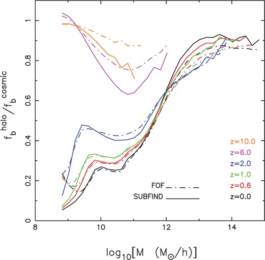
The evolution of the baryon fraction of haloes (|$f_{\rm b}^{{\rm halo}}$|) in units of the cosmic baryon fraction |$f_{\rm b}^{{\rm cosmic}}$| as a function of halo mass. The solid line is for FOF haloes and the dot–dashed is for haloes identified with SUBFIND. The colours (black, red, green, blue, pink and orange) represent the baryon fraction for different redshifts (z = 0.0, 0.6, 1, 2, 6, 10).
We find that the distinction between haloes and subhaloes has little effect on the baryon fraction of haloes below z = 6. At z ≥ 6, the baryon fraction of subhaloes identified with SUBFIND is larger compared to objects identified with FOF although the qualitative trend with mass is similar. We find that the baryon fraction plateaus to around 80–90 per cent around Mhalo ≥ 1013 M⊙ h−1 at low redshifts and drops significantly below that mass scale. A direct comparison with observed baryon fractions for clusters (Andreon 2010) is difficult at this point given that these observations relate stellar and gas fractions at different scales, e.g. r200 for stellar fractions and r500 for gas fractions. At this point, it is worthwhile to compare our results with Crain et al. (2007) who looked at the baryon fraction of haloes in an adiabatic resimulation of the Millennium simulation and another smaller volume (higher resolution) simulation at z = 0. These authors also included an additional simulation with a simple photoheating model, where a gas temperature floor of Tfloor = 2 × 10⁴ K was assumed to mimic the IGM temperature at mean density in the post-reionized Universe. Star and BH formation and associated feedback processes were not included. These authors found that the baryon fraction plateaued to around 90 per cent for Mhalo ≥ 1010 M⊙ h−1 and dropped significantly below that in their photoionization model, whereas the baryon fraction in the adiabatic simulation did not show any significant behaviour with halo mass. Our results largely agree well the results of Crain et al. (2007), for larger masses however, we find that feedback can drastically prevent the collapse of baryons in haloes below Mhalo ≲ 1013 M⊙ h−1. Crain et al. (2007) found that photoionization regulates the formation of smaller galaxies with Mhalo ≲ 1010 M⊙ h−1. Interestingly, we find that at Mhalo ∼ 1010 M⊙ h−1 the baryon fraction plateaus to around 20–40 per cent of the cosmic mean. It drops below that mass scale, which can be attributed to photoheating. The suppression of the baryonic fraction in Mhalo = 1010–1013 M⊙ h−1 can be attributed to feedback from stars and BHs.
Since we see that baryon effects play an important role in the formation of haloes, we expect to see deviations in the halo MF which is the premise of the next section.
4.2 The mass function
We use the FOF and SUBFIND algorithms to compute the halo and subhalo MFs, respectively. We look at the total halo/subhalo mass and the mass of the dark matter component. In Section 7, we will look at the galaxy stellar mass function (GSMF) and compare them with observational constraints. In this analysis, we choose the mass bin to be Δlog M = 0.2 which is well within the recommended bin width (Lukić et al. 2007) to avoid any systematic error that may arise in the estimate of the MF due to large bins. We assume Poisson errors for the counts of haloes in this mass bin.
In Fig. 4, we plot the rescaled MF f(σ) for redshifts z = 10–0 from the MBII simulation (open squares, blue to red). For the FOF MFs, we also add data from the MB simulation from redshifts z = 11 to 5 (open circles purple to green). Each panel is split into two: in the top part of the panel we plot ln [f(σ)] versus ln [σ−1] where as in the bottom part of the panel we compare it with the Sheth & Tormen (2002) MF and plot their difference. To guide the eye, we have added a reference (dot–dashed y = 0)horizontal line. For any simulation, the MF data points move from right to left along a single curve in the f(σ)–σ plane with decreasing redshift. The top row and bottom rows denote the SUBFIND and FOF MFs. The columns denote the full mass of the halo and the dark matter mass of the halo, respectively. The dashed (red), dot–dashed (cyan), triple-dot–dashed (orange) lines are for the MFs from Press & Schechter (1974), Sheth & Tormen (2002) and Watson et al. (2013) The solid (black) line in the bottom panels (FOF MFs) denote the best-fitting MF to the MB and MBII data based on the Tinker et al. (2008) parametrization of the Warren et al. (2006) MF.
![The SUBFIND (top) and FOF (bottom) MFs are plotted from z = 0–11. Each panel is split into two; in the top part of the panel we plot ln [f(σ)] versus ln [σ−1] where as in the bottom part of the panel we plot the difference between ln [f(σ)] and the Sheth & Tormen (2002) MF. To guide the eye, we have added a reference (dot–dashed y = 0)horizontal line. The columns denote the MF based on the total halo mass and the dark matter component of the halo mass, respectively. The open squares denote data points from the MBII simulation from z = 0–10 (red-blue). The open circles in the FOF MF (bottom panels) denote data from the MB simulation from z = 5–11 (green-purple). The dashed (red), dot–dashed (cyan), triple-dot–dashed (orange) lines are for the MFs from Press & Schechter (1974), Sheth & Tormen (2002) and Watson et al. (2013). The solid (black) line in the bottom panels (FOF MFs) denote the best-fitting MF to the MB and MBII data based on the Tinker et al. (2008) parametrization of the Warren et al. (2006) MF.](https://oup.silverchair-cdn.com/oup/backfile/Content_public/Journal/mnras/450/2/10.1093/mnras/stv627/2/m_stv627fig4.jpeg?Expires=1750240227&Signature=GKO6zJbakwqJ71cT9aZJ9jOL9Q6wI3pGddsCSHOXKrZkI8IH8D5jpGg7Yv1M8JiqS6QwqaPmWYJbd1g5oh1R7Cq2QzRxnEq6K0zVxjxDAtYuZwH40PccTj-mAPBTu7UEIMiya7htqMCYD6IrdGLtQ2j7bFJKQN9IQWmm-bjOVabcGtXRXSh6lIdWvLjO0fhzGXzQJa6O94wVV2hogWX1E7FAWh2rSDvlgaB1aQmRuE8pCk9nQRRXaPugOUg6zh4Sv-wJgcNnSAFk8EcreE1J33zcjCQkZ9jYu-KsaNMgxgewYtEskooF8JgO6d718xlLzuXo19sZ4NsB4nR8jXp-HQ__&Key-Pair-Id=APKAIE5G5CRDK6RD3PGA)
The SUBFIND (top) and FOF (bottom) MFs are plotted from z = 0–11. Each panel is split into two; in the top part of the panel we plot ln [f(σ)] versus ln [σ−1] where as in the bottom part of the panel we plot the difference between ln [f(σ)] and the Sheth & Tormen (2002) MF. To guide the eye, we have added a reference (dot–dashed y = 0)horizontal line. The columns denote the MF based on the total halo mass and the dark matter component of the halo mass, respectively. The open squares denote data points from the MBII simulation from z = 0–10 (red-blue). The open circles in the FOF MF (bottom panels) denote data from the MB simulation from z = 5–11 (green-purple). The dashed (red), dot–dashed (cyan), triple-dot–dashed (orange) lines are for the MFs from Press & Schechter (1974), Sheth & Tormen (2002) and Watson et al. (2013). The solid (black) line in the bottom panels (FOF MFs) denote the best-fitting MF to the MB and MBII data based on the Tinker et al. (2008) parametrization of the Warren et al. (2006) MF.
The PS MF (Press & Schechter 1974) overpredicts the abundance of low-mass haloes and underpredicts the abundance of large mass haloes. This has been seen in numerous studies (Sheth & Tormen 1999; Jenkins et al. 2001; Lukić et al. 2007; Reed et al. 2007; Watson et al. 2013). This has led to a renewed effort in recent years to recalibrate the MF of haloes based on simulations.
We find that the SUBFIND MFs for haloes and dark matter do not fall on a single curve. There is significant and systematic scatter across redshifts at small masses. The deviations from a redshift independent function typically occur at intermediate-lower masses for each redshift and is particularly visible around the knee of the MF. This can be clearly seen in the difference plot where we see an upturn at lower masses. This is similar to the analyses of Jenkins et al. (2001), Tinker et al. (2008) and Watson et al. (2013) who found that the MF deviated from a universal form more strongly (having a redshift dependence), when they considered a halo definition different from FOF. We therefore do not provide a universal fit to the SUBFIND MFs which show a strong redshift dependence.
On the other hand, the FOF MF has been shown to be more universal (Jenkins et al. 2001; Bhattacharya et al. 2011; Watson et al. 2013) and this is also seen in the lower panels of Fig. 4. We denote FOF and FOFD to represent the FOF halo and dark matter component of the FOF halo. We find that the FOF and FOFD MFs agree well with the Sheth & Tormen (2002) and Watson et al. (2013) MFs at the larger masses. The FOFD shows a systematic shift with respect to the FOF MF due to a systematic shift in the halo mass, since the baryon contribution has been subtracted from the halo mass. However, the MF at small masses is systematically underestimated in MBII. This discrepancy is larger for FOFD which is again due to a systematic shift in the halo mass. Our results are consistent with Sawala et al. (2013) who used the set of simulations described in Crain et al. (2009) to look at the effect of baryons on the abundance of haloes. Sawala et al. (2013) compared the Galaxies-Intergalactic Medium Interaction Calculation (GIMIC) (which include gas, dark matter, star formation and feedback) and the DMO simulations (Crain et al. 2009) which were performed by resimulating at higher resolution an 18 h−1 Mpc spherical region of the Millennium simulation (Springel et al. 2005b). Both the GIMIC and DMO runs were done with the same initial conditions making it possible to look at the effect of baryons on halo properties directly. They found that both simulations agree well on large scales however objects below ∼1012 M⊙ have systematically lower masses in the GIMIC simulation when compared to the DMO counterpart. This result translated to an overestimate of the abundance of structures in the DMO simulation, by approximately ∼10 per cent at 1011.5 M⊙ and ∼30 per cent at 1010 M⊙. We compare the MBII MF with published dark matter simulations and MBII-DMO next.

Left: comparison of the FOF MF in MBII (open red squares) is made with the MBII-DMO simulation (blue crossed circles) in a redshift independent manner. Similar to Fig. 4 in the bottom part of the panel we make a comparison with the Sheth & Tormen (2002) MF by plotting their difference. The solid (black) line is the fit based on MB and MBII data. The dotted line is the fit based on the MBII-DMO data from z = 10 to z = 0. Right: ratio of the best-fitting FOF MF with fits based on DMO simulations and MBII-DMO for FOF haloes. The solid (black) horizontal line is for the combined data of MB and MBII. The solid (red), dashed (cyan), dot–dashed (blue), dotted (green) and triple-dot–dashed (orange) lines are from Jenkins et al. (2001), Sheth & Tormen (2002), Warren et al. (2006), Bhattacharya et al. (2011) and Watson et al. (2013). The dot–dashed (black) line is for the MBII-DMO fit. The grey shaded box highlights the region below the knee of the MF where dark matter simulations systematically overpredict the abundance of haloes.
Best-fitting parameters for the FOF and FOFD MFs using the combined MB and MBII data (first two rows). The third row is the best-fitting parameters for the FOF MF using MBII-DMO data only. The parameters are described in equation (5). The last row is the best-fitting parameters from Watson et al. (2013).
| A | α | β | γ | |
|---|---|---|---|---|
| FOF (MB+MBII) | 0.1897 | 1.9607 | 1.7880 | 1.2067 |
| FOFD (MB+MBII) | 0.1738 | 1.6907 | 1.8812 | 1.2104 |
| FOF (MBII-DMO) | 0.2140 | 1.6260 | 1.8430 | 1.1508 |
| Watson et al. (2013) | 0.282 | 2.163 | 1.406 | 1.210 |
| A | α | β | γ | |
|---|---|---|---|---|
| FOF (MB+MBII) | 0.1897 | 1.9607 | 1.7880 | 1.2067 |
| FOFD (MB+MBII) | 0.1738 | 1.6907 | 1.8812 | 1.2104 |
| FOF (MBII-DMO) | 0.2140 | 1.6260 | 1.8430 | 1.1508 |
| Watson et al. (2013) | 0.282 | 2.163 | 1.406 | 1.210 |
Similar to the MF fits done on the combined MB and MBII data, we have also fitted the MBII-DMO data for FOF haloes from z = 10 to 0 in a redshift-independent manner. The best-fitting parameters are quoted in Table 2 (third row). Even though a universal fit is accurate to 12 per cent for MBII-DMO, we find the parameters are quite different from those of Watson et al. (2013). This is because MBII-DMO and MBII have higher resolution and hence probe smaller values of ln (1/σ) at any given redshift compared to Watson et al. (2013). On the other hand, finite volume effects affect the large ln (1/σ) end in MBII-DMO at every redshift. In the left-hand panel of Fig. 5, we compare the MBII (red open squares) and the MBII-DMO (blue crossed circles) MFs in a redshift independent manner from z = 10 to 0. Also plotted are their fits (see Table 2). The solid (black) line is the FOF fit using MB and MBII data whereas the dotted (green) line is the FOF fit using MBII-DMO data. The MBII-DMO results are again consistent with published dark matter simulations (Sheth & Tormen 2002; Watson et al. 2013) as seen in Fig. 4 overpredicting the abundance of low-mass haloes when compared to MBII.
We end this section by comparing the best FOF MF (MBII +MB) to earlier work as well as the MBII-DMO simulation in Fig. 5. We plot the ratio of the FOF MFs in Jenkins et al. (2001), Sheth & Tormen (2002), Warren et al. (2006), Bhattacharya et al. (2011) and Watson et al. (2013) MBII-DMO; [solid (red), dashed (cyan), dot–dashed (blue), dotted (green), triple-dot–dashed (orange) and dot–dashed (black) lines] to our fit (Table 2) and focus our attention at smaller masses, i.e. the grey shaded box bounded by −1.4 ≤ ln (1/σ) ≤ −0.2 which highlights the region below the knee of the MF, where dark matter simulations systematically overpredict the abundance of haloes. One feature common to all dark matter simulations is a bump seen in the shaded region which suggests that low-mass objects at low redshifts are mostly dominated by dark matter.
We find that all the fits based on the dark matter simulations overpredict the MF at the 20–33 per cent level at around ln (1/σ) ≃ −0.9 when compared to our fit. ln (1/σ) = −0.9 corresponds to Mhalo = 1011.2 M⊙ h−1 at z = 0 and Mhalo = 109.3 M⊙ h−1 at z = 1. Even at the right edge of the shaded region, i.e. ln (1/σ) = −0.2 which corresponds to Mhalo = 1013.2 M⊙ h−1 at z = 0, dark matter simulations overpredict the FOF MF at the 10–20 per cent level.
Comparing the MBII-DMO with MBII, we find that a peak deviation of 20 per cent occurs at −1.4 ≲ ln (1/σ) ≲ −1.0. The agreement between MBII and MBII-DMO improves between −1.0 ≲ ln (1/σ) ≲ 0.5, however at larger ln (1/σ) MBII-DMO again overpredicts the abundance of massive haloes broadly consistent with the trends seen with published dark matter simulations. To our knowledge, the large effect baryonic processes have in shaping the MF has been neglected up to this point.
5 THE HALO OCCUPATION DISTRIBUTION
The HOD is a powerful theoretical formalism used for describing, predicting and interpreting the clustering of galaxies in the large-scale structure of the universe. The HOD model describes the probability distribution P(N|Mhalo) that a halo with virial mass Mhalo contains N galaxies. In addition to this probability distribution, the model also describes the relative spatial distribution of galaxies within the halo. Recently several papers have shown the robustness of the HOD by constructing and applying the model to large cosmological hydrodynamic simulations (e.g. White, Hernquist & Springel 2001; Berlind & Weinberg 2002; Berlind et al. 2003; Zheng et al. 2005 and references therein). Like the recent hydrodynamic simulations, we will apply the HOD model to our own runs in this section. In the HOD model, the distribution of matter within a halo is described by two main components: first, the probability distribution P(N|Mhalo) that a halo with mass Mhalo hosts N number of galaxies, and secondly, the relationship between the distribution of galaxies within the haloes. In this section, we will briefly analyse and discuss these two components from our simulation.
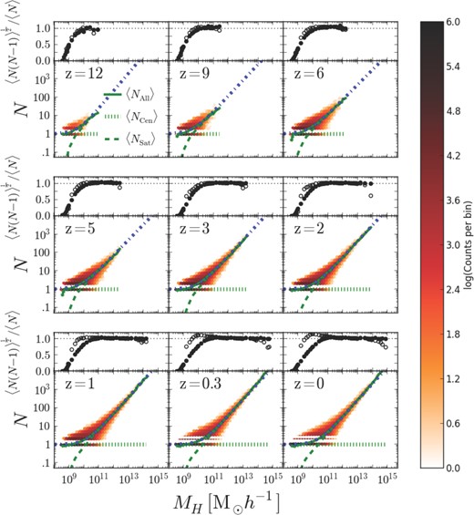
Occupation number and scatter of subhaloes as a function of halo mass. The colour corresponds to the log of the grid density at each occupation number and halo mass. The green over plotted curves are the mean occupation number of central subhaloes (dotted), satellite subhaloes (dashed), and all subhaloes ( solid). The blue dash–dotted curve is the best-fitting power law of the occupation number through all data points. The top panel for each is the width of the probability distribution for all subhaloes (solid circle) and satellite subhaloes (open circle). For a Poisson distribution, with width would be 1 which is the dotted line.
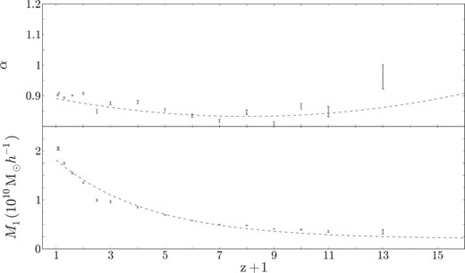
Summary plot of the best-fitting parameters α and M1 as a function of redshift. The green curves are the best fits through each. Table 3 shows the fit functions used and the best-fitting parameters through these fits.
Best fits for the evolution of the power-law index α and normalization mass M1 for increasing redshift.
| Function | A | B | C |
|---|---|---|---|
| α = A + B(z + 1 − C)2 | 0.84(2) | 0.003(1) | 5.4(1.3) |
| M1 = A + Be−C(z + 1) | 0.2(1) | 2.4(2) | 0.34(3) |
| Function | A | B | C |
|---|---|---|---|
| α = A + B(z + 1 − C)2 | 0.84(2) | 0.003(1) | 5.4(1.3) |
| M1 = A + Be−C(z + 1) | 0.2(1) | 2.4(2) | 0.34(3) |
With the best-fitting functions given in Table 3, one could determine the normalization mass M1 and power-law index α at a given redshift, then use equation (7) to determine 〈N〉 in order to populate a given halo of mass Mhalo for a simulation. However, in order to fully populate said haloes, one must also understand the spread of the subhalo population at a certain value of 〈N〉. The best technique for this analysis is to compare the probability distribution of subhaloes N at a given average occupation number 〈N〉, P(N|〈N〉), with that of a well-defined probability distribution, more specifically a Poisson distribution (e.g. Berlind et al. 2003; Zheng et al. 2005). If P(N|〈N〉) follows that of a Poisson distribution, then one could use Poisson statistics to quantize the spread of occupation number from the mean. The top panels of Fig. 6 show the width of the distribution; for a Poisson distribution the width is 〈N(N − 1)〉 = 〈N〉2 which is shown as the dotted line at unity. The solid circles show the width of the probability distribution as a function of Mhalo for all galaxies (both central and satellite). At all redshifts, this distribution is sub Poisson for low values of Mhalo; however, it quickly approaches Poissonian at larger Mhalo. Because the number of central galaxies follows a step function, there is very little spread in this value, i.e. it is either 0 or 1, so instead of exploring the probability for all subhaloes we focused on the probability distribution of satellite subhaloes P(NSat|〈NSat〉). The open circles in the top panels of Fig. 6 show the width of the probability distribution as a function of Mhalo. Again for low halo masses, P(NSat) is sub Poisson, but approaches a Poissonian width for higher masses. On the other hand, for extremely high halo masses at low redshifts, P(NSat) again is sub Poisson. From the width of the distribution, it appears that P(NSat) is very close to a Poisson distribution. In Fig. 8, we plotted P(NSat|〈NSat〉) for three different snapshots. Each plot shows the probability that a halo Mhalo will host NSat satellite galaxies if on average the halo occupation number is 〈NSat(Mhalo)〉. In Fig. 8, the error bars are Poisson error bars and the dotted histogram is the Poisson distribution centred at 〈NSat〉 which is given in the top right of each set of plots. At larger 〈NSat〉, we find that the peak of the distribution is lower in amplitude compared to the Poisson distribution, the width and location of the peak are unchanged though. From Fig. 8 and the top panels of Fig. 6, it is clear that P(NSat|〈NSat〉) can be approximated as a Poisson distribution; therefore, one can adequately use Poisson statistics to quantify the spread of subhaloes from the best-fitting mean of equation (7).
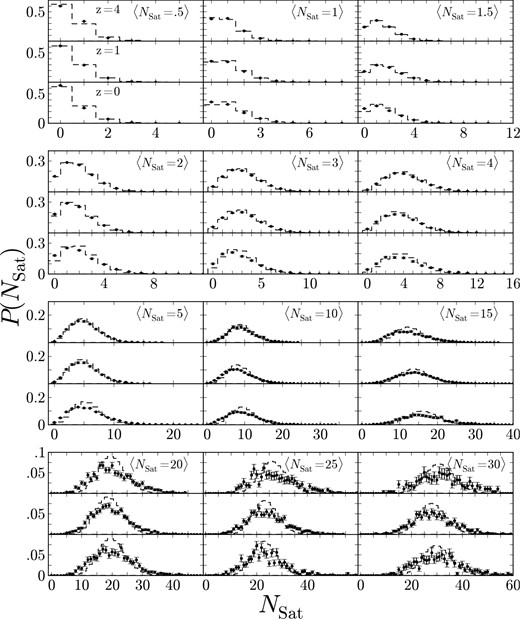
Probability distribution P(NSat|〈NSat〉) for a halo with virial mass Mhalo and an average occupation number of 〈NSat(Mhalo)〉 will host NSat galaxies. Each plot is the distribution about a different value for 〈NSat〉 which is given in the top right, while the three panels correspond to the three redshifts given in the first plot. The error bars shown are Poisson error bars. For comparison the dotted histogram is the corresponding Poisson distribution centred about NSat. Each of the distributions can be very accurately approximated as a Poisson distribution.
Now that we understand the mean occupation number for a halo at a certain redshift, we must also analyse the relative spatial distribution of the subhaloes within their parent halo. As we discussed above, all subhaloes can be classified as either central or satellite; furthermore, each halo will host either one or none central subhaloes, so studying the relative spatial distribution of a central subhalo is a bit trivial, i.e. if the halo hosts a central subhalo it will be located in the centre of the halo. Therefore, we will focus on analysing the spatial distribution of only satellite subhaloes. Fig. 9 shows a simplified 2D schematic of three different haloes of mass Mhalo ∼ 1012 M⊙ h−1 at z = 0 which is comparable to the Milky Way. The middle panel shows a halo with an occupation number equal to the mean at Mhalo (see equation 7), while the left- and right-hand panels show, respectively, the haloes with the minimum and maximum occupation number at Mhalo. The red dotted circle shows the virial radius of the parent halo, the black solid circle shows the virial radius of the central subhalo, and the blue circles show the satellite subhaloes. Because the virial radius of a galaxy is depended on the mass of the galaxy, the size of the circle also represents the mass of each galaxy. This simplified representation easily shows the distribution of mass within each halo; the majority of the mass is located in one large subhalo located at the centre of the group with many less massive galaxies scattered around the central subhalo. Furthermore, this simple schematic shows that the subhaloes prefer to populate their parents haloes along filaments which is roughly shown as the blue dotted line in Fig. 9.
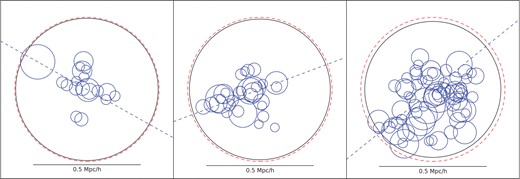
Plotted here is a simplistic schematic of the distribution of sub haloes within three groups of mass Mhalo ∼ 1012M⊙h−1. The left-hand panel shows a group with the fewest number of subhaloes from our simulation, the centre panel shows a group with an occupation number equal to 〈NSat〉 given by equation (7), and the right-hand panel shows a group with the largest number of subhaloes from our distribution. The red dotted circles map out RVir of the parent halo, while the black and blue circles show RVir of the central and satellite subhaloes, respectively. Subhalos are believed to live upon filamentary structures within groups so the blue dotted line roughly shows the filaments of each group.
In Fig. 10, we have plotted (solid curves) the probability density |$\mathcal {P}_{R/R_{{\rm Vir}}}$| that a satellite subhalo will be located a radial distance R from the centre of the group in units of the halo's Rfir. We chose to only investigate satellite galaxies here because we have already shown that haloes can only host one central galaxy which would lead to a trivial analysis. We plotted haloes from three different snapshots while each panel corresponds to different parent halo mass bins. In the last two panels (the high mass panels), there are no haloes with mass 1013 < Mhalo < 1014 at z = 4, so there is no data from that snapshot plotted in these panels. For completeness, plotted on the right-hand axes are the corresponding dotted curves of 〈NSat〉 as a function of radial distance scaled by R200 for each snapshot. Here, 〈NSat〉 is the average number of satellite subhaloes per group per radial bin. In other words, this value corresponds to the average number of satellite subhaloes within a group at a certain radial distance R, which is not the average number of satellite subhaloes withinR. Also plotted as the black curve plotted in the last two panels are SPH data from Berlind et al. (2003). Our distribution follows the same general form as Berlind et al. (2003). As can be seen in Fig. 10 the peak and width of the radial distribution of satellite galaxies decreases with decreasing redshift, irrespective of the mass of the parent halo. This suggests that with time satellite galaxies cluster strongly around the central galaxy and that mergers dominate over the accretion of new satellites. Additionally, we see a mild variation for the peak of the distribution with the mass of the host halo at a given redshift. The relative location of the peak (with respect to Rvir) decreases with increasing halo mass which suggests that the clustering of satellite galaxies is stronger in more massive haloes.

The solid curves here are the probability distribution |$\mathcal {P}_{R/R_{{\rm Vir}}}$| that a satellite subhalo will be located at a radial distance R from the centre of the parent halo in units of the parent halo's RVir. Each panel corresponds to a parent halo mass bin which is given in the right-hand corner of each panel. The colours of the curves correspond to a specific redshift which is given in the top-left corner of the first (top left) panel. The dotted curves correspond to the occupation number 〈NSat〉 at a certain radial distance from the centre of the parent halo. In the last two panels, the black curves show the SPH results from Berlind et al. (2003).
A more detailed comparison between MBII, MBII-DMO, previous work and observations will be presented in a forthcoming paper (Tucker et al., in preparation).
6 GALAXY CLUSTERING
The MBII simulation is of a large enough volume that galaxy clustering can be studied meaningfully. The sheer number of galaxies in the MBII (particularly for low-mass selection thresholds) means that clustering measures can be computed with a high signal-to-noise level and consequently subtle features be noticed and analysed. In this section, we concentrate on two-point correlation functions of the galaxies and dark matter, including the cross-correlation of the two.
6.1 Two point correlation functions
We analyse 15 snapshots of the simulation between redshifts z = 10 and 0.06. For each snapshot, we compute the two-point autocorrelation of dark matter particles and also the two-point autocorrelation function of subhaloes. For the latter, we measure this quantity for several subsamples defined by a lower limit on the subhalo mass: mtot > 109 M⊙, 1010 M⊙, 1011 M⊙, 1012 M⊙. We also do the same for subsamples defined by lower limits on the stellar mass of subhaloes: m* > 108 M⊙, 109 M⊙, 1010 M⊙, 1011 M⊙. We also compute the cross-correlation of dark matter and subhaloes for subsamples defined by the above mass bins.
We note that before computing the correlation functions for any sample in the simulation, if the number of elements (dark matter particles or subhaloes) is greater than 2563, for speed we randomly subsample down to this number, as shot noise errors on the scales we are interested in will be negligible at the sampling density.
In Fig. 11, we show examples of the autocorrelations and cross-correlations for galaxies and dark matter in the MBII at two redshifts, z = 0 and 2. In this example, the galaxies used to compute the clustering were selected above a stellar mass threshold of 108 M⊙. There were 3.82 × 10⁵ galaxies in the subsample at z = 0 and 5.67 × 10⁵ at z = 2. In Fig. 11, we can see that the dark matter autocorrelation (referred to as ξρρ although it is not the autocorrelation of the total density) at z = 0 has the pronounced dip at r ∼ 1 h1 Mpc indicating the transition between one-halo and two-halo terms (Cooray & Sheth 2002). At redshift z = 2, the autocorrelation of galaxies and of dark matter particles have similar shapes and amplitudes on scales r > 20 kpc h−1, but at z = 0 the galaxies (which have low mass) are significantly antibiased with respect to the dark matter on all scales (see e.g. Abbas & Sheth 2007). The cross-correlation, ξgρ has a second dip in it at r ∼ 20 kpc h−1.
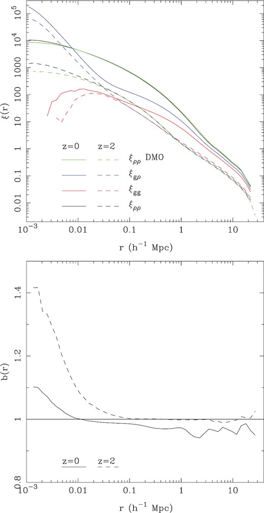
Top: the two-point autocorrelation function of dark matter from MBII (black) and MBII-DMO (green), galaxies (red) and the two-point cross-correlation function of dark matter and galaxies (blue) in the MBII simulation. We show results at two redshifts z = 0 and z = 2. The galaxies were selected to be those above a stellar mass threshold of 108 M⊙. Bottom: relative bias of DM in the MBII run compared to the MBII-DMO run, |$b(r)=\sqrt{\xi _{\rho \rho }/{\xi _{\rho \rho -{\rm DMO}}(r)}}$|.
In Fig. 11, we also show the autocorrelation function of the dark matter distribution in the MBII-DMO simulation, ξρρ − DMO. Comparing this to ξρρ for the MB-II run, we are able to see the effect that baryonic physics has on the clustering of dark matter. From the upper panel, we can see that the shapes are very similar. Dividing one curve by the other enables us to see any small differences, and this is done in the bottom panel, where we plot the relative bias of the MBII autocorrelation function compared to that of MBII-DMO, i.e. defined by |$b(r)=\sqrt{\xi _{\rho \rho }/{\xi _{\rho \rho -{\rm DMO}}(r)}}$|. We find that below 10 kpc h−1 at z = 0 and 100 kpc h−1 at z = 2 baryonic physics causes a boost to clustering in the dark matter, by up to 40 per cent in |$\sqrt{\xi _{\rho \rho }}$| on the smallest scales plotted. We also find that a relative bias of 1 larger scales than ∼ 100 kpc h−1 at redshift 0 but that at redshift 2 there is a ∼2 per cent suppression of power on large scales with respect to the DMO run.
6.2 Bias and stochasticity in MBII
6.2.1 Bias
That the ratio of dark matter and galaxy correlation functions can vary as a function of scale is obvious from Fig. 11. In Fig. 12, we plot |$b(r)=\sqrt{\xi _{gg}(r)/\xi _{\rho \rho }}$| for the same lower stellar mass threshold m* ≥ 108 M⊙ as was used in Fig. 11, but for redshifts between z ∼ 0 and z ∼ 10. The b(r) function is approximately flat for separations r > 2–5 h1 Mpc, depending on the redshift, reaching the limit on large scales usually referred to as linear bias (see e.g. Scherrer & Weinberg 1998). On smaller scales, the bias is scale-dependent, with bias decreasing as r becomes smaller for redshifts z < 4 and increasing for redshifts z > 4. For the mass threshold plotted, bias is approximately scale-independent at z = 4 down to r ∼ 0.1 h1 Mpc. The scale dependence at late times is presumably due at least partly to non-linear effects such as merging of galaxies reducing the number of pairs on small scales, as well as halo exclusion. In the halo model framework, bias is scale-dependent with a change of slope at the transition scale between the one and the two halo terms. At earlier times, because we are using a fixed threshold mass, the galaxies become rarer and so are likely to lie in primary haloes (i.e. they are not in subhaloes of larger haloes).
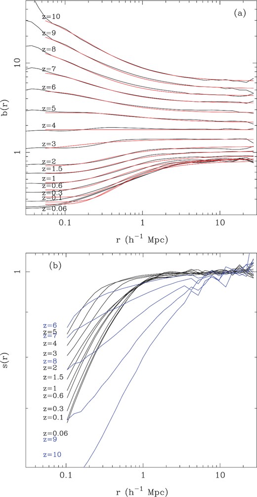
(a)Top panel: bias versus scale for galaxies in the MBII simulation, at 15 different redshifts. The lower threshold mass of the MBII galaxy sample was chosen to be 108 M⊙. The simulation results are shown as solid black lines, and a simple parametric fit (Equation 8) to the results for each redshift is plotted as a solid red line. (b)Bottom panel: stochasticity of galaxy clustering (equation 10) as a function of scale for MBII galaxies. The same threshold mass (108 M⊙) was used as in the top panel and the same redshift snapshots. In order to make the redshift progression clearer, we plot results at redshifts above z = 5 with blue lines and the low-redshift results in black.
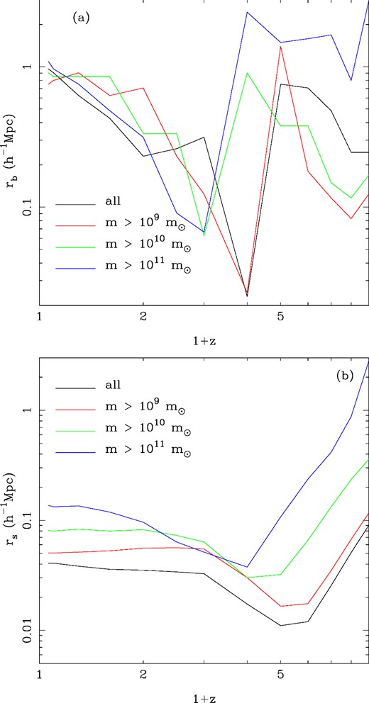
(a)Top panel: the non-linear scale in the bias (parameter rb in equation 8) of MBII galaxies as a function of redshift. We show results for four different lower (total) mass thresholds as different coloured lines. (b) Bottom panel: the non-linear scale in the stochasticity (parameter rs in equation 10) of MBII galaxies as a function of redshift. We show results for the same four different lower (total) mass thresholds as the top panel.
We note that in Fig. 12(a) that for the subhalo mass sample we are plotting the values of blarge and bsmall in the fits will change relative to one another as we change redshift. As a result there will be a redshift (for this mass subsample it is around redshift z = 3–4) where the bias will be almost linear (blarge ≃ bsmall). There is also likely to be a transition in the non-linear scale parameter rb at around this redshift.
In Fig. 13(a), we plot the behaviour of rb versus redshift, with results for several different mass bins on the same plot. At low redshifts z < 2, we can see a gradual increase in rb with redshift for all mass subsamples. This non-linear scale reaches a maximum of 1 h−1 Mpc at z = 0. This can be compared to the scale at which matter clustering becomes non-linear (the matter clustering deviates from the linear extrapolation), which is ∼5 h−1 Mpc at this redshift (Gaztañaga & Juszkiewicz 2001). Galaxies therefore trace the mass to scales significantly smaller than the non-linear mass clustering scale in this simulation.
The minimum value for rb is reached at redshift z = 2 and is between rb = 0.01–0.05 h−1 Mpc with the smaller haloes being at the lower end of this range. At earlier redshifts, there is then a switch to a much larger value for rb.
6.2.2 Stochasticity
6.3 Comparison with observations
We compare first to the galaxy autocorrelation function published by the VIMOS Public Extragalactic Redshift Survey (VIPERS) team (Marulli et al. 2013). The VIPERS survey is an ongoing deep and well-sampled spectroscopic survey of 100 000 galaxies in the redshift range z = 0.5–1.2 (see Guzzo et al. 2014 for details). We use two of the three redshift bin measurements published by Marulli et al. (2013), centred at z = 0.6 and 1.0. Marulli et al. (2013) give the linear bias parameter for each redshift in a series of bins in stellar mass threshold (their table 3). We plot these linear bias versus stellar mass points in Fig. 14. Results from the simulation are shown as lines (b in this case is the parameter blarge fit using equation 8). From Fig. 14, we can see that the simulation and observations show the expected trend of increasing bias with increasing galaxy stellar mass, and that the simulations are consistent with the observational results.
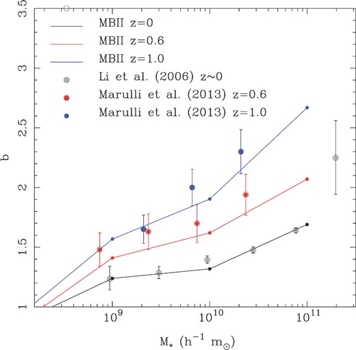
Top panel: linear bias versus threshold galaxy stellar mass. Results for galaxies in the VIPERS survey (Marulli et al. 2013), are shown as points with error bars, at two different redshifts, z = 0.6 and 1. Results from the SDSS at low redshift (Li et al. 2006) are also shown. We show results from the MBII simulation at the same redshifts as solid lines.
As the MB-II simulation reaches z ∼ 0, it is also interesting to compare to a sample from the wide range of observational data at the lowest redshifts. In Fig. 14, we plot the b versus stellar mass relationship from the simulation at z = 0. We also show results from the SDSS (Li et al. 2006) measured from 200 000 galaxies in the SDSS main galaxy sample. The observational results were presented in terms of relative bias between galaxies at the knee of the stellar MF (characteristic stellar mass M* = 4.11 × 10¹⁰ M⊙) and other stellar mass bins. Before plotting, we have converted this bias into a relative bias between dark matter and galaxies by using the value of b measured in the MB-II simulation at this stellar mass scale. We can see that the variation of b with stellar mass in the observational data and simulation are consistent.
Observationally analyses such as Jullo et al. (2012) have been able to probe scale dependence of bias by comparing weak-lensing measurements of the matter distribution with galaxy clustering. In Fig. 15, we show a quantitative comparison between the MBII simulation and the data from fig. 11 of Jullo et al. (2012). The Jullo et al. (2012) measurements were for five different subsamples of observed galaxies with different mean stellar masses and mean redshifts. In order to match the mean stellar masses and redshifts of the Jullo et al. (2012) data samples, we carried out a quadrilinear interpolation in log mass and in redshift between the correlation function results measured from the MBII simulation for different redshift snapshots and mass bins. The relevant redshifts and mean stellar masses for the different samples are given in the panels of Fig. 15.
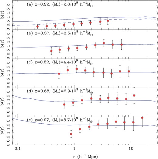
The scale dependence of bias in the MBII simulation (blue lines) compared to the observational data of Jullo et al. (2012, points with error bars) for various samples with different mean stellar mass and redshift (given in the panels). The dashed line in panel (a) shows the results for an MBII sample with a mean stellar mass of 1.5 × 10⁹ M⊙.
Looking at Fig. 15, we can see that observed data does show a pronounced antibiasing (b < 1) of galaxies with respect to dark matter on small scales for many of the galaxy subsamples. For the lowest redshift subsample (top panel) this is particularly significant, given the small error bars. The MBII simulation data exhibits this trend also, for the bins with low mass and low redshift. The bias for the lowest redshift bin is systematically higher at all scales in the simulations compared to the observations, however. In order to show quantitatively how this relates to the mean stellar mass of the subsample, for this panel, (a), we have also plotted the results for a subsample with approximately half the mean stellar mass (1.5 × 10⁹ M⊙).
Jullo et al. (2012) have also searched for for stochasticity in clustering by comparing weak-lensing measurements of the matter distribution with galaxy clustering. Jullo et al. (2012) find no significant amount of stochasticity on scales between r = 0.2 h1 Mpc and r = 15 h1 Mpc at redshifts between z = 0.2 and 1.
A comparison between the MBII simulation results and those of Jullo et al. (2012) is shown in Fig. 16. The observational points are for a range of redshifts, with each redshift's measurement being reliably inferred over a particular range of scales (shown by the horizontal error bars). The different observational points also came from different flux limited samples, which have a mean stellar mass varying between 6 × 10⁹ and 1.8 × 10¹⁰ M⊙ h−1. We can see that the observational results are all consistent with no stochasticity (s = 1) at at least the 1.5σ level. The simulation results are shown for redshifts and stellar mass ranges which bracket the observational results. We can see that the observational and MBII results are consistent, but at the scales r > 0.4 h1 Mpc that are probed by Jullo et al. (2012) we expect no significant deviation from s = 1. On smaller scales for the MBII, we see differences between the two samples of different masses. The galaxy-exclusion effect mentioned above means that s(r) goes above 1 at smaller scales for smaller galaxies.
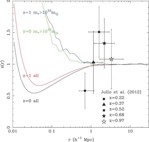
Stochasticity versus radius. Results for different redshifts and mass thresholds in the MBII simulation are shown as coloured lines. The points with error bars denote observational determinations for galaxy stochasticity by Jullo et al. (2012). The simulation redshifts and mass bins shown bracket those of the observational data.
7 PROPERTIES OF GALAXIES
The MB and MBII simulations have been very successful in reproducing the observed properties of galaxies in the high-redshift Universe. Wilkins et al. (2013a) showed that the GSMF predicted by MB and MBII at z ≥ 5 could be reconciled with observations if one assumed that the mass-to-light ratio (as predicted in MB and MBII) of these galaxies was evolving with redshift. Khandai et al. (2012) showed that the MB simulation reproduced the observed properties of galaxies hosting the highest redshift quasars (Carilli et al. 2007; Wang et al. 2010, 2011). In this section, we focus our attention on the properties of galaxies in the MBII simulation at z < 4. We will compare general properties of galaxies with observations and leave a detailed analysis to future publications.
We start by looking at the cosmic spectral energy distribution (CSED) in MBII. We select subhaloes using SUBFIND and consider only those which have more than 100 dark matter particles. We refer to these subhaloes as galaxies for the rest of this section. The SED of a galaxy is generated by summing the SEDs of each star particle in the galaxy. The left- and right-hand panels of Fig. 17 show the evolution of the CSED in the MBII simulation from z = 10 to 0. We find that the amplitude of CSED in all bands increases rapidly with decreasing redshift to z = 4 with little change in shape. This is expected and is in line with the behaviour of the observed cosmic star formation rate (CSFR, see Fig. 23). Observations find that the CSFR plateaus around z ∼ 3–4 and declines rapidly at lower redshifts.
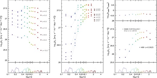
The Evolution of the CSED in MBII (left-hand and centre panels. Comparison is made at z = 0.0625 with the GAMA survey at z = 0.05 (Driver et al. 2012).
The shape of CSED evolves dramatically below z ≲ 3. We find that the bluer part of the CSED, which strongly correlates with the CSFR starts to decline below z ≲ 3 consistent with the observational trend, whereas the redder part of the CSED increases very slowly with decreasing redshift to z ∼ 1 and declines thereafter. This is because at these redshifts galaxies are forming new stars at much reduced rates and are passively evolving into a redder population.
In the right-hand panel of Fig. 17, we compare the intrinsic CSED at z = 0.0625 with dust-corrected observations from the GAMA survey at 0.013 < z < 0.1 (Driver et al. 2012). We find that the shape of the CSED compares well with the observational results. However, the amplitude of the CSED predicted by MBII does not match that of observations, falling systematically below it. This will be in part caused by incompleteness as MBII does not resolve all galaxies (particularly those at low stellar masses).
This discrepancy is also sensitive to the IMF assumed in the processing of MBII e.g. the Salpeter IMF. Assuming a Chabrier IMF in which a larger fraction of the mass is converted into high-mass stars (such as those proposed by Kroupa 2001; Chabrier 2003) would increase the luminosity density by a factor of ∼2 (which is still short of the factor of ∼3 compared to GAMA) bringing MBII more closely inline with the observations. The GAMA points are constructed from the individual luminosity functions which are integrated to zero and should therefore account for all galaxies in the Universe. We have tested that if we include all star particles in the simulation the amplitude of the CSED is enhanced by 0.1 dex therefore resolving smaller galaxies and using a Chabrier IMF should improve the normalization of the CSED.
We now look at the GSMF predicted in MBII in Figs 18 and 19. In Fig. 18, the GSMF is compared with observational estimates. The black line represents the GSMF in MBII when we consider all galaxies. The red, green, blue and cyan lines denote the population of galaxies which have an SFR greater than 0, 0.01, 0.1. and 1, respectively (in units of M⊙ yr−1.) We have also added the GSMF (pink line) from simulations of Hirschmann et al. (2014). Comparison is made with observations of Pérez-González et al. (2008, grey data points), Baldry et al. (2012, orange data points – z=0). For z = 2 and 3 (orange data points), the observational estimates are taken the CANDELS survey (Tomczak et al. 2013). At z = 0, MBII overpredicts the GSMF both at the high- and low-mass ends. However, the GSMF agrees well with the observations for M* ≥ 1010 M⊙ h−1 for z = 1 and 2. At z = 3, MBII underpredicts the abundance of larger mass galaxies. This is most likely due to the finite volume of MBII.
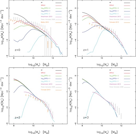
The GSMF from z = 0–3 in MBII. Comparison is made with recent simulations of Hirschmann et al. (2014, pink line) and observational estimates of Pérez-González et al. (2008, grey data points with error bars), Baldry et al. (2012, z=0, orange data points with error bars). For z = 2 and 3 (orange data points with error bars) the observational estimates are taken the CANDELS survey (Tomczak et al. 2013). The black line represents the GSMF in MBII when we consider all galaxies. The red, green, blue and cyan lines denote the population of galaxies which have an SFR greater than 0, 0.01, 0.1. and 1, respectively (in units of M⊙ yr−1.)
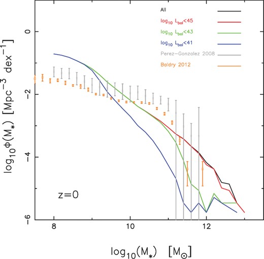
Same as in Fig. 18 but we now consider the population of galaxies at z = 0 which may host an AGN with bolometric luminosity, log10(Lbol) < 45 (red), log10(Lbol) < 43 (green) and log10(Lbol) < 41 (blue).
We find that the amplitude of the GSMF of Hirschmann et al. (2014) is larger compared to MBII although the shape seems to be in reasonable agreement. The boxsize, star formation and feedback model in MBII and Hirschmann et al. (2014) are similar. Therefore given that the mass resolution of Hirschmann et al. (2014) is ∼ × 60 lower than MBII and based on the resolution tests carried out in Torrey et al. (2014) the amplitude of the GSMF in Hirschmann et al. (2014) should be lower compared to MBII.
One of the striking feature at all redshifts is the steep slope in the GSMF in MBII at M* ≤ 1010 M⊙ h−1. These galaxies are less affected by AGN feedback and are therefore more sensitive to the star formation and stellar feedback model. This feature is seen across all redshifts in Fig. 18. For example in MBII, we find that there are many more lower mass galaxies which have zero star formation (i.e. the difference between the black and red lines) at z = 0 as compared to higher redshifts, the difference between the two decreasing with increasing redshift. We therefore need to understand why do small galaxies form rapidly so early and why do they stop forming stars later. A better treatment of the star formation and stellar feedback model is therefore required in order to suppress the overproduction of lower mass galaxies. For example our model does not include the treatment of molecular gas (Krumholz & Gnedin 2011) which would tend to suppress SFRs in lower mass galaxies. Alternately, one may need to assume a feedback model which is dependent on the mass of the galaxy (Oppenheimer & Davé 2006; Davé, Oppenheimer & Finlator 2011; Vogelsberger et al. 2013; Torrey et al. 2014). The variable wind model which is dependent on the galaxy velocity dispersion is described in Oppenheimer & Davé (2006) and indeed flattens the GSMF at z = 0 better reproducing observations. However, Torrey et al. (2014) find that the GSMF is still steep at higher redshifts and additional modelling may be required to suppress the production of stars in low-mass galaxies. Interestingly, we find that if we account for those galaxies which have non-zero star formation at z = 0, the lower mass end of the GSMF is in better agreement with observations.
In Fig. 19, we look how the AGN population affects the GSMF at z = 0. We consider the population of galaxies which may host an AGN with bolometric luminosity in units of erg sec−1, log10(Lbol) < 45 (red), log10(Lbol) < 43 (green) and log10(Lbol) < 41 (blue). We focus our attention on larger mass galaxies at z = 0 since they are most affected by AGN feedback. This figure shows that bright AGNs are systematically hosted in more massive galaxies. We find that the tail of the GSMF is in reasonably good agreement with observations down to z ≥ 1 (see Fig. 18) and one does not need to consider a subsample of galaxies without bright AGNs (green and blue curves) to match observations. We find that the stellar mass in galaxies that host AGNs brighter than log10(Lbol) = 43 is overpredicted in MBII. Similar to the BH accretion rate for the most massive BHs at z = 0 (see the discussion in the next section), we find that the massive galaxies have very high SFRs and the mechanism to quench star formation through AGN feedback is not sufficient at low redshifts for these objects. This is also seen in the results of Hirschmann et al. (2014).
Recent hydrodynamic simulations (Vogelsberger et al. 2013; Torrey et al. 2014) with the arepo code (Springel 2010) on the other hand reproduce the tail of the GSMF reasonably which may be a result of missing cluster sized haloes in their simulation volume of Lbox = 25 Mpc h−1. However, when these simulations were scaled to larger volumes of Lbox = 75 Mpc h−1, e.g. in the Illustris simulation (Genel et al. 2014; Vogelsberger et al. 2014a,b), the GSMF is still overpredicted at large masses at z = 0. Similar predictions are also seen in the results of Bachmann et al. (2015) which attempt to refine the accretion and feedback models of BHs in this work.
Simulations from the EAGLE project (Schaye et al. 2015), which are comparable in volume and resolution to MBII and were also run with gadget3, reproduce the GSMF extremely well since they calibrated the feedback efficiencies from massive stars and AGNs to the present-day GSMF, the amplitude of the MBH–σ relation and galaxy sizes. For example they employ a value of the feedback energy parameter f = 0.15 which is three times that used here. By construction the best agreement to the GSMF is at z = 0.1, however they show that the evolution of the GSMF agrees reasonably well with observations to z = 2 (Furlong et al. 2014). At higher redshifts, the GSMF gets steeper at low masses and underpredicts larger galaxies comparable to what we see in MBII. Given that the tail of the GSMF are comparable in EAGLE and MBII at z = 1 and agree well with observations, one may need to employ a larger feedback energy parameter (comparable) to EAGLE at z < 1 in MBII. It would also be interesting to see the predictions on the BH MF and AGN luminosity functions from the EAGLE project.
Another caveat is the way we define galaxies. Torrey et al. (2014) define the galaxy stellar mass to be the sum of the stellar mass within twice the half-mass radius. Such a definition affects only larger objects as it gets rid of the stellar mass in the diffuse intracluster medium and is not traditionally counted as contributing to the central galaxy's mass. Such a definition may help in better bringing in line our results with observations but as we will discuss in the next section the bright end of the QLF is still overestimated due to insufficient AGN feedback.
8 BLACK HOLES
In this section, we present some basic properties of our simulated BH population and their relation to the galaxies in MBII. In particular, we show overall history of the BH mass assembly and look at the relation between BH and stellar mass in galaxies. We look at the predictions for the bolometric luminosity function and clustering strength as a function of luminosity for the AGN population in MBII. More detailed analysis of the BH–galaxy relations and comparisons with observational constraints will be presented in a separate paper.
Every single BH in our simulations accretes and grows according to local gas properties so as an outcome of our BH model, each single BH that has a light curve and an associated mass history over the cosmic time since it is seeded. MBII contains tens of thousands of BHs and Fig. 20, we show the mean (and associated dispersion, in the corresponding coloured areas) BH mass assembly history for BHs that, at z = 0, end up in different mass bins, from the lowest masses (106 M⊙ h−1 < MBH < 107 M⊙ h−1) to the highest mass bin (109 M⊙ h−1 < MBH < 1010 M⊙ h−1). In addition to the mean histories for the population, we also specifically show a sample of single, main progenitor mass assembly histories. This is to illustrate how the most massive, and earliest growing BHs, within the different mass bins, depart from the mean (dominated by the more numerous lower mass BHs). In general, we see that the largest BHs z = 0 are largely assembled at high redshifts. The dispersion in mass assembly histories is also typically larger for the high-mass BHs. This is because there is a much larger variety of assembly histories for a large mass progenitor than for the lower mass progenitor. For example, some BHs form early and grow to large masses quickly at high-z, but their mass assembly history remains flat subsequently. We also note an upturn in the growth histories of massive BH at z < 1. This is likely the result of insufficient AGN feedback (in the form that is modelled in MBII) in massive galaxy hosts at low redshift. Similar results were also found by recent work of Hirschmann et al. (2014).
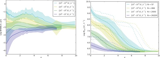
The mean BH accretion rate (left-hand panel), excluding mergers and the mean BH mass assembly history for the main progenitor (right-hand panel) BHs ending up in different mass ranges (as labelled) at z = 0. N indicates the number of BHs in each of the mass bins. The dashed and dotted lines show a sample of single main progenitor histories.
The growth (including mergers) of the most massive BHs that end up as 109–1010 M⊙ h−1 BHs at z = 0 is dominated by gas accretion. The total mass gained via mergers for the most-massive-progenitor histories of the 57 BHs that end up in the 109–1010 M⊙ h−1 mass bin gain a total of 2.5 × 10¹⁰ M⊙ h−1 from mergers (which translates to 20 per cent of the total z = 0 mass of these BHs) of which 75 per cent (1.89 × 10¹⁰ M⊙ h−1) of the mass gained by mergers is below z = 1. Therefore, growth of these massive BHs is dominated by gas accretion. Additionally, we found that for the mass gained through mergers below z = 1 for those 57 BHs, 30 per cent comes from just three BHs, and those BHs are not the most massive BHs at the end of the run (in terms of mass they are ranked 2, 6, 10 in the mass range 109–1010 M⊙ h−1 the specified mass range). So the median (rather than mean) fraction of growth via mergers is going to be lower.
To illustrate the range of BH masses and luminosities in MBII, we show these two quantities as a function of total halo mass in our galaxies in Fig. 21. Although there is an overall correlation between both quasar luminosity and BH mass with halo mass, the scatter in both these relations is rather large indicating the halo mass is an extremely rough proxy to BH properties. Complex hydrodynamic and associated feedback effects play an important role in the central region of galaxies.
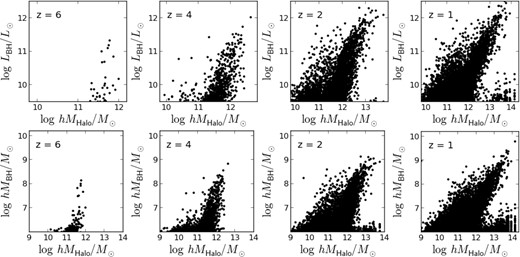
The relation between BH luminosity and host halo mass (top) and BH mass and host halo mass (bottom).
In the top panel of Fig. 22, we show the z ∼ 0 prediction for the relationship between BH mass and stellar mass in galaxies in our simulation. Instead of a scatter plot, we show the contours that correspond to the 1σ, 2σ and 3σ population of points in the MBH–M* plane. Due to limited resolution, we are unable to resolve the stellar-bulge of the lower mass galaxies. Additionally, we find that an often used proxy for bulge mass, i.e. the mass enclosed within twice the half-mass radius as in Sijacki et al. (2014) only affects larger mass objects. Therefore for simplicity here we use the total stellar mass and not only the bulge mass which is what is normally used in the local universe (in future work we will look at the associated BH–stellar velocity dispersion relation).
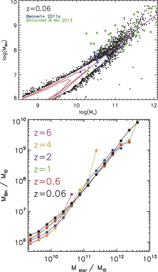
Top: present-day BH mass stellar mass relation in MBII. The contours correspond to the 1σ, 2σ and 3σ population of points in the MBH–M* plane. The black data points are again from MBII but lie outside the 3σ population. Data points are from Bennert et al. (2011, blue) and McConnell & Ma (2013, green). The line is the observational constraint from Häring & Rix (2004). Bottom: the evolution of the MBH–M* relation in MBII.
The black data points are again from MBII but lie outside the 3σ population. We compare our results with observations by (Bennert et al. 2011, blue) and (McConnell & Ma 2013, green). The line is the observational constraint from Häring & Rix (2004) and we find good agreement between our results and observations. However observationally the scatter at high masses seems to be larger than MBII.
In the bottom panel of Fig. 22, we show the evolution of the mean relation derived from a number of snapshots from MBII consistent with previous work (Di Matteo et al. 2008; Booth & Schaye 2011; Hirschmann et al. 2014). Although we do not find strong evolution in the relation with redshift, the relation appears to steepen slightly towards higher redshift. This is overall consistent with previous findings and observational constraints (Bennert et al. 2010; Merloni et al. 2010) and we defer a detailed comparison with different observational constraints as a function of redshift to a future paper (Degraf et al., in preparation).
The global SFR and BH accretion rate density (multiplied by a factor of 3 × 10³) is shown in Fig. 23 together with the observational compilation of Hopkins & Beacom (2006) for the SFR density derived from different wavebands. Overall the SFR and BH accretion rate density have similar shapes and track each, with the peak of star formation proceeding that of BH accretion rate (BHAR) density by roughly a unit redshift. Both the SFR density (and also the BHAR density) show a flattening below z ∼ 1. This is likely a result of too inefficient feedback to quench both SFR and BHAR in low-redshift high-mass haloes.
The SFR (in red) and BHAR (in orange, multiplied by 3 × 10³ for comparison) density prediction from MBII. The observation constraints for the SFR density from Hopkins & Beacom (2006) are shown in grey squares (without error bars for clarity).
In Fig. 24, we show the bolometric QLF compared to the compilation of data from Hopkins et al. (2007), at z = 0.1, 0.5, 1, 1.5, 2 and 4. The central line in each panel is the MBII prediction for the bolometric QLF compared to the Hopkins et al. (2007) data compilation at different redshifts. The upper and lower lines are Poisson error bars of the binned data in MBII. We note that z > 5 predictions from MBII (and MB) are presented in DeGraf et al. (2012) and McGreer et al. (2013), and predictions for z = 2.0, 2.4, 3.2 compared to the most up-to-date BOSS QLF in Ross et al. (2013). In general, we find overall good agreement between the simulations and observations at z > 2 (here and in DeGraf et al. 2012, McGreer et al. 2013 and Ross et al. 2013, and at z = 0.5.) At the lowest redshifts (z = 0.1), however, the bright end of the QLF is overestimated by the simulations. As we discussed earlier in the section, this indicates insufficient quenching/AGN feedback at these redshifts. Conversely, in the redshift range between z = 1.5–2, the bright end of the QLF is underestimated (see also Ross et al. 2013). This would indicate that our peak of the BHAR density occurs somewhat too early (see Fig. 23). Again this may have to do with the details AGN feedback. Given the simple model adopted here, these results suggest that a constant f (our feedback energy parameter) may be too simplistic a model for AGN feedback. A redshift evolution of f as also implemented by Hirschmann et al. (2014) may alleviate some of these issues [however, even in those simulations the bright end (at low-z) is overestimated indicating that some more complicated modelling may be necessary].
The central line in each panel is the MBII Predictions for the bolometric QLF compared to the Hopkins, Richards & Hernquist (2007) data compilation at different redshifts. The upper and lower lines are Poisson error bars of the binned data in MBII.
Finally, we briefly present the MBII prediction for the correlation length, r0 of AGN as a function of redshift and luminosity cut in Fig. 25. We plot r0 measured for different quasar populations (lines top to bottom are for L/L⊙ > 1011, 1010, 109) as a function of redshift. With an increasing luminosity cut in MBII, the sample gets smaller and the error bars get larger.
The correlation length, r0 measured for different quasar populations (lines top to bottom are for L/L⊙ > 1011, 1010, 109) as a function of redshift.
In general, the correlation lengths are in agreement with observational constraints (Shen et al. 2009) at low redshifts. However due to the relatively small volume in MBII, we are not able to probe the bright end of the quasar population at high redshifts which leads to lower clustering in comparison to observations.
The correlation length at a fixed luminosity cut, increases as a function of redshift. This is expected if same luminosity AGN are hosted in similar mass haloes at different redshifts. In addition, there is a luminosity dependence in the clustering and r0 increases by a factor of 2–3 at the highest luminosities.
9 CONCLUSIONS
In this paper, we have examined a variety of standard predictions using the recently completed MBII simulation. In particular, the results presented here range from the clustering of haloes and galaxies, HOD, the MF of haloes to basic properties of galaxies and AGNs.
Our main conclusions are as follows.
We find that haloes with masses Mhalo ≥ 1013 M⊙ h−1 have a baryon fraction close to 80–90 per cent of the cosmic mean. The baryon fraction decreases steadily with decreasing halo mass. Our results are broadly consistent with Crain et al. (2007) for cluster sized haloes but differ significantly for lower mass haloes. The discrepancy can be attributed to feedback both from AGN and supernovae which were not modelled in Crain et al. (2007).
We find that the FOF halo MF (where halo mass includes both dark matter and baryonic components) in MBII can be fitted with a universal form (valid for all redshifts) at the ∼13 per cent level.
One of the most striking results predicted by MBII is the behaviour of the halo MF which shows a strong suppression in the abundance of haloes below the knee of the MF (ln (1/σ) ≲ −0.2 which corresponds to Mhalo ∼ 1013.2 M⊙ h−1 at z = 0 and Mhalo ∼ 109.5 M⊙ h−1 at z = 3) when compared to DMO predictions of the halo MF. This is due to the significant impact of baryonic processes which tend to suppress the mass of the halo by up to 30 per cent Sawala et al. (2013).
Fits to the MF from DMO simulations overpredict the MF at the 20–33 per cent level below the knee of the MF at ln (1/σ) ≲ 0.2.
When compared to an identical DMO variant, i.e. MBII-DMO, the suppression of the MF in MBII is at most at the 20 per cent level below the knee of the MF.
We have quantified the scale dependence of bias and stochasticity in the simulation. We find that scale of the deviation from a linear fit for both bias and stochasticity reaches a minimum at z ∼ 3–4. The galaxy and mass density field can in this sense be said to trace each other most closely at this redshift.
The MBII overall matches most observed measurements of galaxy clustering with stellar mass. There are however some discrepancies in the bias at the lowest masses and redshifts probed. The simulation is consistent with observed measurements of stochasticity from combinations of galaxy clustering and weak lensing.
We find that the HOD is well described by a power-law behaviour (see equation 7). We find a modest evolution for the power-law slope however the normalization mass for the distribution exhibits an exponentially decaying behaviour with redshift.
The location of the peak and the width for the radial distribution of satellite galaxies decrease with decreasing redshift irrespective of the host mass of the halo, showing that satellite galaxies cluster more strongly around the central galaxy with time.
We find that the shape of the CSED in MBII is consistent with observed data. The amplitude is however much lower and can be attributed to incompleteness at low galaxy masses in MBII.
The GSMF predicted by MBII is consistent with observations out to z = 2. At lower redshifts however the MBII GSMF is much steeper at lower masses whereas MBII over produces stars at larger masses at z = 0.
We find BH mass and AGN luminosity to be broadly correlated to host Mhalo but with very large scatter, indicating a wide range of BH properties for a given halo mass. However, the local MBH–M* relation is tighter and consistent with the observed one. Our results also imply very moderate evolution for the MBH–M* from z ∼ 2. The global SFR density and BH accretion rate density are also similar, but with a peak for the latter shifted to later times.
The bolometric luminosity function of the simulated AGN population is broadly consistent with observational constraints (see also Ross et al. 2013). We note however that simple thermal coupling for AGN feedback appears to quench the bright end of the AGN LF too fast around z ∼ 2 whilst not being sufficient to fully quench the brightest AGN at z = 0. The best agreement with observations is at z > 2 and z ∼ 0.5. Our results show a weak dependence of AGN clustering with luminosity (we defer to future work a detailed analysis of the AGN population).
The MBII simulation is the largest simulation of its kind run to date with sufficient resolution to resolve 109 M⊙ h−1 haloes. We have found that the properties, such as HOD and clustering are consistent with previous work and observations. However, we find that feedback from AGNs is still not sufficient at lower redshifts to properly account for the properties of large galaxies and AGNs since it is unable to quench star formation in massive galaxies and the abundance of luminous quasars. However, it describes the current state of standard SPH simulations of galaxy formation and should be used as a testbed for improving models of galaxy formation. The parameters used in MBII were based on much smaller SPH simulations which missed these large haloes in their volumes and thus could not find discrepancies with observations at the large mass end.
At smaller masses, the GSMF in MBII is very steep compared to observational constraints. A variable wind model based on the galaxy velocity dispersion (Oppenheimer & Davé 2006; Davé et al. 2011; Vogelsberger et al. 2013; Torrey et al. 2014) has been shown to flatten the GSMF at smaller masses to better reproduce observational constraints at z = 0. However at higher redshifts, these models still predict a steep slope. On the other hand, we find that AGN feedback is still insufficient to quench star formation in the most massive galaxies. The effect of AGNs is important in regulating the growth of massive galaxies; e.g. the results of Davé et al. (2011, which do not include AGN feedback) and those of Vogelsberger et al. (2013) and Torrey et al. (2014, which include AGN feedback) clearly illustrate how AGNs affect the stellar content of massive galaxies. However these simulations, still small in volume, miss out on massive haloes but when scaled to larger volumes of Lbox = 75 Mpc h−1, e.g. in the Illustris simulation (Genel et al. 2014; Vogelsberger et al. 2014a,b), the GSMF is still overpredicted at large masses at z = 0. The other approach would be to calibrate the parameters of the subgrid models to match the well-constrained local observables like the GSMF as was done in the EAGLE project (Schaye et al. 2015). In subsequent work, we will look at improving on the feedback models employed in MBII as well as calibrating the parameters of the subgrid models to better match observations.
One of the important effects we have quantified here is the effect of baryonic processes on the halo MF. Although we find that the universality of the MF in MBII holds at the 13 per cent level consistent with previous work, considerable differences exist in the abundance of haloes below the knee of the MF when compared to dark matter simulations. One of the natural questions which arise are: how do different models for star formation, BH growth and feedback affect the MF? How strong is the redshift dependence? What can be said of halo abundance matching techniques and their predictions when done with MFs such as MBII? These questions can only be addressed with simulations with different galaxy formation models and corresponding dark matter simulations which we will address in future work.
The authors would like to thank the anonymous referee for valuable suggestions and comments. The simulations were run on the Cray XT5 supercomputer Kraken at the National Institute for Computational Sciences. This research has been funded by the National Science Foundation (NSF) PetaApps programme, OCI-0749212 and by NSF AST-1009781. This work was partially supported by the National Institute of Science Education and Research, India. The MBII-DMO simulation was run on Hopper of the National Energy Research Scientific Computing Center, a DOE Office of Science User Facility supported by the Office of Science of the US Department of Energy under Contract no. DE-AC02-05CH11231. We would like to thank Katrin Heitmann and Rachel Mandelbaum for letting us complete the MBII-DMO simulation through time allocated on NERSC for the DESC collaboration. NK would like to acknowledge useful discussions with Michael Boylan-Kolchin and Erin Sheldon.
