Asteroseismology of the ZZ Ceti star KUV 08368+4026

Li, C.; Fu, J.-N.; Vauclair, G.; Dolez, N.; Fox-Machado, L.; Michel, R.; Chavez, M.; Bertone, E.

doi:10.1093/mnras/stv481

Abstract

Asteroseismology is a unique tool to explore the internal structure of stars through both observational and theoretical research. The internal structure of pulsating hydrogen shell white dwarfs (ZZ Ceti stars) detected by asteroseismology is regarded as the representative of all DA white dwarfs. Observations for KUV 08368+4026, which locates in the middle of the ZZ Ceti instability strip, have been carried out in 1999 and from 2009 to 2012 with either single-site runs or multisite campaigns. Time series photometric data of about 300 h were collected in total. Through data reduction and analysis, 30 frequencies were extracted, including four triplets, two doublets, one single mode and further signals. The independent modes are identified as either l = 1 or l = 2 modes. Hence, a rotation period of 5.52 ± 0.22 d was deduced from the period spacing in the multiplets. Theoretical static models were built and a best-fitting model for KUV 08368+4026 was obtained with 0.692 ± 0.002 M_⊙, (2.92 ± 0.02) × 10⁻³ L_⊙ and the hydrogen mass fraction of 10⁻⁴ stellar mass.

stars: individual: KUV 08368+4026, stars: oscillations, white dwarfs

INTRODUCTION

White dwarfs are the final remains of almost all the moderate- and low-mass stars and the oldest kind of stars in the Galaxy. Measurement of the age of white dwarfs can put constraints on the Galaxy's and the Universe's ages (Winget et al. 1987). The accurate determination of age requires precise measurements of stellar parameters such as the total mass, luminosity, radius, effective temperature, hydrogen mass fraction, helium mass fraction and so on. Asteroseismology provides a tool to estimate these parameters through modelling the internal structure of pulsating white dwarfs.

Since the discovery of the first member by Landolt (1968), pulsating white dwarfs are divided into four classes (DAV, DBV, DQV and GW Vir). Among them, the DAVs or ZZ Ceti stars or hydrogen surface pulsating white dwarfs have the lowest effective temperatures and the largest total number of members. The instability strip of ZZ Ceti stars locates at the cross of the Cepheid instability strip and the evolution tracks of white dwarfs. It is regarded as a ‘pure’ instability strip, which indicates that every DA white dwarf located in the instability strip does show pulsation. Thus, the internal structure of ZZ Ceti stars can be regarded as the representative of all DA white dwarfs.

For the ZZ Ceti stars, the properties vary depending on their locations in the instability strip. The hot ZZ Ceti stars located close to the blue edge of the instability strip exhibit typically short periods, low amplitudes and small amplitude modulations, while the cold members show usually long periods, high amplitudes and large amplitude modulations. The attempt of using theoretical models to explore the internal structure DA white dwarfs has been applied to either individual ZZ Ceti stars (cf. HL Tau 76; Pech, Vauclair & Dolez 2006; HS 0507+0434B Fu et al. 2013) or globally for a sample of ZZ Ceti stars (Romero et al. 2012).

KUV 08368+4026 was discovered to be a ZZ Ceti star by Vauclair et al. (1997). A three-site campaign was conducted in 1998 by Dolez et al. (1999). Fontaine et al. (2003) gave stellar parameters including the effective temperature of 11 490 K, the surface gravity log g of 8.05, the mass of 0.64 M_⊙ and the absolute magnitude of 11.85. More recently, a set of new parameters was determined by Gianninas, Bergeron & Ruiz (2011), providing a hotter model with T_eff of 12 280 ± 192 K, log g of 8.17 ± 0.05, mass of 0.71 ± 0.03 M_⊙ and absolute magnitude of 11.88. In order to study the oscillations of KUV 08368+4026 hence constrain the stellar parameters, one-week observations were made from Haute-Provence Observatory in 1999 and four observation runs were taken from 2009 to 2012 from multiple site.

The observation and data reduction are described in Section 2. We present the period and seismology analysis in Sections 3 and 4, respectively. Section 5 gives discussion on the variations of pulsation amplitudes in different time-scales. In Section 6, we present the attempt of stellar modelling and the result. Finally, we give the discussion and conclusions in Section 7.

OBSERVATIONS AND DATA REDUCTION

Time series photometric data (data set 1) were collected for KUV 08368+4026 with the Chevreton photoelectric photometer in 1999 from Haute-Provence Observatory in France. Four runs were taken for this star from 2009 to 2012 with CCD cameras and Johnson B filters. The run of data set 2 was a single-site observation effort carried out from Lijiang Observatory in China in February of 2009 with the 2.4 m telescope. From 2009 December to 2010 January, data (data set 3) were obtained with the 2.4 m telescope in Lijiang and the 2.16 m telescope in Xinglong of China, and the 1.5 m telescope in Observatorio de San Pedro Mártir (SPM) of Mexico. In the run of data set 4, two more telescopes in Xinglong (80 cm and 85 cm telescopes) were used, together with the 2.16 m telescope in Xinglong and the 2.1 m telescope in Observatorio Astrofisico Guillermo Halo (OAGH) in Mexico. The run of data set 5 was arranged as a two-site campaign of the 2.16 m telescope in Xinglong and the 1.5 m telescope in SPM. Unfortunately, observations in Mexico were not carried out due to some technical problems.

Table 1 lists the observation log. All data were reduced with the package of irafdaophot except the photometer's data, which were reduced with the standard method for photoelectric photometer data. Fig. 1 shows the reduced light curves of KUV 08368+4026.

Figure 1.

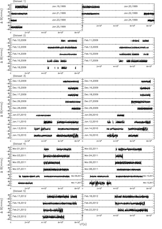
Light curves of all our observations in B for KUV 08368+4026.

Open in new tab Download slide

Table 1.

Open in new tab

Journal of observations for KUV 08368+4026.

Data set	Date	Observatory	Telescope	Frame
1	Jan. 19–25, 1999	Haute-Provence	1.93 m	–
2	Feb. 10–18, 2009	Lijiang	2.4 m	6805
	Dec. 12–18, 2009	Xinglong	2.16 m	1651
	Dec. 26–31, 2009	Lijiang	2.4 m	2328
3	Dec. 27–28, 2009	Xinglong	2.16 m	815
	Jan. 07–17, 2010	SPM	1.5 m	2771
	Jan. 12–19, 2010	Xinglong	2.16 m	2745
	Mar. 01–03, 2011	Xinglong	80 cm	1516
	Mar. 04–07, 2011	Xinglong	85 cm	1746
4	Mar. 08–10, 2011	Xinglong	2.16 m	1655
	Mar. 08–11, 2011	OAGH	2.1 m	1556
5	Feb. 17–23, 2012	Xinglong	2.16 m	3976

Data set	Date	Observatory	Telescope	Frame
1	Jan. 19–25, 1999	Haute-Provence	1.93 m	–
2	Feb. 10–18, 2009	Lijiang	2.4 m	6805
	Dec. 12–18, 2009	Xinglong	2.16 m	1651
	Dec. 26–31, 2009	Lijiang	2.4 m	2328
3	Dec. 27–28, 2009	Xinglong	2.16 m	815
	Jan. 07–17, 2010	SPM	1.5 m	2771
	Jan. 12–19, 2010	Xinglong	2.16 m	2745
	Mar. 01–03, 2011	Xinglong	80 cm	1516
	Mar. 04–07, 2011	Xinglong	85 cm	1746
4	Mar. 08–10, 2011	Xinglong	2.16 m	1655
	Mar. 08–11, 2011	OAGH	2.1 m	1556
5	Feb. 17–23, 2012	Xinglong	2.16 m	3976

Table 1.

Open in new tab

Journal of observations for KUV 08368+4026.

Data set	Date	Observatory	Telescope	Frame
1	Jan. 19–25, 1999	Haute-Provence	1.93 m	–
2	Feb. 10–18, 2009	Lijiang	2.4 m	6805
	Dec. 12–18, 2009	Xinglong	2.16 m	1651
	Dec. 26–31, 2009	Lijiang	2.4 m	2328
3	Dec. 27–28, 2009	Xinglong	2.16 m	815
	Jan. 07–17, 2010	SPM	1.5 m	2771
	Jan. 12–19, 2010	Xinglong	2.16 m	2745
	Mar. 01–03, 2011	Xinglong	80 cm	1516
	Mar. 04–07, 2011	Xinglong	85 cm	1746
4	Mar. 08–10, 2011	Xinglong	2.16 m	1655
	Mar. 08–11, 2011	OAGH	2.1 m	1556
5	Feb. 17–23, 2012	Xinglong	2.16 m	3976

Data set	Date	Observatory	Telescope	Frame
1	Jan. 19–25, 1999	Haute-Provence	1.93 m	–
2	Feb. 10–18, 2009	Lijiang	2.4 m	6805
	Dec. 12–18, 2009	Xinglong	2.16 m	1651
	Dec. 26–31, 2009	Lijiang	2.4 m	2328
3	Dec. 27–28, 2009	Xinglong	2.16 m	815
	Jan. 07–17, 2010	SPM	1.5 m	2771
	Jan. 12–19, 2010	Xinglong	2.16 m	2745
	Mar. 01–03, 2011	Xinglong	80 cm	1516
	Mar. 04–07, 2011	Xinglong	85 cm	1746
4	Mar. 08–10, 2011	Xinglong	2.16 m	1655
	Mar. 08–11, 2011	OAGH	2.1 m	1556
5	Feb. 17–23, 2012	Xinglong	2.16 m	3976

PERIOD ANALYSIS

Period analysis was performed for the light curves by using the software period04 (Lenz & Breger 2005). For all the five data sets, we made Fourier transformation. Fig. 2 shows the Fourier spectra. Note that the amplitudes of the same frequencies vary among the observation runs and this will be discussed in Section 5.

Figure 2.

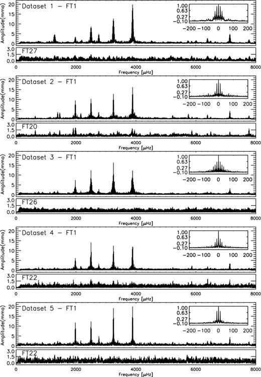
Fourier transformations of the light curves for the five data sets from the top to the bottom. For each data set, the full spectrum before pre-whitening is shown in the upper panel while the spectrum window and the residuals (after removal of the significant frequencies extracted through the pre-whitening process) are shown in the insets and the lower panels, respectively.

Open in new tab Download slide

The data analysis followed the following steps: (1) extract the highest peak from the Fourier spectrum, get its frequency and amplitude and calculate its phase through fitting. (2) Pre-whiten the sine function, make the Fourier transformation for the residuals in order to get the next frequency. We repeated the steps and got finally a list of frequencies with S/N ratio larger than 4. The extracted frequencies are listed in Table 2. Monte Carlo simulations were used to derive the uncertainties on frequencies and amplitudes. We refer to Fu et al. (2013) for more detail about the method based on Monte Carlo simulations.

Table 2.

Open in new tab

Frequency list for the five data sets. f is the frequency in |$\mu \text{Hz}$| and A is the amplitude in mma. The ‘Note’ column indicates the linear combinations, |$ia=11.574\, \mu \text{Hz}$| is the one-day aliasing. The label of the frequencies for each data set follows the order of decreasing amplitude.

(Data set 1)				(Data set 2)				(Data set 3)
ID	f ± 3σ	A±3σ	Note	ID	f ± 3σ	A±3σ	Note	ID	f ± 3σ	A±3σ	Note
a24	747.31 ± 0.22	1.56 ± 0.73	a2–a4	b9	1386.90 ± 0.05	3.63 ± 0.61	b1–b6	c16	747.51 ± 0.08	1.84 ± 0.66	c1–c2
a26	1115.80 ± 0.33	1.55 ± 0.67		b11	1454.67 ± 0.08	3.36 ± 0.59		c22	875.50 ± 0.09	1.42 ± 0.72
a16	1278.72 ± 0.21	2.44 ± 0.80		b4	1976.48 ± 0.03	9.92 ± 0.65		c20	1127.55 ± 0.13	1.53 ± 0.59	c4–c11
a10	1280.51 ± 0.14	4.23 ± 0.78		b13	2159.09 ± 0.07	2.75 ± 0.63		c15	1270.98 ± 0.04	1.85 ± 0.75	c1–c21
a9	1283.64 ± 0.13	5.24 ± 0.77		b3	2498.76 ± 0.02	9.71 ± 0.62		c13	1387.15 ± 0.06	2.27 ± 0.71	c4–c2
a21	1961.68 ± 0.53	1.70 ± 0.82	a14–a9	b6	2500.71 ± 0.02	8.03 ± 0.70		c21	1975.43 ± 0.05	3.07 ± 0.91
a12	1976.10 ± 0.15	3.32 ± 1.05		b19	2757.87 ± 0.08	2.12 ± 0.58		c5	1976.44 ± 0.02	7.64 ± 0.90
a20	2191.49 ± 0.39	1.80 ± 0.94		b10	2759.99 ± 0.05	3.34 ± 0.64		c12	1977.42 ± 0.05	3.16 ± 0.65
a6	2498.85 ± 0.05	7.33 ± 0.87		b16	3245.51 ± 0.11	2.73 ± 0.52		c14	2159.25 ± 0.08	2.21 ± 0.72
a4	2501.15 ± 0.07	7.42 ± 0.71		b2	3246.74 ± 0.03	11.95 ± 0.72		c2	2498.91 ± 0.01	12.60 ± 0.77
a19	2606.27 ± 0.58	1.77 ± 0.99		b8	3247.77 ± 0.06	4.85 ± 0.69		c6	2500.62 ± 0.03	5.90 ± 0.96
a8	2758.81 ± 0.10	5.12 ± 0.79		b17	3249.11 ± 0.11	2.50 ± 0.58	b1+b2–b5	c11	2758.44 ± 0.04	2.74 ± 0.67
a22	2760.75 ± 0.28	1.74 ± 0.80	a18–a3	b5	3885.53 ± 0.02	10.09 ± 0.47		c10	2760.33 ± 0.08	2.97 ± 0.82
a14	3244.98 ± 0.25	3.24 ± 0.90		b12	3886.75 ± 0.04	4.35 ± 0.85		c1	3246.39 ± 0.01	15.41 ± 0.98
a3	3246.43 ± 0.10	9.83 ± 0.83		b1	3887.73 ± 0.02	15.31 ± 0.76		c25	3247.29 ± 0.03	2.40 ± 0.97	c9–c3
a2	3248.13 ± 0.08	12.91 ± 0.73		b18	5223.79 ± 0.07	2.17 ± 0.61	b4+b8	c8	3248.56 ± 0.02	5.39 ± 0.82
a11	3249.32 ± 0.24	4.24 ± 0.93		b14	5747.68 ± 0.07	2.74 ± 0.70	b6+b2	c4	3886.01 ± 0.01	11.12 ± 0.78
a1	3886.25 ± 0.02	20.68 ± 0.77		b15	6386.52 ± 0.06	2.40 ± 0.60	b3+b1	c3	3887.13 ± 0.02	9.76 ± 0.91
a5	3888.25 ± 0.06	7.35 ± 0.62		b7	7134.37 ± 0.05	4.28 ± 0.70	b2+b1	c7	3888.02 ± 0.02	8.28 ± 0.74
a5	3888.25 ± 0.06	7.35 ± 0.62		b7	7134.37 ± 0.05	4.28 ± 0.70	b2+b1	c7	3888.02 ± 0.02	8.28 ± 0.74
a23	4526.86 ± 0.73	1.59 ± 0.77	a16+a2					c23	5747.48 ± 0.09	1.43 ± 0.72	c6+c1
a25	5735.79 ± 0.33	1.54 ± 0.82						c19	5863.48 ± 0.06	1.48 ± 0.61	c12+c4
a18	6007.03 ± 0.24	1.87 ± 0.88	a8+a2					c18	6385.99 ± 0.13	1.64 ± 0.74	c2+c3
a13	6387.46 ± 0.10	3.04 ± 0.64	a4+a1					c24	6492.81 ± 0.09	1.41 ± 0.75
a17	6495.03 ± 0.33	1.93 ± 0.72	a3+a2					c9	7134.27 ± 0.03	3.32 ± 0.69	c1+c7
a7	7134.46 ± 0.08	5.27 ± 0.85	a2+a1					c17	7774.06 ± 0.08	1.66 ± 0.87	c4+c7
a15	7774.32 ± 0.17	2.29 ± 0.81	a1+a5
(Data set 4)				(Data set 5)
ID	f ± 3σ	A±3σ	Note	ID	f ± 3σ	A±3σ	Note
d17	1975.23 ± 0.49	2.68 ± 1.60		e21	872.54 ± 0.25	2.08 ± 1.20
d6	1976.33 ± 0.22	7.87 ± 2.89		e13	1387.16 ± 0.19	2.71 ± 1.47	e1–e3
d9	1977.21 ± 0.35	4.92 ± 3.78		e22	1454.68 ± 0.34	2.05 ± 1.14
d21	2159.12 ± 0.36	2.07 ± 0.92		e15	1911.02 ± 0.68	2.32 ± 1.31	e1–e4
d12	2488.34 ± 0.14	3.46 ± 0.92	d1–ia	e4	1976.51 ± 0.06	12.06 ± 1.34
d1	2498.94 ± 0.06	14.15 ± 0.98		e11	2159.33 ± 0.28	2.69 ± 1.52
d10	2509.96 ± 0.12	4.11 ± 0.86	d1+ia	e5	2498.65 ± 0.09	9.47 ± 1.17
d16	2514.12 ± 0.16	2.67 ± 0.92		e3	2500.66 ± 0.06	10.69 ± 1.45
d18	2748.33 ± 0.35	2.30 ± 0.77	d14–ia	e8	2760.33 ± 0.14	4.79 ± 1.37
d14	2758.30 ± 0.27	3.22 ± 0.83		e2	3246.46 ± 0.04	18.69 ± 1.45
d7	3245.72 ± 0.14	6.21 ± 2.26		e7	3248.44 ± 0.10	6.90 ± 1.32
d2	3246.79 ± 0.22	14.55 ± 1.84		e10	3387.63 ± 0.18	3.18 ± 1.42
d8	3247.96 ± 0.53	5.82 ± 1.80		e6	3885.75 ± 0.09	9.16 ± 1.52
d15	3874.58 ± 0.55	4.94 ± 0.96	d5–ia	e1	3887.78 ± 0.04	18.02 ± 1.40
d11	3885.73 ± 0.19	7.15 ± 5.69		e18	3952.66 ± 0.26	2.22 ± 1.28
d3	3886.81 ± 0.21	17.06 ± 2.28		e20	4477.19 ± 0.20	2.10 ± 1.13	e4+e3
d5	3888.04 ± 0.23	8.64 ± 1.60		e19	5234.48 ± 0.29	2.21 ± 1.08
d4	3897.58 ± 0.27	6.30 ± 1.67	d3+ia	e12	6386.16 ± 0.26	2.61 ± 1.20	e5+e1
d20	5863.43 ± 0.41	2.13 ± 0.78	d6+d3	e14	6494.87 ± 0.20	2.55 ± 1.27	e2+e7
d19	7122.88 ± 0.35	2.64 ± 1.09	d8+d15	e16	7132.20 ± 0.23	2.34 ± 1.17	e2+e6
d13	7145.87 ± 0.53	2.52 ± 0.85	d8+d4	e9	7134.29 ± 0.16	4.26 ± 1.34	e2+e1
				e17	7773.71 ± 0.51	2.23 ± 1.1019	e6+e1

(Data set 1)				(Data set 2)				(Data set 3)
ID	f ± 3σ	A±3σ	Note	ID	f ± 3σ	A±3σ	Note	ID	f ± 3σ	A±3σ	Note
a24	747.31 ± 0.22	1.56 ± 0.73	a2–a4	b9	1386.90 ± 0.05	3.63 ± 0.61	b1–b6	c16	747.51 ± 0.08	1.84 ± 0.66	c1–c2
a26	1115.80 ± 0.33	1.55 ± 0.67		b11	1454.67 ± 0.08	3.36 ± 0.59		c22	875.50 ± 0.09	1.42 ± 0.72
a16	1278.72 ± 0.21	2.44 ± 0.80		b4	1976.48 ± 0.03	9.92 ± 0.65		c20	1127.55 ± 0.13	1.53 ± 0.59	c4–c11
a10	1280.51 ± 0.14	4.23 ± 0.78		b13	2159.09 ± 0.07	2.75 ± 0.63		c15	1270.98 ± 0.04	1.85 ± 0.75	c1–c21
a9	1283.64 ± 0.13	5.24 ± 0.77		b3	2498.76 ± 0.02	9.71 ± 0.62		c13	1387.15 ± 0.06	2.27 ± 0.71	c4–c2
a21	1961.68 ± 0.53	1.70 ± 0.82	a14–a9	b6	2500.71 ± 0.02	8.03 ± 0.70		c21	1975.43 ± 0.05	3.07 ± 0.91
a12	1976.10 ± 0.15	3.32 ± 1.05		b19	2757.87 ± 0.08	2.12 ± 0.58		c5	1976.44 ± 0.02	7.64 ± 0.90
a20	2191.49 ± 0.39	1.80 ± 0.94		b10	2759.99 ± 0.05	3.34 ± 0.64		c12	1977.42 ± 0.05	3.16 ± 0.65
a6	2498.85 ± 0.05	7.33 ± 0.87		b16	3245.51 ± 0.11	2.73 ± 0.52		c14	2159.25 ± 0.08	2.21 ± 0.72
a4	2501.15 ± 0.07	7.42 ± 0.71		b2	3246.74 ± 0.03	11.95 ± 0.72		c2	2498.91 ± 0.01	12.60 ± 0.77
a19	2606.27 ± 0.58	1.77 ± 0.99		b8	3247.77 ± 0.06	4.85 ± 0.69		c6	2500.62 ± 0.03	5.90 ± 0.96
a8	2758.81 ± 0.10	5.12 ± 0.79		b17	3249.11 ± 0.11	2.50 ± 0.58	b1+b2–b5	c11	2758.44 ± 0.04	2.74 ± 0.67
a22	2760.75 ± 0.28	1.74 ± 0.80	a18–a3	b5	3885.53 ± 0.02	10.09 ± 0.47		c10	2760.33 ± 0.08	2.97 ± 0.82
a14	3244.98 ± 0.25	3.24 ± 0.90		b12	3886.75 ± 0.04	4.35 ± 0.85		c1	3246.39 ± 0.01	15.41 ± 0.98
a3	3246.43 ± 0.10	9.83 ± 0.83		b1	3887.73 ± 0.02	15.31 ± 0.76		c25	3247.29 ± 0.03	2.40 ± 0.97	c9–c3
a2	3248.13 ± 0.08	12.91 ± 0.73		b18	5223.79 ± 0.07	2.17 ± 0.61	b4+b8	c8	3248.56 ± 0.02	5.39 ± 0.82
a11	3249.32 ± 0.24	4.24 ± 0.93		b14	5747.68 ± 0.07	2.74 ± 0.70	b6+b2	c4	3886.01 ± 0.01	11.12 ± 0.78
a1	3886.25 ± 0.02	20.68 ± 0.77		b15	6386.52 ± 0.06	2.40 ± 0.60	b3+b1	c3	3887.13 ± 0.02	9.76 ± 0.91
a5	3888.25 ± 0.06	7.35 ± 0.62		b7	7134.37 ± 0.05	4.28 ± 0.70	b2+b1	c7	3888.02 ± 0.02	8.28 ± 0.74
a5	3888.25 ± 0.06	7.35 ± 0.62		b7	7134.37 ± 0.05	4.28 ± 0.70	b2+b1	c7	3888.02 ± 0.02	8.28 ± 0.74
a23	4526.86 ± 0.73	1.59 ± 0.77	a16+a2					c23	5747.48 ± 0.09	1.43 ± 0.72	c6+c1
a25	5735.79 ± 0.33	1.54 ± 0.82						c19	5863.48 ± 0.06	1.48 ± 0.61	c12+c4
a18	6007.03 ± 0.24	1.87 ± 0.88	a8+a2					c18	6385.99 ± 0.13	1.64 ± 0.74	c2+c3
a13	6387.46 ± 0.10	3.04 ± 0.64	a4+a1					c24	6492.81 ± 0.09	1.41 ± 0.75
a17	6495.03 ± 0.33	1.93 ± 0.72	a3+a2					c9	7134.27 ± 0.03	3.32 ± 0.69	c1+c7
a7	7134.46 ± 0.08	5.27 ± 0.85	a2+a1					c17	7774.06 ± 0.08	1.66 ± 0.87	c4+c7
a15	7774.32 ± 0.17	2.29 ± 0.81	a1+a5
(Data set 4)				(Data set 5)
ID	f ± 3σ	A±3σ	Note	ID	f ± 3σ	A±3σ	Note
d17	1975.23 ± 0.49	2.68 ± 1.60		e21	872.54 ± 0.25	2.08 ± 1.20
d6	1976.33 ± 0.22	7.87 ± 2.89		e13	1387.16 ± 0.19	2.71 ± 1.47	e1–e3
d9	1977.21 ± 0.35	4.92 ± 3.78		e22	1454.68 ± 0.34	2.05 ± 1.14
d21	2159.12 ± 0.36	2.07 ± 0.92		e15	1911.02 ± 0.68	2.32 ± 1.31	e1–e4
d12	2488.34 ± 0.14	3.46 ± 0.92	d1–ia	e4	1976.51 ± 0.06	12.06 ± 1.34
d1	2498.94 ± 0.06	14.15 ± 0.98		e11	2159.33 ± 0.28	2.69 ± 1.52
d10	2509.96 ± 0.12	4.11 ± 0.86	d1+ia	e5	2498.65 ± 0.09	9.47 ± 1.17
d16	2514.12 ± 0.16	2.67 ± 0.92		e3	2500.66 ± 0.06	10.69 ± 1.45
d18	2748.33 ± 0.35	2.30 ± 0.77	d14–ia	e8	2760.33 ± 0.14	4.79 ± 1.37
d14	2758.30 ± 0.27	3.22 ± 0.83		e2	3246.46 ± 0.04	18.69 ± 1.45
d7	3245.72 ± 0.14	6.21 ± 2.26		e7	3248.44 ± 0.10	6.90 ± 1.32
d2	3246.79 ± 0.22	14.55 ± 1.84		e10	3387.63 ± 0.18	3.18 ± 1.42
d8	3247.96 ± 0.53	5.82 ± 1.80		e6	3885.75 ± 0.09	9.16 ± 1.52
d15	3874.58 ± 0.55	4.94 ± 0.96	d5–ia	e1	3887.78 ± 0.04	18.02 ± 1.40
d11	3885.73 ± 0.19	7.15 ± 5.69		e18	3952.66 ± 0.26	2.22 ± 1.28
d3	3886.81 ± 0.21	17.06 ± 2.28		e20	4477.19 ± 0.20	2.10 ± 1.13	e4+e3
d5	3888.04 ± 0.23	8.64 ± 1.60		e19	5234.48 ± 0.29	2.21 ± 1.08
d4	3897.58 ± 0.27	6.30 ± 1.67	d3+ia	e12	6386.16 ± 0.26	2.61 ± 1.20	e5+e1
d20	5863.43 ± 0.41	2.13 ± 0.78	d6+d3	e14	6494.87 ± 0.20	2.55 ± 1.27	e2+e7
d19	7122.88 ± 0.35	2.64 ± 1.09	d8+d15	e16	7132.20 ± 0.23	2.34 ± 1.17	e2+e6
d13	7145.87 ± 0.53	2.52 ± 0.85	d8+d4	e9	7134.29 ± 0.16	4.26 ± 1.34	e2+e1
				e17	7773.71 ± 0.51	2.23 ± 1.1019	e6+e1

Table 2.

Open in new tab

Frequency list for the five data sets. f is the frequency in |$\mu \text{Hz}$| and A is the amplitude in mma. The ‘Note’ column indicates the linear combinations, |$ia=11.574\, \mu \text{Hz}$| is the one-day aliasing. The label of the frequencies for each data set follows the order of decreasing amplitude.

(Data set 1)				(Data set 2)				(Data set 3)
ID	f ± 3σ	A±3σ	Note	ID	f ± 3σ	A±3σ	Note	ID	f ± 3σ	A±3σ	Note
a24	747.31 ± 0.22	1.56 ± 0.73	a2–a4	b9	1386.90 ± 0.05	3.63 ± 0.61	b1–b6	c16	747.51 ± 0.08	1.84 ± 0.66	c1–c2
a26	1115.80 ± 0.33	1.55 ± 0.67		b11	1454.67 ± 0.08	3.36 ± 0.59		c22	875.50 ± 0.09	1.42 ± 0.72
a16	1278.72 ± 0.21	2.44 ± 0.80		b4	1976.48 ± 0.03	9.92 ± 0.65		c20	1127.55 ± 0.13	1.53 ± 0.59	c4–c11
a10	1280.51 ± 0.14	4.23 ± 0.78		b13	2159.09 ± 0.07	2.75 ± 0.63		c15	1270.98 ± 0.04	1.85 ± 0.75	c1–c21
a9	1283.64 ± 0.13	5.24 ± 0.77		b3	2498.76 ± 0.02	9.71 ± 0.62		c13	1387.15 ± 0.06	2.27 ± 0.71	c4–c2
a21	1961.68 ± 0.53	1.70 ± 0.82	a14–a9	b6	2500.71 ± 0.02	8.03 ± 0.70		c21	1975.43 ± 0.05	3.07 ± 0.91
a12	1976.10 ± 0.15	3.32 ± 1.05		b19	2757.87 ± 0.08	2.12 ± 0.58		c5	1976.44 ± 0.02	7.64 ± 0.90
a20	2191.49 ± 0.39	1.80 ± 0.94		b10	2759.99 ± 0.05	3.34 ± 0.64		c12	1977.42 ± 0.05	3.16 ± 0.65
a6	2498.85 ± 0.05	7.33 ± 0.87		b16	3245.51 ± 0.11	2.73 ± 0.52		c14	2159.25 ± 0.08	2.21 ± 0.72
a4	2501.15 ± 0.07	7.42 ± 0.71		b2	3246.74 ± 0.03	11.95 ± 0.72		c2	2498.91 ± 0.01	12.60 ± 0.77
a19	2606.27 ± 0.58	1.77 ± 0.99		b8	3247.77 ± 0.06	4.85 ± 0.69		c6	2500.62 ± 0.03	5.90 ± 0.96
a8	2758.81 ± 0.10	5.12 ± 0.79		b17	3249.11 ± 0.11	2.50 ± 0.58	b1+b2–b5	c11	2758.44 ± 0.04	2.74 ± 0.67
a22	2760.75 ± 0.28	1.74 ± 0.80	a18–a3	b5	3885.53 ± 0.02	10.09 ± 0.47		c10	2760.33 ± 0.08	2.97 ± 0.82
a14	3244.98 ± 0.25	3.24 ± 0.90		b12	3886.75 ± 0.04	4.35 ± 0.85		c1	3246.39 ± 0.01	15.41 ± 0.98
a3	3246.43 ± 0.10	9.83 ± 0.83		b1	3887.73 ± 0.02	15.31 ± 0.76		c25	3247.29 ± 0.03	2.40 ± 0.97	c9–c3
a2	3248.13 ± 0.08	12.91 ± 0.73		b18	5223.79 ± 0.07	2.17 ± 0.61	b4+b8	c8	3248.56 ± 0.02	5.39 ± 0.82
a11	3249.32 ± 0.24	4.24 ± 0.93		b14	5747.68 ± 0.07	2.74 ± 0.70	b6+b2	c4	3886.01 ± 0.01	11.12 ± 0.78
a1	3886.25 ± 0.02	20.68 ± 0.77		b15	6386.52 ± 0.06	2.40 ± 0.60	b3+b1	c3	3887.13 ± 0.02	9.76 ± 0.91
a5	3888.25 ± 0.06	7.35 ± 0.62		b7	7134.37 ± 0.05	4.28 ± 0.70	b2+b1	c7	3888.02 ± 0.02	8.28 ± 0.74
a5	3888.25 ± 0.06	7.35 ± 0.62		b7	7134.37 ± 0.05	4.28 ± 0.70	b2+b1	c7	3888.02 ± 0.02	8.28 ± 0.74
a23	4526.86 ± 0.73	1.59 ± 0.77	a16+a2					c23	5747.48 ± 0.09	1.43 ± 0.72	c6+c1
a25	5735.79 ± 0.33	1.54 ± 0.82						c19	5863.48 ± 0.06	1.48 ± 0.61	c12+c4
a18	6007.03 ± 0.24	1.87 ± 0.88	a8+a2					c18	6385.99 ± 0.13	1.64 ± 0.74	c2+c3
a13	6387.46 ± 0.10	3.04 ± 0.64	a4+a1					c24	6492.81 ± 0.09	1.41 ± 0.75
a17	6495.03 ± 0.33	1.93 ± 0.72	a3+a2					c9	7134.27 ± 0.03	3.32 ± 0.69	c1+c7
a7	7134.46 ± 0.08	5.27 ± 0.85	a2+a1					c17	7774.06 ± 0.08	1.66 ± 0.87	c4+c7
a15	7774.32 ± 0.17	2.29 ± 0.81	a1+a5
(Data set 4)				(Data set 5)
ID	f ± 3σ	A±3σ	Note	ID	f ± 3σ	A±3σ	Note
d17	1975.23 ± 0.49	2.68 ± 1.60		e21	872.54 ± 0.25	2.08 ± 1.20
d6	1976.33 ± 0.22	7.87 ± 2.89		e13	1387.16 ± 0.19	2.71 ± 1.47	e1–e3
d9	1977.21 ± 0.35	4.92 ± 3.78		e22	1454.68 ± 0.34	2.05 ± 1.14
d21	2159.12 ± 0.36	2.07 ± 0.92		e15	1911.02 ± 0.68	2.32 ± 1.31	e1–e4
d12	2488.34 ± 0.14	3.46 ± 0.92	d1–ia	e4	1976.51 ± 0.06	12.06 ± 1.34
d1	2498.94 ± 0.06	14.15 ± 0.98		e11	2159.33 ± 0.28	2.69 ± 1.52
d10	2509.96 ± 0.12	4.11 ± 0.86	d1+ia	e5	2498.65 ± 0.09	9.47 ± 1.17
d16	2514.12 ± 0.16	2.67 ± 0.92		e3	2500.66 ± 0.06	10.69 ± 1.45
d18	2748.33 ± 0.35	2.30 ± 0.77	d14–ia	e8	2760.33 ± 0.14	4.79 ± 1.37
d14	2758.30 ± 0.27	3.22 ± 0.83		e2	3246.46 ± 0.04	18.69 ± 1.45
d7	3245.72 ± 0.14	6.21 ± 2.26		e7	3248.44 ± 0.10	6.90 ± 1.32
d2	3246.79 ± 0.22	14.55 ± 1.84		e10	3387.63 ± 0.18	3.18 ± 1.42
d8	3247.96 ± 0.53	5.82 ± 1.80		e6	3885.75 ± 0.09	9.16 ± 1.52
d15	3874.58 ± 0.55	4.94 ± 0.96	d5–ia	e1	3887.78 ± 0.04	18.02 ± 1.40
d11	3885.73 ± 0.19	7.15 ± 5.69		e18	3952.66 ± 0.26	2.22 ± 1.28
d3	3886.81 ± 0.21	17.06 ± 2.28		e20	4477.19 ± 0.20	2.10 ± 1.13	e4+e3
d5	3888.04 ± 0.23	8.64 ± 1.60		e19	5234.48 ± 0.29	2.21 ± 1.08
d4	3897.58 ± 0.27	6.30 ± 1.67	d3+ia	e12	6386.16 ± 0.26	2.61 ± 1.20	e5+e1
d20	5863.43 ± 0.41	2.13 ± 0.78	d6+d3	e14	6494.87 ± 0.20	2.55 ± 1.27	e2+e7
d19	7122.88 ± 0.35	2.64 ± 1.09	d8+d15	e16	7132.20 ± 0.23	2.34 ± 1.17	e2+e6
d13	7145.87 ± 0.53	2.52 ± 0.85	d8+d4	e9	7134.29 ± 0.16	4.26 ± 1.34	e2+e1
				e17	7773.71 ± 0.51	2.23 ± 1.1019	e6+e1

(Data set 1)				(Data set 2)				(Data set 3)
ID	f ± 3σ	A±3σ	Note	ID	f ± 3σ	A±3σ	Note	ID	f ± 3σ	A±3σ	Note
a24	747.31 ± 0.22	1.56 ± 0.73	a2–a4	b9	1386.90 ± 0.05	3.63 ± 0.61	b1–b6	c16	747.51 ± 0.08	1.84 ± 0.66	c1–c2
a26	1115.80 ± 0.33	1.55 ± 0.67		b11	1454.67 ± 0.08	3.36 ± 0.59		c22	875.50 ± 0.09	1.42 ± 0.72
a16	1278.72 ± 0.21	2.44 ± 0.80		b4	1976.48 ± 0.03	9.92 ± 0.65		c20	1127.55 ± 0.13	1.53 ± 0.59	c4–c11
a10	1280.51 ± 0.14	4.23 ± 0.78		b13	2159.09 ± 0.07	2.75 ± 0.63		c15	1270.98 ± 0.04	1.85 ± 0.75	c1–c21
a9	1283.64 ± 0.13	5.24 ± 0.77		b3	2498.76 ± 0.02	9.71 ± 0.62		c13	1387.15 ± 0.06	2.27 ± 0.71	c4–c2
a21	1961.68 ± 0.53	1.70 ± 0.82	a14–a9	b6	2500.71 ± 0.02	8.03 ± 0.70		c21	1975.43 ± 0.05	3.07 ± 0.91
a12	1976.10 ± 0.15	3.32 ± 1.05		b19	2757.87 ± 0.08	2.12 ± 0.58		c5	1976.44 ± 0.02	7.64 ± 0.90
a20	2191.49 ± 0.39	1.80 ± 0.94		b10	2759.99 ± 0.05	3.34 ± 0.64		c12	1977.42 ± 0.05	3.16 ± 0.65
a6	2498.85 ± 0.05	7.33 ± 0.87		b16	3245.51 ± 0.11	2.73 ± 0.52		c14	2159.25 ± 0.08	2.21 ± 0.72
a4	2501.15 ± 0.07	7.42 ± 0.71		b2	3246.74 ± 0.03	11.95 ± 0.72		c2	2498.91 ± 0.01	12.60 ± 0.77
a19	2606.27 ± 0.58	1.77 ± 0.99		b8	3247.77 ± 0.06	4.85 ± 0.69		c6	2500.62 ± 0.03	5.90 ± 0.96
a8	2758.81 ± 0.10	5.12 ± 0.79		b17	3249.11 ± 0.11	2.50 ± 0.58	b1+b2–b5	c11	2758.44 ± 0.04	2.74 ± 0.67
a22	2760.75 ± 0.28	1.74 ± 0.80	a18–a3	b5	3885.53 ± 0.02	10.09 ± 0.47		c10	2760.33 ± 0.08	2.97 ± 0.82
a14	3244.98 ± 0.25	3.24 ± 0.90		b12	3886.75 ± 0.04	4.35 ± 0.85		c1	3246.39 ± 0.01	15.41 ± 0.98
a3	3246.43 ± 0.10	9.83 ± 0.83		b1	3887.73 ± 0.02	15.31 ± 0.76		c25	3247.29 ± 0.03	2.40 ± 0.97	c9–c3
a2	3248.13 ± 0.08	12.91 ± 0.73		b18	5223.79 ± 0.07	2.17 ± 0.61	b4+b8	c8	3248.56 ± 0.02	5.39 ± 0.82
a11	3249.32 ± 0.24	4.24 ± 0.93		b14	5747.68 ± 0.07	2.74 ± 0.70	b6+b2	c4	3886.01 ± 0.01	11.12 ± 0.78
a1	3886.25 ± 0.02	20.68 ± 0.77		b15	6386.52 ± 0.06	2.40 ± 0.60	b3+b1	c3	3887.13 ± 0.02	9.76 ± 0.91
a5	3888.25 ± 0.06	7.35 ± 0.62		b7	7134.37 ± 0.05	4.28 ± 0.70	b2+b1	c7	3888.02 ± 0.02	8.28 ± 0.74
a5	3888.25 ± 0.06	7.35 ± 0.62		b7	7134.37 ± 0.05	4.28 ± 0.70	b2+b1	c7	3888.02 ± 0.02	8.28 ± 0.74
a23	4526.86 ± 0.73	1.59 ± 0.77	a16+a2					c23	5747.48 ± 0.09	1.43 ± 0.72	c6+c1
a25	5735.79 ± 0.33	1.54 ± 0.82						c19	5863.48 ± 0.06	1.48 ± 0.61	c12+c4
a18	6007.03 ± 0.24	1.87 ± 0.88	a8+a2					c18	6385.99 ± 0.13	1.64 ± 0.74	c2+c3
a13	6387.46 ± 0.10	3.04 ± 0.64	a4+a1					c24	6492.81 ± 0.09	1.41 ± 0.75
a17	6495.03 ± 0.33	1.93 ± 0.72	a3+a2					c9	7134.27 ± 0.03	3.32 ± 0.69	c1+c7
a7	7134.46 ± 0.08	5.27 ± 0.85	a2+a1					c17	7774.06 ± 0.08	1.66 ± 0.87	c4+c7
a15	7774.32 ± 0.17	2.29 ± 0.81	a1+a5
(Data set 4)				(Data set 5)
ID	f ± 3σ	A±3σ	Note	ID	f ± 3σ	A±3σ	Note
d17	1975.23 ± 0.49	2.68 ± 1.60		e21	872.54 ± 0.25	2.08 ± 1.20
d6	1976.33 ± 0.22	7.87 ± 2.89		e13	1387.16 ± 0.19	2.71 ± 1.47	e1–e3
d9	1977.21 ± 0.35	4.92 ± 3.78		e22	1454.68 ± 0.34	2.05 ± 1.14
d21	2159.12 ± 0.36	2.07 ± 0.92		e15	1911.02 ± 0.68	2.32 ± 1.31	e1–e4
d12	2488.34 ± 0.14	3.46 ± 0.92	d1–ia	e4	1976.51 ± 0.06	12.06 ± 1.34
d1	2498.94 ± 0.06	14.15 ± 0.98		e11	2159.33 ± 0.28	2.69 ± 1.52
d10	2509.96 ± 0.12	4.11 ± 0.86	d1+ia	e5	2498.65 ± 0.09	9.47 ± 1.17
d16	2514.12 ± 0.16	2.67 ± 0.92		e3	2500.66 ± 0.06	10.69 ± 1.45
d18	2748.33 ± 0.35	2.30 ± 0.77	d14–ia	e8	2760.33 ± 0.14	4.79 ± 1.37
d14	2758.30 ± 0.27	3.22 ± 0.83		e2	3246.46 ± 0.04	18.69 ± 1.45
d7	3245.72 ± 0.14	6.21 ± 2.26		e7	3248.44 ± 0.10	6.90 ± 1.32
d2	3246.79 ± 0.22	14.55 ± 1.84		e10	3387.63 ± 0.18	3.18 ± 1.42
d8	3247.96 ± 0.53	5.82 ± 1.80		e6	3885.75 ± 0.09	9.16 ± 1.52
d15	3874.58 ± 0.55	4.94 ± 0.96	d5–ia	e1	3887.78 ± 0.04	18.02 ± 1.40
d11	3885.73 ± 0.19	7.15 ± 5.69		e18	3952.66 ± 0.26	2.22 ± 1.28
d3	3886.81 ± 0.21	17.06 ± 2.28		e20	4477.19 ± 0.20	2.10 ± 1.13	e4+e3
d5	3888.04 ± 0.23	8.64 ± 1.60		e19	5234.48 ± 0.29	2.21 ± 1.08
d4	3897.58 ± 0.27	6.30 ± 1.67	d3+ia	e12	6386.16 ± 0.26	2.61 ± 1.20	e5+e1
d20	5863.43 ± 0.41	2.13 ± 0.78	d6+d3	e14	6494.87 ± 0.20	2.55 ± 1.27	e2+e7
d19	7122.88 ± 0.35	2.64 ± 1.09	d8+d15	e16	7132.20 ± 0.23	2.34 ± 1.17	e2+e6
d13	7145.87 ± 0.53	2.52 ± 0.85	d8+d4	e9	7134.29 ± 0.16	4.26 ± 1.34	e2+e1
				e17	7773.71 ± 0.51	2.23 ± 1.1019	e6+e1

For data set 3, we found a number of extremely-close frequencies with low amplitudes in addition to the major frequencies during the pre-whitening process. After checking the data carefully we realized that it is due to the variation of the amplitudes of the same frequencies on the time-scale of weeks, thus the pre-whitening of the frequency could not be completely done with a fixed amplitude and phase. The subroutine ‘Calculate amplitude/phase variations’ of Period04 was then used to solve this problem. For each frequency, individual amplitude and phase were used to pre-whiten the light curves of individual run. The residuals were then combined to calculate the next Fourier transformation.

We compare frequency list of the five data sets in Table 2 to each other in order to identify the same frequencies from different data sets. The result is presented in Table 3.

Table 3.

Open in new tab

Comparison of the frequencies and amplitudes in the five data sets. Note that f = frequency in μHz, A = amplitude in mma.

	(Data set 1)		(Data set 2)		(Data set 3)		(Data set 4)		(Data set 5)
ID	f	A	f	A	f	A	f	A	f	A
F1									872.54	2.08
F2					875.50	1.42
F3	1115.80	1.55
F4	1278.72	2.44
F5	1280.51	4.23
F6	1283.64	5.24
F7			1454.67	3.36					1454.68	2.05
F8					1975.43	3.07	1975.23	2.68
F9	1976.10	3.32	1976.48	9.92	1976.44	7.64	1976.33	7.87	1976.51	12.06
F10					1977.42	3.16	1977.21	4.92
F11			2159.09	2.75	2159.25	2.21	2159.12	2.07	2159.33	2.69
F12	2191.49	1.80
F13	2498.85	7.33	2498.76	9.71	2498.91	12.60	2498.94	14.15	2498.65	9.47
F14	2501.15	7.42	2500.71	8.03	2500.62	5.90			2500.66	10.69
F15							2514.12	2.67
F16	2606.27	1.77
F17	2758.81	5.12	2757.87	2.12	2758.44	2.74	2758.30	3.22
F18			2759.99	3.34	2760.33	2.97			2760.33	4.79
F19	3244.98	3.24	3245.51	2.73			3245.72	6.21
F20	3246.43	9.83	3246.74	11.95	3246.39	15.41	3246.79	14.55	3246.46	18.69
F21	3248.13	12.91	3247.77	4.85	3248.56	5.39	3247.96	5.82	3248.44	6.90
F22	3249.32	4.24
F23									3387.63	3.18
F24	3886.25	20.68	3885.53	10.09	3886.01	11.12	3885.73	7.15	3885.75	9.16
F25			3886.75	4.35	3887.13	9.76	3886.81	17.06
F26	3888.25	7.35	3887.73	15.31	3888.02	8.28	3888.04	8.64	3887.78	18.02
F27									3952.66	2.22
F28									5234.48	2.21
F29	5735.79	1.54
F30					6492.81	1.41

	(Data set 1)		(Data set 2)		(Data set 3)		(Data set 4)		(Data set 5)
ID	f	A	f	A	f	A	f	A	f	A
F1									872.54	2.08
F2					875.50	1.42
F3	1115.80	1.55
F4	1278.72	2.44
F5	1280.51	4.23
F6	1283.64	5.24
F7			1454.67	3.36					1454.68	2.05
F8					1975.43	3.07	1975.23	2.68
F9	1976.10	3.32	1976.48	9.92	1976.44	7.64	1976.33	7.87	1976.51	12.06
F10					1977.42	3.16	1977.21	4.92
F11			2159.09	2.75	2159.25	2.21	2159.12	2.07	2159.33	2.69
F12	2191.49	1.80
F13	2498.85	7.33	2498.76	9.71	2498.91	12.60	2498.94	14.15	2498.65	9.47
F14	2501.15	7.42	2500.71	8.03	2500.62	5.90			2500.66	10.69
F15							2514.12	2.67
F16	2606.27	1.77
F17	2758.81	5.12	2757.87	2.12	2758.44	2.74	2758.30	3.22
F18			2759.99	3.34	2760.33	2.97			2760.33	4.79
F19	3244.98	3.24	3245.51	2.73			3245.72	6.21
F20	3246.43	9.83	3246.74	11.95	3246.39	15.41	3246.79	14.55	3246.46	18.69
F21	3248.13	12.91	3247.77	4.85	3248.56	5.39	3247.96	5.82	3248.44	6.90
F22	3249.32	4.24
F23									3387.63	3.18
F24	3886.25	20.68	3885.53	10.09	3886.01	11.12	3885.73	7.15	3885.75	9.16
F25			3886.75	4.35	3887.13	9.76	3886.81	17.06
F26	3888.25	7.35	3887.73	15.31	3888.02	8.28	3888.04	8.64	3887.78	18.02
F27									3952.66	2.22
F28									5234.48	2.21
F29	5735.79	1.54
F30					6492.81	1.41

Table 3.

Open in new tab

Comparison of the frequencies and amplitudes in the five data sets. Note that f = frequency in μHz, A = amplitude in mma.

	(Data set 1)		(Data set 2)		(Data set 3)		(Data set 4)		(Data set 5)
ID	f	A	f	A	f	A	f	A	f	A
F1									872.54	2.08
F2					875.50	1.42
F3	1115.80	1.55
F4	1278.72	2.44
F5	1280.51	4.23
F6	1283.64	5.24
F7			1454.67	3.36					1454.68	2.05
F8					1975.43	3.07	1975.23	2.68
F9	1976.10	3.32	1976.48	9.92	1976.44	7.64	1976.33	7.87	1976.51	12.06
F10					1977.42	3.16	1977.21	4.92
F11			2159.09	2.75	2159.25	2.21	2159.12	2.07	2159.33	2.69
F12	2191.49	1.80
F13	2498.85	7.33	2498.76	9.71	2498.91	12.60	2498.94	14.15	2498.65	9.47
F14	2501.15	7.42	2500.71	8.03	2500.62	5.90			2500.66	10.69
F15							2514.12	2.67
F16	2606.27	1.77
F17	2758.81	5.12	2757.87	2.12	2758.44	2.74	2758.30	3.22
F18			2759.99	3.34	2760.33	2.97			2760.33	4.79
F19	3244.98	3.24	3245.51	2.73			3245.72	6.21
F20	3246.43	9.83	3246.74	11.95	3246.39	15.41	3246.79	14.55	3246.46	18.69
F21	3248.13	12.91	3247.77	4.85	3248.56	5.39	3247.96	5.82	3248.44	6.90
F22	3249.32	4.24
F23									3387.63	3.18
F24	3886.25	20.68	3885.53	10.09	3886.01	11.12	3885.73	7.15	3885.75	9.16
F25			3886.75	4.35	3887.13	9.76	3886.81	17.06
F26	3888.25	7.35	3887.73	15.31	3888.02	8.28	3888.04	8.64	3887.78	18.02
F27									3952.66	2.22
F28									5234.48	2.21
F29	5735.79	1.54
F30					6492.81	1.41

	(Data set 1)		(Data set 2)		(Data set 3)		(Data set 4)		(Data set 5)
ID	f	A	f	A	f	A	f	A	f	A
F1									872.54	2.08
F2					875.50	1.42
F3	1115.80	1.55
F4	1278.72	2.44
F5	1280.51	4.23
F6	1283.64	5.24
F7			1454.67	3.36					1454.68	2.05
F8					1975.43	3.07	1975.23	2.68
F9	1976.10	3.32	1976.48	9.92	1976.44	7.64	1976.33	7.87	1976.51	12.06
F10					1977.42	3.16	1977.21	4.92
F11			2159.09	2.75	2159.25	2.21	2159.12	2.07	2159.33	2.69
F12	2191.49	1.80
F13	2498.85	7.33	2498.76	9.71	2498.91	12.60	2498.94	14.15	2498.65	9.47
F14	2501.15	7.42	2500.71	8.03	2500.62	5.90			2500.66	10.69
F15							2514.12	2.67
F16	2606.27	1.77
F17	2758.81	5.12	2757.87	2.12	2758.44	2.74	2758.30	3.22
F18			2759.99	3.34	2760.33	2.97			2760.33	4.79
F19	3244.98	3.24	3245.51	2.73			3245.72	6.21
F20	3246.43	9.83	3246.74	11.95	3246.39	15.41	3246.79	14.55	3246.46	18.69
F21	3248.13	12.91	3247.77	4.85	3248.56	5.39	3247.96	5.82	3248.44	6.90
F22	3249.32	4.24
F23									3387.63	3.18
F24	3886.25	20.68	3885.53	10.09	3886.01	11.12	3885.73	7.15	3885.75	9.16
F25			3886.75	4.35	3887.13	9.76	3886.81	17.06
F26	3888.25	7.35	3887.73	15.31	3888.02	8.28	3888.04	8.64	3887.78	18.02
F27									3952.66	2.22
F28									5234.48	2.21
F29	5735.79	1.54
F30					6492.81	1.41

ASTEROSEISMOLOGY

Linear combinations

Since most of runs are single-site observations, aliasing effect is strongly visible in some spectrum windows in Fig. 2, especially in the window spectra of 1999 January of (data set 1), 2009 February (data set 2) and 2012 February (data set 5).

The analysis of linear combinations and aliasing frequencies were made and the result is listed in the column ‘Note’ of Table 2.

Mode identification

After removing the frequencies of linear combination and aliasing, we list the frequencies with amplitudes in Table 3. The frequencies which are components of multiplets, or present large amplitudes, or are detected in multiple seasons are identified as independent signals. For the single frequencies with low amplitudes or detected in only one observing season, we group them as further signals. Please note the frequency of 3249.32 μHz. Although it is close to a triplet, we assign it as a further signal since it is detected only once in a single-site observing run with a photoelectric photometer and its amplitude is small. We summarize the independent frequencies and further signals in Table 4. For the frequencies detected in multiple seasons, we take the average values of the frequencies.

Table 4.

Open in new tab

Signals identified. f = frequency in μHz. A = amplitude in mma. P = Period in seconds.

ID	f	A	P
Independent signals
f1	1278.72	2.44	782.0
f2	1280.51	4.23	780.9
f3	1283.64	5.24	779.0
f4	1975.33	2.88	506.2
f5	1976.37	8.16	506.0
f6	1977.31	4.04	505.7
f7	2159.20	2.43	463.1
f8	2498.82	10.65	400.2
f9	2500.79	8.01	399.9
f10	2758.35	3.30	362.5
f11	2760.22	3.70	362.3
f12	3245.61	4.47	308.1
f13	3246.56	14.09	308.0
f14	3248.17	7.17	307.9
f15	3885.85	11.64	257.3
f16	3886.90	10.39	257.3
f17	3887.96	11.52	257.2
Further signals
f18	872.54	2.08	1146.1
f19	875.50	1.42	1142.2
f20	1115.80	1.55	896.2
f21	1454.68	2.70	687.4
f22	2191.49	1.80	456.3
f23	2514.12	2.67	397.8
f24	2606.27	1.77	383.7
f25	3249.32	4.24	307.8
f26	3387.63	3.18	295.2
f27	3952.66	2.22	253.0
f28	5234.48	2.21	191.0
f29	5735.79	1.54	174.3
f30	6492.81	1.41	154.0

ID	f	A	P
Independent signals
f1	1278.72	2.44	782.0
f2	1280.51	4.23	780.9
f3	1283.64	5.24	779.0
f4	1975.33	2.88	506.2
f5	1976.37	8.16	506.0
f6	1977.31	4.04	505.7
f7	2159.20	2.43	463.1
f8	2498.82	10.65	400.2
f9	2500.79	8.01	399.9
f10	2758.35	3.30	362.5
f11	2760.22	3.70	362.3
f12	3245.61	4.47	308.1
f13	3246.56	14.09	308.0
f14	3248.17	7.17	307.9
f15	3885.85	11.64	257.3
f16	3886.90	10.39	257.3
f17	3887.96	11.52	257.2
Further signals
f18	872.54	2.08	1146.1
f19	875.50	1.42	1142.2
f20	1115.80	1.55	896.2
f21	1454.68	2.70	687.4
f22	2191.49	1.80	456.3
f23	2514.12	2.67	397.8
f24	2606.27	1.77	383.7
f25	3249.32	4.24	307.8
f26	3387.63	3.18	295.2
f27	3952.66	2.22	253.0
f28	5234.48	2.21	191.0
f29	5735.79	1.54	174.3
f30	6492.81	1.41	154.0

Table 4.

Open in new tab

Signals identified. f = frequency in μHz. A = amplitude in mma. P = Period in seconds.

ID	f	A	P
Independent signals
f1	1278.72	2.44	782.0
f2	1280.51	4.23	780.9
f3	1283.64	5.24	779.0
f4	1975.33	2.88	506.2
f5	1976.37	8.16	506.0
f6	1977.31	4.04	505.7
f7	2159.20	2.43	463.1
f8	2498.82	10.65	400.2
f9	2500.79	8.01	399.9
f10	2758.35	3.30	362.5
f11	2760.22	3.70	362.3
f12	3245.61	4.47	308.1
f13	3246.56	14.09	308.0
f14	3248.17	7.17	307.9
f15	3885.85	11.64	257.3
f16	3886.90	10.39	257.3
f17	3887.96	11.52	257.2
Further signals
f18	872.54	2.08	1146.1
f19	875.50	1.42	1142.2
f20	1115.80	1.55	896.2
f21	1454.68	2.70	687.4
f22	2191.49	1.80	456.3
f23	2514.12	2.67	397.8
f24	2606.27	1.77	383.7
f25	3249.32	4.24	307.8
f26	3387.63	3.18	295.2
f27	3952.66	2.22	253.0
f28	5234.48	2.21	191.0
f29	5735.79	1.54	174.3
f30	6492.81	1.41	154.0

ID	f	A	P
Independent signals
f1	1278.72	2.44	782.0
f2	1280.51	4.23	780.9
f3	1283.64	5.24	779.0
f4	1975.33	2.88	506.2
f5	1976.37	8.16	506.0
f6	1977.31	4.04	505.7
f7	2159.20	2.43	463.1
f8	2498.82	10.65	400.2
f9	2500.79	8.01	399.9
f10	2758.35	3.30	362.5
f11	2760.22	3.70	362.3
f12	3245.61	4.47	308.1
f13	3246.56	14.09	308.0
f14	3248.17	7.17	307.9
f15	3885.85	11.64	257.3
f16	3886.90	10.39	257.3
f17	3887.96	11.52	257.2
Further signals
f18	872.54	2.08	1146.1
f19	875.50	1.42	1142.2
f20	1115.80	1.55	896.2
f21	1454.68	2.70	687.4
f22	2191.49	1.80	456.3
f23	2514.12	2.67	397.8
f24	2606.27	1.77	383.7
f25	3249.32	4.24	307.8
f26	3387.63	3.18	295.2
f27	3952.66	2.22	253.0
f28	5234.48	2.21	191.0
f29	5735.79	1.54	174.3
f30	6492.81	1.41	154.0

Four triplets are identified from the independent signals in Table 4. f1–f3 is an unequal triplet. Since the spacing of f3 to f2 is almost twice of the spacing of f1 to f2, we suppose they are l = 2 modes. The other three triplets show nearly equal spacing of about 1 μHz inside the triplets, which is the property of l = 1 modes. We also notice that the two doublets have frequency spacing of about 2 μHz. Thus we identify them as l = 1 modes with the central frequencies of m = 0 mode undetected.

From the equation:

\begin{equation*} \sigma _{k,l,m}=\sigma _{k,l}+m\times (1-C_{k,l}) \Omega , \end{equation*}

where σ_{k, l, m} and σ_{k, l} are the frequencies of the rotating star and non-rotating star of the mode with certain k and l value. C_{k, l} = 1/l(l + 1) in the asymptotic regime (Brickhill 1975). From this equation, one may derive that the splits of the l = 2 modes are 1.67 times of the splits of the l = 1 modes. As far as the triplet around 1280.51 μHz is concerned, the two splits are about 1.6 and 3.2 μHz, which agrees with the early identification of this frequency as an l = 2 mode.

The frequency at 2159.20 μHz will be discussed in Section 4.4 alone.

Rotational splitting

From the five multiplets of the l = 1 modes, we derived an average rotation splitting of 1.049 ± 0.041 μHz. Thus, we estimate the rotation period of KUV 08368+4026 as 5.52 ± 0.22 d.

Period spacing

In Table 3, there are some frequencies which belong to neither doublets nor triplets with amplitudes close to the detection limit and appearing only once among the five observation seasons. We identify these frequencies as further signals in Table 4, except the one at 2159.20 μHz, which has been detected in four seasons hence listed as an independent signal.

Table 5 lists the identified l = 1 frequencies and l = 2 modes in Table a and b, respectively. With the three l = 1 and m = 0 modes in the triplets, we made a linear fit of the periods for the three modes which give an average spacing of 49.2 s. Fig. 3 shows the fitting. We also plot the missing m = 0 modes with the frequency values of the centre of the frequency values of the m = ±1 modes. The single mode at 2159.20 μHz is plotted on the figure as well.

Figure 3.

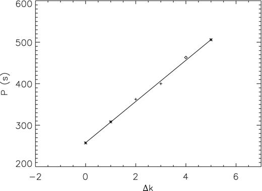
Linear fitting of three l = 1, m = 0 modes (star marks). The crosses show the two doublets, The circle shows the single mode at 2159.60 μHz.

Open in new tab Download slide

Table 5.

Open in new tab

Modes identification for all l = 1 modes(table a) and l = 2 modes(table b). f is the frequencies in μHz, δf is the frequency separation in μHz. P is the period in second and DP is the residual between observing period and the linear fit of period of the five l = 1 modes. For the two doublets, the frequency values of the undetected m = 0 mode are estimated at the centre of the frequency values of the m = ±1 modes.

Table a
f	δf	P	δk	m	DP
1975.33		506.2		−1
	1.04
1976.37		506.0	+ 5	0	1.38
	0.94
1977.31		505.7		+1
2159.20		463.1	+4	0?	7.77
2498.82		400.2		−1
	0.99
2499.81		400.0	+ 3	0	−6.10
	0.98
2500.79		399.9		+1
2758.35		362.5		−1
	0.94
2759.29		362.4	+ 2	0	5.52
	0.93
2760.22		362.3		+1
3245.61		308.1		−1
	0.95
3246.56		308.0	+ 1	0	0.36
	1.61
3248.17		307.9		+1
3885.85		257.3		−1
	1.05
3886.90		257.3	+ 0	0	−1.15
	1.06
3887.96		257.2		+1
Table b
f	δf	P	m
1278.72		782.0	−1
	1.79
1280.51		780.9	0
	3.13
1283.64		779.0	+2

Table a
f	δf	P	δk	m	DP
1975.33		506.2		−1
	1.04
1976.37		506.0	+ 5	0	1.38
	0.94
1977.31		505.7		+1
2159.20		463.1	+4	0?	7.77
2498.82		400.2		−1
	0.99
2499.81		400.0	+ 3	0	−6.10
	0.98
2500.79		399.9		+1
2758.35		362.5		−1
	0.94
2759.29		362.4	+ 2	0	5.52
	0.93
2760.22		362.3		+1
3245.61		308.1		−1
	0.95
3246.56		308.0	+ 1	0	0.36
	1.61
3248.17		307.9		+1
3885.85		257.3		−1
	1.05
3886.90		257.3	+ 0	0	−1.15
	1.06
3887.96		257.2		+1
Table b
f	δf	P	m
1278.72		782.0	−1
	1.79
1280.51		780.9	0
	3.13
1283.64		779.0	+2

Table 5.

Open in new tab

Modes identification for all l = 1 modes(table a) and l = 2 modes(table b). f is the frequencies in μHz, δf is the frequency separation in μHz. P is the period in second and DP is the residual between observing period and the linear fit of period of the five l = 1 modes. For the two doublets, the frequency values of the undetected m = 0 mode are estimated at the centre of the frequency values of the m = ±1 modes.

Table a
f	δf	P	δk	m	DP
1975.33		506.2		−1
	1.04
1976.37		506.0	+ 5	0	1.38
	0.94
1977.31		505.7		+1
2159.20		463.1	+4	0?	7.77
2498.82		400.2		−1
	0.99
2499.81		400.0	+ 3	0	−6.10
	0.98
2500.79		399.9		+1
2758.35		362.5		−1
	0.94
2759.29		362.4	+ 2	0	5.52
	0.93
2760.22		362.3		+1
3245.61		308.1		−1
	0.95
3246.56		308.0	+ 1	0	0.36
	1.61
3248.17		307.9		+1
3885.85		257.3		−1
	1.05
3886.90		257.3	+ 0	0	−1.15
	1.06
3887.96		257.2		+1
Table b
f	δf	P	m
1278.72		782.0	−1
	1.79
1280.51		780.9	0
	3.13
1283.64		779.0	+2

Table a
f	δf	P	δk	m	DP
1975.33		506.2		−1
	1.04
1976.37		506.0	+ 5	0	1.38
	0.94
1977.31		505.7		+1
2159.20		463.1	+4	0?	7.77
2498.82		400.2		−1
	0.99
2499.81		400.0	+ 3	0	−6.10
	0.98
2500.79		399.9		+1
2758.35		362.5		−1
	0.94
2759.29		362.4	+ 2	0	5.52
	0.93
2760.22		362.3		+1
3245.61		308.1		−1
	0.95
3246.56		308.0	+ 1	0	0.36
	1.61
3248.17		307.9		+1
3885.85		257.3		−1
	1.05
3886.90		257.3	+ 0	0	−1.15
	1.06
3887.96		257.2		+1
Table b
f	δf	P	m
1278.72		782.0	−1
	1.79
1280.51		780.9	0
	3.13
1283.64		779.0	+2

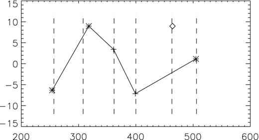
Mode trapping

Fig. 4 presents the residuals to the linear fit for the periods of three m = 0 modes, together with the residuals corresponding to the periods of the undetected m = 0 modes in Table 5. The missing central periods for the two doublets are also plotted, and the period of the single mode point is shown as open circle. From Fig. 4, a possible trapped mode could be visible for the period around 400 s.

Figure 4.

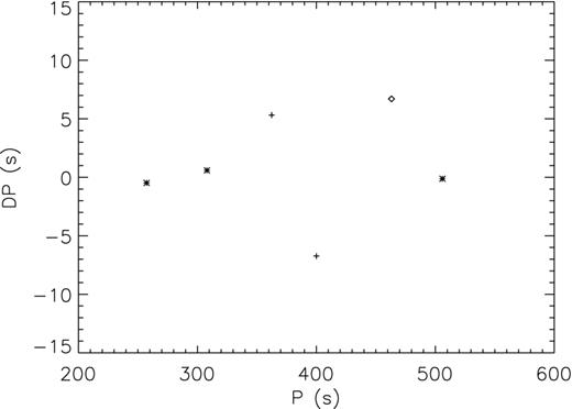
Residuals (DP) of the linear fit to the periods of three m = 0 modes (star mark) versus the period. The residuals corresponding to the periods of the undetected m = 0 modes in the two doublets are also plotted with cross marks, the period of the single mode is shown as an open circle.

Open in new tab Download slide

AMPLITUDE VARIATIONS

As mentioned before, KUV 08368+4026 shows a varying amplitude spectra in different observation seasons. The variations are in the scales of not only years but also weeks. Table 6 lists the amplitudes and their uncertainties from Monte Carlo simulations of the 25 frequencies resolved in data set 3 in the three individual weeks from 2009 December to 2010 January. Fig. 5 shows the amplitude changes of each frequency in the three individual weeks. The amplitudes of these frequencies change a lot in a duration of around one month. The variations of large amplitude frequencies are more significant than the low amplitude frequencies. We also calculate the total power for each week using the following equation:

\begin{equation*} {\rm {Total\, Power}}\;{E}=\sum _i A_i^2F_i \end{equation*}

which are listed in the bottom of Table 6. As one may see, the total power of oscillation are changing in different weeks.

Figure 5.

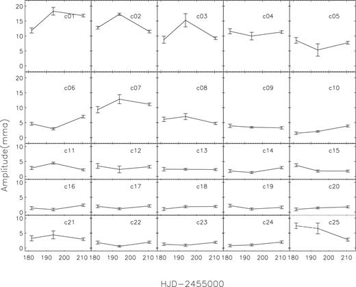
Amplitude variation of the 25 frequencies resolved in data set 3 in different weeks.

Open in new tab Download slide

Table 6.

Open in new tab

The amplitudes list in the three weeks of Data set 3. f is the frequency in μHz. A is the amplitude in mma. Week1 is 2009 Dec. 12–18, Week2 is 2009 Dec. 26–31, 2010 Week3 is Jan. 07–19. E is the total power of oscillation in mma² s⁻¹.

ID	f	Week1	Week2	Week3
		A±σ
c16	747.51	1.20 ± 0.52	0.86 ± 0.42	2.43 ± 0.42
c22	875.50	1.69 ± 0.49	0.34 ± 0.29	1.85 ± 0.29
c20	1127.55	0.82 ± 0.47	1.47 ± 0.30	1.73 ± 0.30
c15	1270.98	3.77 ± 0.52	1.80 ± 0.35	1.73 ± 0.35
c13	1387.15	2.35 ± 0.60	2.35 ± 0.32	2.30 ± 0.32
c21	1975.43	3.12 ± 0.87	4.4 ± 1.3	2.9 ± 1.3
c05	1976.44	8.51 ± 0.94	5.0 ± 2.1	7.6 ± 2.1
c12	1977.42	3.44 ± 0.80	1.6 ± 1.1	3.2 ± 1.1
c14	2159.25	1.59 ± 0.49	1.24 ± 0.35	2.88 ± 0.35
c02	2498.91	12.75 ± 0.45	18.22 ± 0.36	11.54 ± 0.36
c06	2500.62	4.46 ± 0.48	2.90 ± 0.39	6.99 ± 0.39
c11	2758.44	2.84 ± 0.52	4.39 ± 0.36	2.22 ± 0.36
c10	2760.33	1.43 ± 0.42	2.02 ± 0.28	3.89 ± 0.28
c01	3246.39	11.89 ± 0.85	18.2 ± 1.3	16.7 ± 1.3
c25	3247.29	7.27 ± 0.93	6.3 ± 1.8	2.8 ± 1.8
c08	3248.56	6.24 ± 0.73	6.9 ± 1.0	4.7 ± 1.0
c04	3886.01	11.63 ± 0.85	9.8 ± 1.3	11.3 ± 1.3
c03	3887.13	8.6 ± 1.2	15.4 ± 2.2	9.1 ± 2.2
c07	3888.02	9.2 ± 1.1	13.0 ± 1.5	11.1 ± 1.5
c23	5747.48	1.22 ± 0.43	0.81 ± 0.39	1.86 ± 0.39
c19	5863.48	2.05 ± 0.46	1.01 ± 0.37	1.53 ± 0.37
c18	6385.99	0.96 ± 0.50	1.83 ± 0.37	1.88 ± 0.37
c24	6492.81	0.49 ± 0.39	0.89 ± 0.34	1.93 ± 0.34
c09	7134.27	3.90 ± 0.59	3.39 ± 0.27	3.22 ± 0.27
c17	7774.06	1.82 ± 0.45	1.15 ± 0.34	1.99 ± 0.34
			E
		2.823	4.416	3.233

ID	f	Week1	Week2	Week3
		A±σ
c16	747.51	1.20 ± 0.52	0.86 ± 0.42	2.43 ± 0.42
c22	875.50	1.69 ± 0.49	0.34 ± 0.29	1.85 ± 0.29
c20	1127.55	0.82 ± 0.47	1.47 ± 0.30	1.73 ± 0.30
c15	1270.98	3.77 ± 0.52	1.80 ± 0.35	1.73 ± 0.35
c13	1387.15	2.35 ± 0.60	2.35 ± 0.32	2.30 ± 0.32
c21	1975.43	3.12 ± 0.87	4.4 ± 1.3	2.9 ± 1.3
c05	1976.44	8.51 ± 0.94	5.0 ± 2.1	7.6 ± 2.1
c12	1977.42	3.44 ± 0.80	1.6 ± 1.1	3.2 ± 1.1
c14	2159.25	1.59 ± 0.49	1.24 ± 0.35	2.88 ± 0.35
c02	2498.91	12.75 ± 0.45	18.22 ± 0.36	11.54 ± 0.36
c06	2500.62	4.46 ± 0.48	2.90 ± 0.39	6.99 ± 0.39
c11	2758.44	2.84 ± 0.52	4.39 ± 0.36	2.22 ± 0.36
c10	2760.33	1.43 ± 0.42	2.02 ± 0.28	3.89 ± 0.28
c01	3246.39	11.89 ± 0.85	18.2 ± 1.3	16.7 ± 1.3
c25	3247.29	7.27 ± 0.93	6.3 ± 1.8	2.8 ± 1.8
c08	3248.56	6.24 ± 0.73	6.9 ± 1.0	4.7 ± 1.0
c04	3886.01	11.63 ± 0.85	9.8 ± 1.3	11.3 ± 1.3
c03	3887.13	8.6 ± 1.2	15.4 ± 2.2	9.1 ± 2.2
c07	3888.02	9.2 ± 1.1	13.0 ± 1.5	11.1 ± 1.5
c23	5747.48	1.22 ± 0.43	0.81 ± 0.39	1.86 ± 0.39
c19	5863.48	2.05 ± 0.46	1.01 ± 0.37	1.53 ± 0.37
c18	6385.99	0.96 ± 0.50	1.83 ± 0.37	1.88 ± 0.37
c24	6492.81	0.49 ± 0.39	0.89 ± 0.34	1.93 ± 0.34
c09	7134.27	3.90 ± 0.59	3.39 ± 0.27	3.22 ± 0.27
c17	7774.06	1.82 ± 0.45	1.15 ± 0.34	1.99 ± 0.34
			E
		2.823	4.416	3.233

Table 6.

Open in new tab

The amplitudes list in the three weeks of Data set 3. f is the frequency in μHz. A is the amplitude in mma. Week1 is 2009 Dec. 12–18, Week2 is 2009 Dec. 26–31, 2010 Week3 is Jan. 07–19. E is the total power of oscillation in mma² s⁻¹.

ID	f	Week1	Week2	Week3
		A±σ
c16	747.51	1.20 ± 0.52	0.86 ± 0.42	2.43 ± 0.42
c22	875.50	1.69 ± 0.49	0.34 ± 0.29	1.85 ± 0.29
c20	1127.55	0.82 ± 0.47	1.47 ± 0.30	1.73 ± 0.30
c15	1270.98	3.77 ± 0.52	1.80 ± 0.35	1.73 ± 0.35
c13	1387.15	2.35 ± 0.60	2.35 ± 0.32	2.30 ± 0.32
c21	1975.43	3.12 ± 0.87	4.4 ± 1.3	2.9 ± 1.3
c05	1976.44	8.51 ± 0.94	5.0 ± 2.1	7.6 ± 2.1
c12	1977.42	3.44 ± 0.80	1.6 ± 1.1	3.2 ± 1.1
c14	2159.25	1.59 ± 0.49	1.24 ± 0.35	2.88 ± 0.35
c02	2498.91	12.75 ± 0.45	18.22 ± 0.36	11.54 ± 0.36
c06	2500.62	4.46 ± 0.48	2.90 ± 0.39	6.99 ± 0.39
c11	2758.44	2.84 ± 0.52	4.39 ± 0.36	2.22 ± 0.36
c10	2760.33	1.43 ± 0.42	2.02 ± 0.28	3.89 ± 0.28
c01	3246.39	11.89 ± 0.85	18.2 ± 1.3	16.7 ± 1.3
c25	3247.29	7.27 ± 0.93	6.3 ± 1.8	2.8 ± 1.8
c08	3248.56	6.24 ± 0.73	6.9 ± 1.0	4.7 ± 1.0
c04	3886.01	11.63 ± 0.85	9.8 ± 1.3	11.3 ± 1.3
c03	3887.13	8.6 ± 1.2	15.4 ± 2.2	9.1 ± 2.2
c07	3888.02	9.2 ± 1.1	13.0 ± 1.5	11.1 ± 1.5
c23	5747.48	1.22 ± 0.43	0.81 ± 0.39	1.86 ± 0.39
c19	5863.48	2.05 ± 0.46	1.01 ± 0.37	1.53 ± 0.37
c18	6385.99	0.96 ± 0.50	1.83 ± 0.37	1.88 ± 0.37
c24	6492.81	0.49 ± 0.39	0.89 ± 0.34	1.93 ± 0.34
c09	7134.27	3.90 ± 0.59	3.39 ± 0.27	3.22 ± 0.27
c17	7774.06	1.82 ± 0.45	1.15 ± 0.34	1.99 ± 0.34
			E
		2.823	4.416	3.233

ID	f	Week1	Week2	Week3
		A±σ
c16	747.51	1.20 ± 0.52	0.86 ± 0.42	2.43 ± 0.42
c22	875.50	1.69 ± 0.49	0.34 ± 0.29	1.85 ± 0.29
c20	1127.55	0.82 ± 0.47	1.47 ± 0.30	1.73 ± 0.30
c15	1270.98	3.77 ± 0.52	1.80 ± 0.35	1.73 ± 0.35
c13	1387.15	2.35 ± 0.60	2.35 ± 0.32	2.30 ± 0.32
c21	1975.43	3.12 ± 0.87	4.4 ± 1.3	2.9 ± 1.3
c05	1976.44	8.51 ± 0.94	5.0 ± 2.1	7.6 ± 2.1
c12	1977.42	3.44 ± 0.80	1.6 ± 1.1	3.2 ± 1.1
c14	2159.25	1.59 ± 0.49	1.24 ± 0.35	2.88 ± 0.35
c02	2498.91	12.75 ± 0.45	18.22 ± 0.36	11.54 ± 0.36
c06	2500.62	4.46 ± 0.48	2.90 ± 0.39	6.99 ± 0.39
c11	2758.44	2.84 ± 0.52	4.39 ± 0.36	2.22 ± 0.36
c10	2760.33	1.43 ± 0.42	2.02 ± 0.28	3.89 ± 0.28
c01	3246.39	11.89 ± 0.85	18.2 ± 1.3	16.7 ± 1.3
c25	3247.29	7.27 ± 0.93	6.3 ± 1.8	2.8 ± 1.8
c08	3248.56	6.24 ± 0.73	6.9 ± 1.0	4.7 ± 1.0
c04	3886.01	11.63 ± 0.85	9.8 ± 1.3	11.3 ± 1.3
c03	3887.13	8.6 ± 1.2	15.4 ± 2.2	9.1 ± 2.2
c07	3888.02	9.2 ± 1.1	13.0 ± 1.5	11.1 ± 1.5
c23	5747.48	1.22 ± 0.43	0.81 ± 0.39	1.86 ± 0.39
c19	5863.48	2.05 ± 0.46	1.01 ± 0.37	1.53 ± 0.37
c18	6385.99	0.96 ± 0.50	1.83 ± 0.37	1.88 ± 0.37
c24	6492.81	0.49 ± 0.39	0.89 ± 0.34	1.93 ± 0.34
c09	7134.27	3.90 ± 0.59	3.39 ± 0.27	3.22 ± 0.27
c17	7774.06	1.82 ± 0.45	1.15 ± 0.34	1.99 ± 0.34
			E
		2.823	4.416	3.233

MODELING EXPLORATION

We used the theoretical static models calculated with the Toulouse white dwarf code (Pech et al. 2006) to constrain the stellar parameters of KUV 08368+4026. The models have four input parameters, total mass, luminosity, hydrogen mass fraction and helium mass fraction. First, we built a large grid in a large parameter range to select potential good-fit models. The ranges and steps of the grid are listed in Table 7. χ² test estimates were used to find the best-fitting models with the five l = 1 modes and the l = 2 mode.

\begin{equation*} \chi ^2=\sum _n(P^{\rm the}_n-P^{\rm obs}_n)^2, \end{equation*}

where P^the are the periods of theoretical models and P^obs are observing periods.

Table 7.

Open in new tab

Parameters of the large grid.

	Range	Step
Mass ( M_⊙)	0.60–0.84	0.01
Luminosity (L_⊙)	2.0 ∼ 4.5 × 10⁻³	0.1 × 10⁻³
log M_H/M_★	−3.5 ∼ −10	0.5
log M_He/M_★	−2

Table 7.

Open in new tab

Parameters of the large grid.

	Range	Step
Mass ( M_⊙)	0.60–0.84	0.01
Luminosity (L_⊙)	2.0 ∼ 4.5 × 10⁻³	0.1 × 10⁻³
log M_H/M_★	−3.5 ∼ −10	0.5
log M_He/M_★	−2

More than 8000 models are calculated for the large grid. We constrain the parameters with the effective temperature and the surface gravity from Gianninas et al. (2011) catalogue and Fontaine et al. (2003). We selected the models whose parameters locate inside the range of three times uncertainty of the parameters and one minimum of χ² was found among the models. Around it we build a detailed grid to get more precise parameters. Table 8 lists the range of the detailed grid. The value of the hydrogen mass fraction was fixed to 10^−4.0 because we notice the fact that the models with larger hydrogen mass fraction fit the observing modes better in the large grid.

Table 8.

Open in new tab

Parameters of the detailed grid.

	Ranges	Steps
Mass ( M_⊙)	0.67–0.71	0.002
Luminosity (L_⊙)	2.7 ∼ 3.1 × 10⁻³	0.02 × 10⁻³
log M_H/M_★	−4.0
\|$\log M_{\text{He}/M_*}$\|	−2

Table 8.

Open in new tab

Parameters of the detailed grid.

	Ranges	Steps
Mass ( M_⊙)	0.67–0.71	0.002
Luminosity (L_⊙)	2.7 ∼ 3.1 × 10⁻³	0.02 × 10⁻³
log M_H/M_★	−4.0
\|$\log M_{\text{He}/M_*}$\|	−2

Fig. 6 displays the distribution of χ² test of the six multiple mode calculated from models and the observed mode. The χ² values of 100 000/χ² are represented by different grey-scales. One minimum was found and the model was identified as the best-fitting model. Table 9 presents the parameters of the best-fitting model.

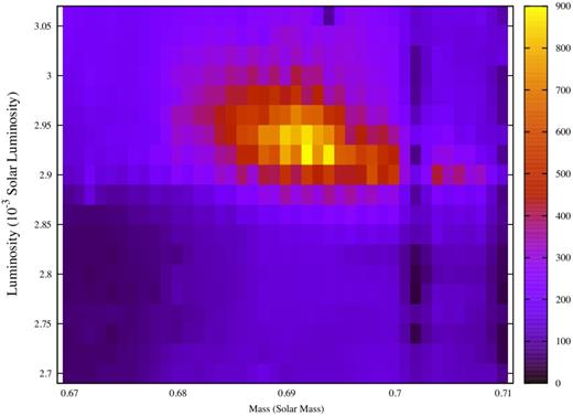
χ2 test of the detailed grids. The grey-scales present the value of 100 000/χ2.

Figure 6.

χ² test of the detailed grids. The grey-scales present the value of 100 000/χ².

Open in new tab Download slide

Table 9.

Open in new tab

Parameter of best-fitting model for KUV 08368+4026.

T_eff(K)

11 825.1

log g

8.06

L(L_⊙)

(2.92 ± 0.02) × 10⁻³

M(M_⊙)

0.692 ± 0.002

M_H/M_★

10⁻⁴

M_He/M_★

10⁻²

We tried to do analysis for the trapped modes of the best-fitting model and the result is presented in Fig. 7.

Figure 7.

Mode trapping analysis of the seven best-fitting models. The symbols are the same as Fig. 4.

Open in new tab Download slide

We suggest to take this model as the best-fitting model for the following reasons: (1) it has the closest pulsation modes to the observation modes; (2) it shows a trapped mode around the 400 s period, which agrees with the observation; (3) the effective temperature and surface gravity of this model locate between the values given by the two spectroscopic observation efforts. Therefore, we take it as the best-fitting model under the current condition.

DISCUSSION AND CONCLUSIONS

We summarize our work as follows.

We obtained time series photometric data for the ZZ Ceti star KUV 08368+4026 in 1999 and from 2009 to 2012. 17 independent modes were extracted, including six multiplets and one single mode together with 13 (f18–30) further signals. We identified the independent signals as either l = 1 or l = 2 modes from the rotational splitting. Also a number of linear combinations and low amplitude modes are resolved but we failed to identify them.
From the six multiplets, an average rotational splitting of 1.049 ± 0.041 μHz was determined which derived the rotation period of 5.52 ± 0.22 d.
An average period spacing of 49.2 s was obtained from the l = 1, m = 0 modes.
The 1998 campaign (Dolez et al. 1999) reports six independent frequencies but no rotation splitting was detected due to the observation conditions. The six frequencies matches the six multiplets presented in this work exactly. This campaign gave a period spacing of 52 s base on five modes which were defined as l = 1 modes from our work and derived a mass of 0.6 M_⊙ for KUV 08368+4026, a little larger than our constraints. The two periods of 619 and 494.5 s found in the discovery observation were not detected in neither 1998 campaign nor the following observations.
We found the evidence of amplitude variations of KUV 08368+4026 in time-scale of both years and weeks. The total pulsation power was changing as well in the three weeks from 2009 December tot 2010 January.
The theoretical modelling work suggests a thick hydrogen layer for KUV 08368+4026. We estimate a best-fitting model with a mass of 0.692 ± 0.002 M_⊙, luminosity of (2.92 ± 0.02) × 10⁻³ L_⊙ and hydrogen mass fraction of 10⁻⁴ stellar mass and helium mass fraction of 10⁻² stellar mass
Romero et al. (2012) gave a set of stellar parameters from their theoretical modelling work which suggested log g of 8.02 ± 0.03, mass of 0.609 ± 0.012 M_⊙, effective temperature of 11230 ± 95K, M_H/M_★ of (1.42 ± 0.52) × 10⁻⁵ and M_He/M_★ of 2.45 × 10⁻² based on the only two periods of the discovery data. Thus our constraints, which are based on more data from multisite campaigns should be considered as more reliable.

CL and JNF acknowledge the support from the Joint Fund of Astronomy of National Natural Science Foundation of China (NSFC) and Chinese Academy of Sciences through the Grant U1231202, and the support from the National Basic Research Program of China (973 Program 2014CB845701 and 2013CB834904). LFM acknowledges the financial support from the UNAM under grant PAPIIT IN105115. MC would like to thank CONACyT for financial support though grant 134985.

★

Based on data obtained at the Xinglong station of National Astronomical Observatories of China, the Lijiang station of Yunnan Astronomical Observatory, China, the San Pedro Martir Observatory, Mexico, the Observatorio Astrofisico Guillermo Halo, Mexico, and the Observatoire de Haute Provence, France.

REFERENCES

Brickhill

A. J.

,

MNRAS

,

1975

, vol.

170

pg.

404

Crossref

Search ADS

Dolez

N.

Vauclair

G.

Zhang

X. B.

Chevreton

M.

Handler

G.

Solheim

S.-E.

Meistas

E. G.

,

ASP Conf. Ser. Vol. 169, 11th European Workshop on White Dwarfs

,

1999

San Francisco

Astron. Soc. Pac.

pg.

129

Google Scholar

Google Preview

OpenURL Placeholder Text

WorldCat

Fontaine

G.

Bergeron

P.

Billères

M.

Charpinet

S.

,

ApJ

,

2003

, vol.

591

pg.

1184

Crossref

Search ADS

Fu

J.-N.

et al. ,

MNRAS

,

2013

, vol.

429

pg.

1585

Crossref

Search ADS

Gianninas

A.

Bergeron

P.

Ruiz

M. T.

,

ApJ

,

2011

, vol.

743

pg.

138

Crossref

Search ADS

Landolt

A. U.

,

ApJ

,

1968

, vol.

153

pg.

151

Crossref

Search ADS

Lenz

P.

Breger

M.

,

Commun. Asteroseismol.

,

2005

, vol.

146

pg.

53

Crossref

Search ADS

Pech

D.

Vauclair

G.

Dolez

N.

,

A&A

,

2006

, vol.

446

pg.

223

Crossref

Search ADS

Romero

A. D.

Górsico

A. H.

Althaus

L. G.

Kepler

S. O.

Castanheira

B. G.

Miller

Bertolami M. M.

,

MNRAS

,

2012

, vol.

420

pg.

1462

Crossref

Search ADS

Vauclair

G.

Dolez

N.

Fu

J.-N.

Chevreton

M.

,

A&A

,

1997

, vol.

322

pg.

155

Winget

D. E.

Hansen

C. J.

Liebert

J.

van Horn

H. M.

Fontaine

G.

Nather

R. E.

Kepler

S. O.

Lamb

D. Q.

,

ApJ

,

1987

, vol.

315

pg.

77

Crossref

Search ADS

Download all slides

Month:	Total Views:
November 2016	1
January 2017	4
February 2017	10
March 2017	3
April 2017	2
June 2017	1
July 2017	2
August 2017	1
September 2017	2
October 2017	1
February 2018	3
March 2018	3
April 2018	3
May 2018	3
June 2018	10
July 2018	10
August 2018	8
September 2018	5
October 2018	2
November 2018	2
December 2018	5
January 2019	5
February 2019	4
March 2019	6
April 2019	10
May 2019	9
June 2019	6
July 2019	4
August 2019	5
September 2019	1
October 2019	7
November 2019	6
December 2019	3
January 2020	6
February 2020	8
March 2020	8
April 2020	3
May 2020	3
June 2020	4
July 2020	4
August 2020	3
September 2020	4
October 2020	3
November 2020	3
January 2021	5
February 2021	2
March 2021	7
April 2021	3
May 2021	1
July 2021	1
August 2021	3
September 2021	2
October 2021	3
November 2021	3
January 2022	1
February 2022	7
March 2022	2
April 2022	7
May 2022	1
June 2022	2
July 2022	12
August 2022	11
September 2022	9
October 2022	8
November 2022	4
December 2022	9
January 2023	1
February 2023	4
March 2023	1
April 2023	7
May 2023	7
August 2023	3
September 2023	3
October 2023	2
November 2023	3
December 2023	7
January 2024	12
February 2024	22
March 2024	5
April 2024	5
May 2024	3
June 2024	6
July 2024	6
August 2024	6
September 2024	4
October 2024	9
November 2024	25
December 2024	3
January 2025	4
February 2025	3
March 2025	29
April 2025	1
May 2025	11

Article Contents

Asteroseismology of the ZZ Ceti star KUV 08368+4026^★

Abstract

INTRODUCTION

OBSERVATIONS AND DATA REDUCTION

PERIOD ANALYSIS

ASTEROSEISMOLOGY

Linear combinations

Mode identification

Rotational splitting

Period spacing

Mode trapping

AMPLITUDE VARIATIONS

MODELING EXPLORATION

DISCUSSION AND CONCLUSIONS

REFERENCES

Citations

Views

Altmetric

Email alerts

Astrophysics Data System

Citing articles via

Latest

Most Read

Most Cited

Article Contents

Asteroseismology of the ZZ Ceti star KUV 08368+4026★ Free

Abstract

INTRODUCTION

OBSERVATIONS AND DATA REDUCTION

PERIOD ANALYSIS

ASTEROSEISMOLOGY

Linear combinations

Mode identification

Rotational splitting

Period spacing

Mode trapping

AMPLITUDE VARIATIONS

MODELING EXPLORATION

DISCUSSION AND CONCLUSIONS

REFERENCES

Citations

Views

Altmetric

Email alerts

Astrophysics Data System

Citing articles via

Latest

Most Read

Most Cited

This Feature Is Available To Subscribers Only

Asteroseismology of the ZZ Ceti star KUV 08368+4026^★