


Abstract
We report the results of a multiwaveband analysis of the masses and luminosities of ∼600 galaxy groups and clusters identified in the maxBCG catalogue. These data are intended to form the basis of future work on the formation of the ‘m12 gap’ in galaxy groups and clusters. We use SDSS spectroscopy and g-, r- and i-band photometry to estimate galaxy group/cluster virial radii, masses and total luminosities. In order to establish the robustness of our results, we compare them with literature studies that utilize a variety of mass determinations techniques (dynamical, X-ray and weak lensing) and total luminosities estimated in the B, r, i and K wavebands. We also compare our results to predictions derived from the Millennium Simulation. We find that, once selection effects are properly accounted for, excellent agreement exists between our results and the literature with the exception of a single observational study. We also find that the Millennium Simulation does an excellent job of predicting the effects of our selection criteria. Our results show that, over the mass range ∼1013–1015 M⊙, variations in the slope of the mass–luminosity scaling relation with mass detected in this and many other literature studies is in part the result of selection effects. We show that this can have serious ramifications on attempts to determine how the mass-to-light ratio of galaxy groups and cluster varies with mass.
1 INTRODUCTION
In 1933, Fritz Zwicky applied the virial theorem to a galaxy cluster (the Coma cluster) for the first time (Zwicky 1933). He concluded that, in order to explain the cluster's dynamics, the average density of the cluster had to be several hundred times greater than that indicated by estimates of the mass of luminous material observed in the cluster's galaxies alone. Confirmed later in the Virgo cluster (Smith 1936), these were, of course, the first direct observations indicating the presence of dark matter (Zwicky's ‘Dunkle Materie’).
Zwicky's methodology of measuring the mass of clusters and comparing this mass to the total light emitted by the galaxies in the cluster is still in use today. Indeed, the measurement of mass-to-light ratios in galaxy groups and clusters has become commonplace since these discoveries, as knowledge of how the mass of baryonic and non-baryonic matter are distributed within clusters provide important clues as to how they, and the galaxies within them, were formed.
However, the techniques and data involved in measuring both the masses and luminosities of clusters have become significantly more sophisticated since Zwicky's original discovery. For instance, with the coming of large telescopes and large-scale surveys, the measurement of group/cluster luminosities has advanced, permitting direct observation of galaxies further down the luminosity function and to higher redshifts, while mass estimates can now be based upon cluster dynamics (as performed by Zwicky and Smith), or in more recent advances, X-ray properties of cluster haloes or gravitational lensing. However, due to the variations in methodologies adopted in works in the literature, the received wisdom has become that it is difficult to make direct comparisons between studies.
In this work we examine this issue, comparing the results of our analysis of the masses and luminosities of ∼600 galaxy groups and clusters identified in the maxBCG catalogue with the results of the Millennium Simulation (MS) and five other recent studies in the literature that use a variety of methodologies and data sources. Our analysis is performed in four wavebands (B, r, i and K) and includes systems of mass ranging from ∼1013 to 1015 M⊙. We examine both the extensive areas of agreement, as well as areas of disagreement, between these studies and identify the issues that must be considered before making comparisons between studies.
In future papers, we will use the data presented here to perform an analysis aimed at identifying the group/cluster properties driving differences in the ‘m12 gap’ (the luminosity difference between the brightest and second brightest galaxies within the central regions of groups and clusters).
Throughout this paper both our data and literature data are presented assuming a H0 = 70 km s−1 Mpc−1, ΩΛ = 0.7 and ΩM = 0.3 cosmology. For expressing luminosities in solar units, we used the values Mr, ⊙ = 4.67 mag, Mi, ⊙ = 4.48 mag, MB, ⊙ = 5.33 mag and MK, ⊙ = 3.28 mag.
2 DATA
Our sample was selected from groups identified in the maxBCG catalogue of Koester et al. (2007b). This catalogue was constructed from the SDSS photometric survey using a cluster finding algorithm based on three well-defined properties of galaxies in clusters: spatial clustering, the presence of a ‘red-sequence’ and the presence of a brightest cluster galaxy(BCG) at the centre of the cluster (Koester et al. 2007a). Using this method, Koester et al. (2007b) identify more than 13 000 clusters. Using DR9 of the SDSS-III (Ahn et al. 2012), we then selected all the clusters from the maxBCG catalogue that have a BCG with a spectroscopic redshift in the redshift interval z = 0.05–0.16 and possessing six or more spectroscopically confirmed members (as described in Section 2.3).
The upper end of the selected redshift range was chosen in order to ensure a substantive sample at all values of the ‘m12 gap’, as it is necessary to probe out to redshifts of ∼0.15 in order to obtain a reasonably large sample of the rare ‘fossil groups’ (defined as systems with m12 > 2). The lower end of the redshift range was chosen to minimize the impact of the redshift dependent selection criteria of the SDSS spectroscopic survey which only sampled galaxies with apparent magnitude brighter than 17.7 mag in the r band, and to ensure that the peculiar velocities of the groups and clusters studied have minimal impact on distance determinations and their associated distance moduli, and thus ensuring accurate luminosity estimates. A minimum of six spectroscopically confirmed members were required as the mass estimates made in this work are based on velocity dispersion estimates whose errors are large when the number of spectroscopically confirmed members is low. Indeed, even with a sample of six spectroscopically confirmed members, errors in log(mass) estimates are of the order of 0.4 dex (or a factor of 2.5 in mass).
2.1 Data from the literature
In this work, we compare our results to those of five recent studies. These studies are: Girardi et al. (2002), Eke et al. (2004b), Ramella et al. (2004), Popesso et al. (2007) and Sheldon et al. (2009). These studies span four wavebands (B, r, i and K). In each case, the results of these studies were, if necessary, converted to the H0 = 70 km s−1 Mpc−1, ΩΛ = 0.7, ΩM = 0.3 cosmology used throughout this paper. Where necessary, small corrections were also made to ensure that the same solar luminosities were used in the estimation of group/cluster luminosities and that the data are k-corrected to the same redshift (z = 0). We note that the literature studies above are generally based on groups/clusters at lower redshift than our data, and a minimum of 10 spectroscopically confirmed members are generally applied (rather than the six used here). The studies using dynamical mass estimates therefore generally possess average mass errors that are smaller than ours by, in the worst case, ∼0.1 dex.
2.2 The MS
To supplement our analysis and provide a means of testing the impact on observations of errors and selection effects, we also use the galaxy recession velocities (for dynamical mass estimation) and luminosity data from the Millennium Run dark matter simulation in the Wilkinson Microwave Anisotropy Probe cosmology (H0 = 73 km s−1 Mpc−1, ΩΛ = 0.75, and ΩM = 0.25) from Springel et al. (2005), together with the semi-analytic galaxy modelling technique as described in Guo et al. (2011). The semi-analytic galaxy catalogues were converted into an observer's light-cone geometry matched to the SDSS survey by Henriques et al. (2012) using the models of Bruzual & Charlot (2003), assuming a Chabrier (2003) initial mass function. Henriques et al. (2012) estimated total luminosities in a broad range of photometric bands from the B band to the infrared. In this work, we use the r band data only. These data were converted to the H0 = 70 km s−1 Mpc−1 cosmology used throughout this paper. The corrections for ΩΛ and ΩM were deemed insignificant for this work as they cause differences of only ∼0.01 mag and ∼0.4 per cent in the distance moduli and angular sizes, respectively. Data for all galaxies brighter than 22 mag in the r band (the photometric limit of the SDSS data used in our analysis) in simulated haloes at redshifts less than 0.16 were obtained, and the positions and r band luminosities of each galaxy, along with the M200 of the parent haloes, were tabulated.
2.3 Spectroscopic selection and analysis
We then searched the SDSS spectroscopic catalogue for all galaxies within the estimated R200 that possess redshifts differing from the BCG redshift by less than 1500 km s−1 (i.e. ±2.5σ). The value 2.5σ was selected in order to allow for the inherent scatter expected from the (almost Gaussian) distribution of velocities observed in clusters, while at the same time minimizing the likelihood of selecting interlopers. Once all the members within R200 were identified their redshifts were used to calculate a new velocity dispersion using the Beers, Flynn & Gebhardt (1990) biweight estimator for systems with more than 10 members, and the Beers et al. (1990) gapper method for systems with 10 or less members. For cases where the initial velocity dispersions were an underestimate this resulted in an increase in the velocity dispersion (and hence R200) estimate, as well as increasing the permitted velocity range (±2.5σnew). Conversely, for systems in which the initial values were an overestimate the new values were lower. This process was iterated a number of times. We found that, generally, convergence was achieved after only two or three iterations. However, a total of 10 iterations were performed. This permitted the use of the value from the last (10th) iteration as the final result for each group/cluster, while the rms scatter in the last six iterations was taken as an additional uncertainty in the velocity dispersion and which was added in quadrature to the formal velocity dispersion error. We note that this additional error is zero for the majority of systems in which the procedure converged.
At this stage, groups/clusters with less than six spectroscopically confirmed members within R200 were discarded from the sample. Clusters for which the average recession velocity of all the galaxies except the BCG differed from the recession velocity of the BCG by more than 400 km s−1 were also excluded, as these have a high probability of being either highly disturbed (i.e. non-virialized) systems or false/contaminated detections due to line-of-sight effects.
2.4 Mass estimation
However, it is helpful to note that log(E(z)) is small (∼0.02 at the z = 0.1 median of the data presented here) and varies by only ±0.02 over the whole redshift range of the clusters reported here. The resultant masses spanned the range from ∼1013 to ∼1015 M⊙.
We note that four of the five literature studies to which we compare our results (Girardi et al. 2002; Eke et al. 2004b; Ramella et al. 2004; Popesso et al. 2007) use equation (2) to estimate masses. However, both Girardi et al. (2002) and Popesso et al. (2007) make corrections for a surface pressure term. A comparison of the masses presented in Girardi et al. (2002) with masses estimated using their velocity dispersions and equation (2) yields an offset of 0.00 dex with rms scatter of only 0.12 dex. This demonstrates that this term is small and of no significance to the results presented here. Eke et al. (2004b), on the other hand, use the spatial distribution of the galaxies in each system to estimate R200 rather than equation (1), basing their values of radius on a calibration against cosmological simulations (Eke et al. 2004a).1 Finally, Sheldon et al. (2009) utilize SDSS i-band photometry and masses derived from weak gravitational lensing.
As a first test of our dynamical mass estimates, we performed a search of the literature for groups/clusters in our study for which masses derived from X-ray properties have either been reported or can be estimated. A total of 24 groups from our study were found to have masses based on a variety of X-ray properties reported in the literature (Donahue et al. 2005; Jia, Chen & Chen 2006; Lemze et al. 2008; Zibetti, Pierini & Pratt 2009; Akamatsu et al. 2011; Proctor et al. 2011; Miller et al. 2012; Owers et al. 2014). For the majority of these studies (Donahue et al. 2005; Zibetti et al. 2009; Akamatsu et al. 2011; Proctor et al. 2011; Miller et al. 2012; Owers et al. 2014), X-ray masses were estimated from X-ray temperature using the Tier 1 relation from Sun et al. (2009, their table 6). However, the X-ray masses taken from Jia et al. (2006) were derived using X-ray temperature and electron density, while in the case of Lemze et al. (2008), weak lensing and the X-ray luminosity profile were employed to determine cluster masses. The masses derived from all the above studies assume hydrostatic equilibrium.
The results of the comparison of dynamical masses to those derived from X-ray data are shown as solid points in Fig. 1. Also shown in this figure as open squares are total cluster masses derived from Zhang et al. (2011) X-ray gas masses assuming the relation derived by Mahdavi et al. (2013) between X-ray gas masses and total cluster masses. This relation was calibrated by comparing gas masses from X-ray analyses to the results of total cluster masses from weak lensing. Dynamical masses for these data were derived using the velocity dispersions provided in Zhang et al. (2011) and equation (3). Velocity dispersions and masses derived from X-ray temperature were also taken from Osmond & Ponman (2004) and Wu, Xue & Fang (1999). For these data, dynamical masses were derived using equation (3), while X-ray masses were derived from the X-ray temperatures using Sun et al. (2009) as above. The results of Osmond & Ponman (2004) and Wu et al. (1999) are shown in Fig. 1 as open circles and triangles, respectively. Again, hydrostatic equilibrium is assumed in all cases, and all the above results are for masses within R200. Where necessary, we assumed that R200 = 1.54R500, consistent with the values of R200 and R500 for clusters given in Ettori et al. (2010), yielding M200 = 1.46M500.
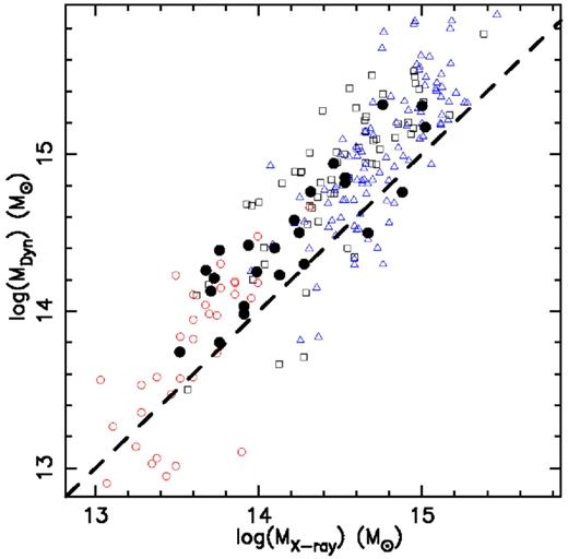
Comparison of dynamical mass, estimated as detailed in the text, with masses derived from X-ray data. Black dots are clusters in our study (whose dynamical masses are estimated here) with X-ray masses from the literature. Open squares are derived from the velocity dispersion and X-ray gas mass data from Zhang et al. (2011, see text). Open circles and triangles are derived from the velocity dispersion and X-ray temperature data of Osmond & Ponman (2004) and Wu et al. (1999), respectively. The dashed line shows the one-to-one locus. At masses greater than ∼1014 M⊙ there is a clear, constant offset between X-ray and dynamical masses, while below this mass there is a suggestion of a change in slope in the correlation.
Now, given the inhomogeneity of these data, and the need to convert between M500 and M200, it would be unwise to overinterpret this plot. However, we note that in Fig. 1, systems with masses above ∼1014 M⊙, although running parallel to the one-to-one line, the X-ray masses appear systematically offset from the dynamical masses by ∼0.15 dex. On the other hand, the systems with masses lower than ∼1014 M⊙ (which are from Osmond & Ponman 2004), the data straddle the one-to-one line, but appear to exhibit a slope greater than one. This change in gradient at low masses was noted in Osmond & Ponman (2004) when they considered their LX − σ and σ − TX plots (their sections 7.2 and 7.3) and was also noted in Helsdon & Ponman (2000). A break in the slope of the X-ray scaling relations at a temperature of about 1 keV (corresponding to a mass of ∼1014 M⊙) is also evident in a number of studies (e.g. Xue & Wu 2000 and Harrison et al. 2012). However, it has been disputed in other works, e.g. Mulchaey (2000). Therefore, there remains no real consensus as to whether the apparent change in gradient in the LX − σ and σ − TX scaling relations represents a true physical effect or is rather an artefact of large errors and selection effects in low-mass systems (see Osmond & Ponman 2004, for a more detailed description of the controversy).
It is also interesting to perform a similar comparison using the MS data, in this case comparing dynamical mass to the M200 values given in the data base. The masses presented in the data base were calculated by simply adding the masses of all the particles within the region of each halo where the average density is 200 times the critical density. In order to calculate dynamical masses we applied the same analysis as that applied to our observational data. i.e. assuming that the BCG lay at the centre of the cluster and measuring recession velocities with respect to the central galaxy using the Beers et al. (1990) biweight and gapper estimators as described in Section 2.3 to estimate velocity dispersion. Dynamical masses are then estimated using equation (3). This analysis was performed under the assumption of a variety of selection criteria, including those describing our observational data, which we recall were selected to have redshifts between 0.05 and 0.16, and have six or more members with apparent magnitudes brighter than the 17.7 mag within R200. For each analysis, the median of the dynamical mass data in bins of MS mass were calculated. We note that our use of the median in these analyses ensures that the effects of the asymmetrical errors in dynamical mass are essentially eliminated.
The comparison between MS masses and dynamical masses is shown in Fig. 2. In this plot, the dynamical masses are those for all systems with a minimum of six members, but with no redshift or member luminosity selection limits applied. Reasonable agreement is found. At masses greater than ∼1014 M⊙ the MS masses show an offset from the median dynamical masses of ∼0.1 dex, similar to the trend in the X-ray data in Fig. 1. Below ∼1014 M⊙, the correlation between MMS and MDyn steepens, with the gradient increasing from 1.05 above ∼1014 M⊙ to 1.17 below this mass. Although statistically only marginally (∼2σ) significant, this steepening at low masses is again at least qualitatively similar to the X-ray data. Some care must be taken in the interpretation of these differences, since given the large uncertainties in the semi-analytic models that describe the baryonic physics, there is no guarantee that the MS data match the real Universe in this regard. However, it is interesting to note that offset at high masses and the increased gradient at lower masses are at least qualitatively consistent with the trends in the X-ray data. This therefore raises the possibility that this represents a real systematic bias in dynamical masses, perhaps due to a bias in the distribution of galaxies with respect to the underlying dark matter halo or perhaps representing a breakdown in the assumptions made in deriving dynamical masses (i.e. the assumption of full virialization and/or that the systems are well described as isothermal spheres).
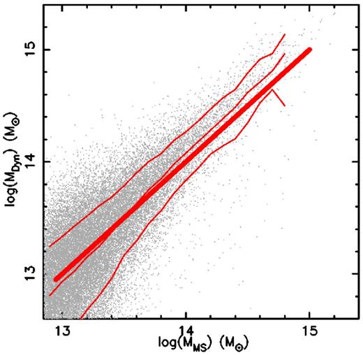
Comparison of masses using our dynamical mass estimation method (see text) with masses from the MS. The thick red line shows the one-to-one locus, while the thin lines show the median and 15/85 percentiles of the dynamical masses in bins of 0.1 dex in MS mass. As well as an offset at high masses, the data exhibit and increase in slope at masses below 1014 M⊙.
2.5 Photometric analysis
Having established estimates of the masses of the clusters in our sample we must next estimate the total luminosity of each of the systems. Therefore, for each of the clusters selected above, the g-, r- and i-band photometry of all galaxies within 4R200 of the BCG were obtained from the SDSS photometric survey. We use the SDSS model magnitudes which were estimated using a combination of De Vaucouleurs and exponential profiles. Galaxies with SDSS spectroscopic redshifts were k-corrected to zero redshift using the colour dependent functions of Chilingarian, Melchior & Zolotukhin (2010).
For each cluster, and in each waveband (g, r and i), the total luminosity of the galaxies within R200 was then estimated in a two step process. First, the luminosities of all the spectroscopically confirmed galaxies within R200 of each group were co-added to derive the total luminosity. Next, the total luminosity of all galaxies in the photometric survey with apparent magnitudes fainter than 17.7 mag in the r band (the lower limit of the spectroscopic survey) and brighter than 22.2 mag (the 95 per cent completeness limit of the photometric survey) were co-added. We note that modelling of the Blanton et al. (2003) SDSS r-band luminosity function indicates that even in our most distant clusters the contribution to the total light of galaxies fainter than our upper limit of 22.2 would be less than 2.5 per cent (i.e. a log(luminosity) = 0.01). This contribution is therefore deemed insignificant to our results, and is ignored.
A colour cut excluding all galaxies 0.2 mag redder in (g − r) than the BCG was applied in order to minimize the impact of contamination by high-redshift interlopers. In order to estimate the background contamination, the same process was applied to seven concentric annuli between 3R200 and 4R200. These annuli were selected to have an area equal to the area of the central region within R200. In each of the g, r and i bands, the median value of the seven annuli was then taken as the background level and this value was subtracted from the value calculated within R200 yielding an estimate of the total luminosity of faint galaxies within R200. These luminosities were also then k-corrected to zero redshift using the functions of Chilingarian et al. (2010). The total luminosity in faint galaxies was then added to the total luminosity in spectroscopically confirmed galaxies to yield a total luminosity for each group.
However, in some cases the background luminosity in faint galaxies exceeded the estimated total luminosity of all the galaxies in the cluster, resulting in negative values for the luminosity of the cluster, clearly indicating that the background level was overestimated. Such clusters were excluded from our analysis. In other cases, despite high background levels, the total luminosities of the clusters remained positive raising the possibility that the clusters had, indeed, very low luminosity compared to the background against which they are projected. In such cases, we excluded only clusters in which the background level exceeded five times the luminosity of faint galaxies in the cluster, deeming the uncertainties in the background level to be too large for a reliable total luminosity estimate.
After all the selection cuts above were made we retained a total of 614 clusters.
In order to compare literature values in the B and K bands, we used the colour dependent functions of Blanton & Roweis (2007, B band) and Yaz et al. (2010, K band) to estimate the luminosities of each galaxy in each cluster in these bands. The total luminosities in the bands were then also estimated as above.
3 RESULTS
In this section, we report our results and compare them to five recent works from the literature that measure masses and luminosity ratios in significant samples of groups/clusters in the B, r, i and K bands (recall that, for our results, r and i are taken directly from the SDSS data base while B and K are generated from the SDSS data using the colour dependent transforms of Blanton & Roweis 2007 and Yaz et al. 2010, respectively). Examples of these results are shown in Table 1. The full table is available online.
An example of the data published online. The ID is that given in the maxBCG catalogue. Velocity dispersion (σ) and its error are given in km s−1. The number of spectrocopically confirmed members are given by n. All masses and luminosities are in solar units. Luminosity errors are not given for the B and K bands as these were derived using functions from the literature (see text). Errors for B and K bands may be estimated, to first order, as the errors in g and i, respectively.
| ID | RA | DEC | z | n | σ | σerr | log(M) | log(M)err | log(LB) | log(Lg) | log(Lg)err | log(Lr) | log(Lr)err | log(Li) | log(Li)err | log(LK) |
|---|---|---|---|---|---|---|---|---|---|---|---|---|---|---|---|---|
| 13 | 213.784 93 | −0.493 25 | 0.138 93 | 21 | 642.4 | 100.3 | 14.630 | 0.205 | 12.270 | 12.339 | 0.148 | 12.490 | 0.135 | 12.581 | 0.148 | 12.927 |
| 22 | 227.552 96 | 33.492 49 | 0.114 26 | 72 | 1076.9 | 90.1 | 15.308 | 0.109 | 12.389 | 12.466 | 0.030 | 12.649 | 0.031 | 12.729 | 0.057 | 13.096 |
| 161 | 127.024 48 | 44.766 75 | 0.144 96 | 8 | 410.6 | 106.0 | 14.045 | 0.344 | 11.902 | 11.986 | 0.126 | 12.150 | 0.114 | 12.228 | 0.149 | 12.666 |
| 193 | 240.367 02 | 53.947 38 | 0.065 44 | 18 | 341.7 | 57.8 | 13.823 | 0.222 | 11.576 | 11.631 | 0.103 | 11.777 | 0.097 | 11.858 | 0.098 | 12.109 |
| 200 | 133.518 88 | 29.053 54 | 0.084 37 | 36 | 606.3 | 72.0 | 14.566 | 0.155 | 11.902 | 11.957 | 0.025 | 12.128 | 0.022 | 12.221 | 0.036 | 12.448 |
| 205 | 224.640 01 | 47.497 62 | 0.085 46 | 22 | 435.1 | 68.5 | 14.134 | 0.207 | 11.689 | 11.756 | 0.057 | 11.941 | 0.041 | 12.028 | 0.062 | 12.310 |
| 209 | 233.840 52 | 37.396 06 | 0.153 67 | 9 | 411.1 | 110.7 | 14.045 | 0.360 | 11.981 | 12.067 | 0.113 | 12.226 | 0.112 | 12.302 | 0.120 | 12.759 |
| 321 | 133.652 56 | 0.642 57 | 0.106 96 | 29 | 660.7 | 88.3 | 14.673 | 0.175 | 12.078 | 12.141 | 0.073 | 12.294 | 0.074 | 12.374 | 0.093 | 12.675 |
| 363 | 241.418 43 | 16.429 29 | 0.133 54 | 6 | 714.0 | 215.3 | 14.769 | 0.405 | 12.173 | 12.219 | 0.064 | 12.274 | 0.038 | 12.340 | 0.054 | 12.621 |
| 370 | 176.153 32 | 67.405 88 | 0.116 12 | 28 | 654.5 | 88.3 | 14.659 | 0.177 | 12.033 | 12.101 | 0.039 | 12.270 | 0.033 | 12.334 | 0.056 | 12.664 |
Fig 3 shows mass against luminosity for the clusters in our final sample in all four bands (436, 614, 611 and 427 clusters in B, r, i and K bands, respectively). Lines of constant log of the mass-to-light ratio ([M/L] = log(M/M⊙)−log(L/L⊙)) are shown for [M/L] = 3.0, 2.5, 2.0 and 1.5 (decreasing to the lower right).
![Mass is plotted against total group/cluster luminosity. Black dots are our data, while red points and lines are taken from literature studies (as detailed in the bottom right of each panel). The four black lines in each panel are lines of constant log of the mass-to-light ratio([M/L]), with values of 3.0, 2.5, 2.0 and 1.5, decreasing from upper left to the lower right. Agreement between our data and literature data is generally good at high masses, but at lower masses and in the comparison to Girardi et al. (2002) in the B-band discrepancies are evident.](https://oup.silverchair-cdn.com/oup/backfile/Content_public/Journal/mnras/449/3/10.1093_mnras_stv371/1/m_stv371fig3.jpeg?Expires=1750466151&Signature=sqgi7aAzze-bmCF1ZaCKv7nzyAAFhjBJ5Nzvmo1bAcYVuEmV0w3Sqk9bKvHwJtJRqDtlBwt-oR-RLL761w~AL1uIPqt-L~ioQv9HNtJGIfOt3AJg0YvkmuoNiWpi-xPJ6jGGfVXiHefQSrcBu-f48vr92oAddw5mdTfgOrwa2SXcOdnprqBej2XjyquipRvb0uBeKINKcEOQtOvydwWg3QADQKXDtMDxeLVh7tctrgTr9Szr8Chn7g8wV-3NjXXjjb12-QbghOdTHNDi-AvjiZ9F0brc3vBi9J3bjjsvgU7lw3C9z99qpSXP3KyKPWg5h4ytUv-Cn1RXfgBWIoYXSA__&Key-Pair-Id=APKAIE5G5CRDK6RD3PGA)
Mass is plotted against total group/cluster luminosity. Black dots are our data, while red points and lines are taken from literature studies (as detailed in the bottom right of each panel). The four black lines in each panel are lines of constant log of the mass-to-light ratio([M/L]), with values of 3.0, 2.5, 2.0 and 1.5, decreasing from upper left to the lower right. Agreement between our data and literature data is generally good at high masses, but at lower masses and in the comparison to Girardi et al. (2002) in the B-band discrepancies are evident.
In the figure, our data are shown as black points, while in each panel, data from the literature are also presented as either red points (when actual data are available) or red lines (when the literature provide fits to data). Note that in all cases the literature data have been converted (when necessary) to H0 = 70 km s−1 Mpc−1, ΩΛ = 0.7 cosmology, k-corrected to z = 0 and adjusted the solar luminosities given in the introduction.
Fig. 3 generally shows good agreement between our data and the literature studies shown in red, particularly at masses higher than >1014 M⊙. However, there appear to be two areas of poorer agreement – the first in the comparison to the study of Girardi et al. (2002), and the other at the low-mass end of our mass range (i.e. <1014 M⊙) in the B, r and i bands.
Addressing first the poor agreement with the study of Girardi et al. (2002) in the B band, there is clearly an offset between our data and the results of Girardi et al. (2002) at higher masses (>1014 M⊙), with the average of log(L) within ±0.1 dex of log(M) = 14.25 being 11.67 and 11.97 for our and Girardi et al. (2002) data, respectively, – i.e. a 0.3 dex (or a factor of 2) difference in luminosity at a given mass, and therefore in the mass-to-light ratio. However, we note that our results are consistent with the study of Eke et al (2004b) in the B band, as well as with the studies of Popesso et al. (2007), Sheldon et al. (2009), Ramella et al. (2004) in the r, i and K bands, respectively. We then conclude that the Girardi et al. (2002) study suffers from a, as yet unidentified, systematic difference in their luminosity estimates with respect to other recent studies. We assume that the offset to be in the luminosity direction because, as noted in Section 2.4, we have already shown that the mass estimation methodology of Girardi et al. (2002) is completely consistent with the simple dynamical mass estimates made in this paper.
Turning our attention to the disparities at low masses, our results clearly show a pronounced increase in the slope of the mass–luminosity relation as we go to low masses. However, we note that many of the literature studies presented in Fig. 3 appear to show similar, albeit smaller, increases in the slope of the mass–luminosity relation at the low-mass end. The effect is clearly seen in the studies of Girardi et al. (2002) and Eke et al. (2004b) and can also be seen in the data of Sheldon et al. (2009) in which the gradient decreases from ∼1.6 below 1014 M⊙ to ∼1.3 above this mass. The power-law fits of of Popesso et al. (2007) or Ramella et al. (2004) do not, perforce, exhibit such gradient changes. However, in the case of Ramella et al. (2004), the study contains very few points at the low masses of interest here, while the Popesso et al. (2007) study presents data selected from two catalogues, one optical, the other an X-ray catalogue. Examination of Fig. 9 of Popesso et al. (2007) shows that the optically selected sample does exhibit an increase in the slope of the mass–luminosity relation at the lowest masses, while the X-ray selected systems do not. This suggests that this trend may be, at least in part, the result of optical selection effects (a point that was also raised in the recent paper of Mulroy et al. 2014). In fact, our study, which requires at least six bight galaxies within R200 of galaxies in the redshift range z = 0.05–0.16, is generally biased towards higher redshifts than the other studies which are dominated by much closer systems. This raises the possibility that this optical selection effect may be playing a stronger role shaping the locus of our results than in the other studies presented here. To examine this possibility in more detail, we again turn to the MS.
In Fig. 4, we show the mass–luminosity relation for groups and clusters in the MS. The medians of the dynamical mass data in bins of luminosity are shown as solid red lines. The 15th and 85th percentiles are shown as dashed lines. In the top panel, we plot the masses and luminosities taken directly from the simulation. In the bottom two panels, we plot dynamical masses derived from the simulation (see Section 2.2). In the top and middle plots, all groups and clusters with six or more member galaxies (irrespective of their luminosities or redshifts) are plotted. In the bottom panel, we apply the SDSS selection criteria – i.e. 6 or more galaxies brighter than 17.7 mag in the r band, and redshifts in the range 0.05 < z < 0.16. The bottom panel therefore represents the MS prediction for the locus of our observational data.
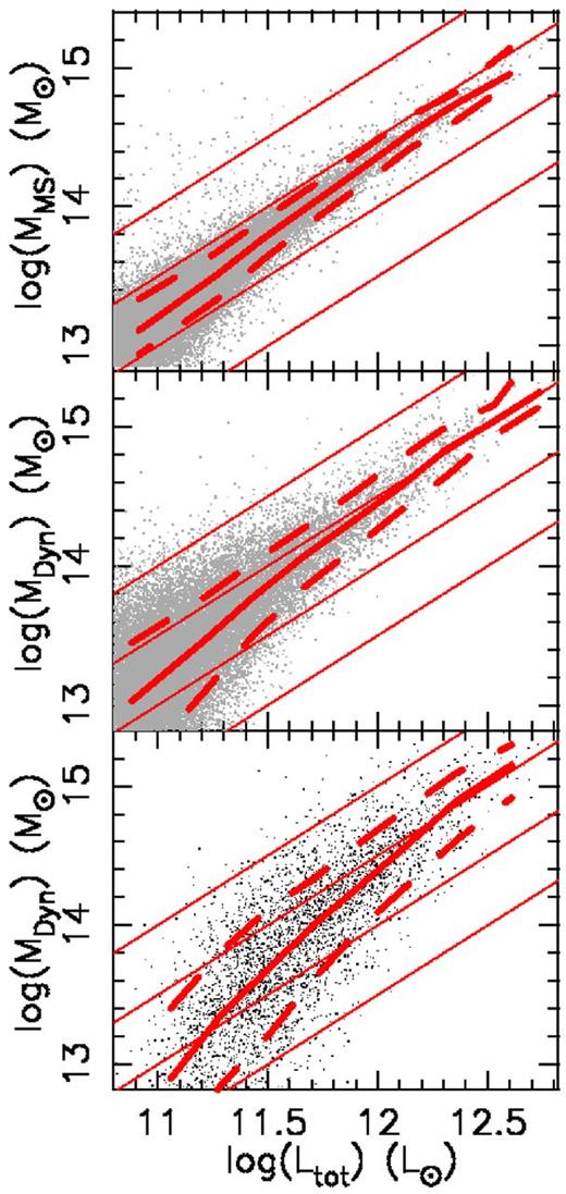
The r band mass–luminosity relation of groups/clusters in the MS. In the top panel, MS mass (rather than dynamical mass) is plotted, while the bottom two panels show dynamical mass. In the top two panels, all systems with redshift less than 0.16 are shown, while in the bottom panel our observational selection criterion of a minimum of six bright galaxies within R200 of systems at 0.05 < z < 0.16 is applied. Solid and dashed red lines are the median with 15th and 85th percentiles, respectively.
Comparing first the top two panels, the displacement and non-linearity in the relation between MS mass and dynamical mass identified in Fig. 2 is also evident when comparing these two plots. A marked increase in scatter is also clearly seen in the dynamical mass data.
Comparison of the bottom two panels shows that the effect of requiring six or more bright members (r < 17.7 mag) within R200 and restricting the redshift range to 0.05 < z < 0.16. Clearly, at low masses, when combined with the requirement of a minimum number of bright members for dynamical analysis, this redshift restriction causes only the brightest groups and clusters at any given mass to be selected, thus introducing another strong non-linearity into the apparent mass–luminosity relation. What is more, comparison of the bottom plot with the r band data in Fig. 3 suggests that the MS is reproducing the observational data extremely well.
In order to demonstrate this, in Fig. 5, we plot the predictions of the simulation for the mass-to-light ratio against mass scaling relation and compare to the medians of the observational data and their uncertainties. We choose to show mass-to-light ratio here as the relatively small dynamical range of this parameter serves to emphasize similarities and differences between the various data sets, while the binning of the data has significantly reduced the correlated errors which would otherwise make interpretation of such a plot difficult.
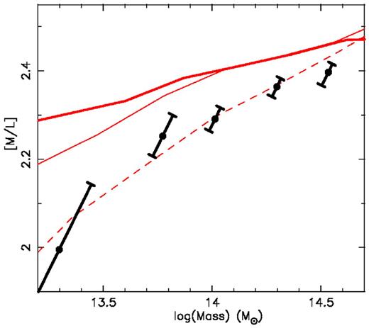
Mass-to-light ratio in the r band is plotted against mass. The medians of observational data and their (correlated) uncertainties are shown as black points with error bars. MS data are shown as red lines. Data taken directly from the MS are shown a thick solid line, while the data for dynamical masses derived from the simulation with no selection criteria applied (see text) are shown a thin red line. The data from the simulation using dynamical mass and with selection criteria applied is shown as a dashed line. The simulation clearly reproduces the observational data extremely well.
In Fig. 5, the data taken directly from the MS is shown as a thick solid line. For ease of comparison, this line has been shifted by the ∼0.1 dex offset between MS and dynamical masses first identified in Fig. 2 and also evident in Fig. 4. The data for dynamical masses with no luminosity or redshift selection criteria applied is shown as a thin solid line, while the dynamical mass data with luminosity and redshift selection criteria applied are shown as a dashed line.
The changing slope in the MS mass against dynamical masses relation noted in Fig. 2 at ∼1014 M⊙ is again evident in this plot, with the two solid lines exhibiting the same shallow slope above this mass, but steepening and diverging below. Examination of Fig. 5 also shows that the MS prediction for the locus of mass-to-light ratio against mass relation for data using dynamical masses and with selection criteria applied (dashed line) is an extremely good match to the observational data. What is more, in Table 2, we show the width of the 15th and 85th percentiles in dynamical mass at selected points along the mass–luminosity relations of the simulated and real data, and agreement is again excellent. Clearly, the MS is doing a remarkably good job of reproducing the actual observational data.
The offsets from the median of the 15th and 85th percentiles in three masses bins in both our data and the MS.
| Data | MS | |||
|---|---|---|---|---|
| log(M) (M⊙) | 15 per cent | 85 per cent | 15 per cent | 85 per cent |
| 13.3 | −0.52 | 0.39 | −0.50 | 0.45 |
| 14.0 | −0.32 | 0.30 | −0.39 | 0.33 |
| 14.7 | −0.27 | 0.27 | −0.28 | 0.25 |
| Data | MS | |||
|---|---|---|---|---|
| log(M) (M⊙) | 15 per cent | 85 per cent | 15 per cent | 85 per cent |
| 13.3 | −0.52 | 0.39 | −0.50 | 0.45 |
| 14.0 | −0.32 | 0.30 | −0.39 | 0.33 |
| 14.7 | −0.27 | 0.27 | −0.28 | 0.25 |
Our analysis of the MS has therefore clearly identified the importance of selection effects in shaping the locus of the mass–luminosity relation found from our data, and suggests that such effects may be present to, some lesser extent, in the other studies considered here. Indeed, the excellent agreement found between our data and the MS suggest that the simulation might be used to identify, and even correct for, such effects in future studies.
4 CONCLUSIONS
As the first step in a program to perform a detailed study of ‘fossil groups’, we have estimated masses and total luminosities in ∼600 groups and clusters identified in the maxBCG catalogue using SDSS photometry and spectroscopy. We have also performed an analysis of MS data subjected to the same processes and selection criteria as the observational data. We have compared our results with five other studies in the literature in four different wavebands (B, r, i and K) and the MS data.
At high masses (>1014 M⊙), we find extremely good agreement with four of the five literature and the MS results, but find an exception in a single literature study (Girardi et al. 2002), which appears discordant. At lower masses the agreement of our data with literature results is poorer. However, we have used the MS to demonstrate that a large part of the discrepancies at these masses can be explained by selection effects.
We have also used the MS to provide a hint to the cause of remaining discrepancies at lower mass, showing that within the simulation the assumption that mass is proportional to σ3 begins to fail as one approaches lower masses. With hints of a similar phenomena already having been observed in X-ray data (e.g. Helsdon & Ponman 2000; Osmond & Ponman 2004), this is an issue that certainly warrants further investigation. It should be noted that our findings with regard the MS are of particular importance in studies that attempt to measure the gradient of the mass-to-light ratio against mass scaling relation which, as is evident from our results, are extremely susceptible to these effects.
The authors would like to thank Eduardo Cypriano for many useful discussions. RP acknowledges the support of CNPq (through PCI-DA grant 301253/2013-7 associated with the PCI/MCT/ON program) CMdO acknowledges support from FAPESP (grant no. 2006/56213-9) and CNPq. LA acknowledges support from a CNPq PIBIC fellowship. The MS data bases used in this paper and the web application providing online access to them were constructed as part of the activities of the German Astrophysical Virtual Observatory. Funding for SDSS-III has been provided by the Alfred P. Sloan Foundation, the Participating Institutions, the National Science Foundation and the US Department of Energy Office of Science. The SDSS-III web site is http://www.sdss3.org/. SDSS-III is managed by the Astrophysical Research Consortium for the Participating Institutions of the SDSS-III Collaboration including the University of Arizona, the Brazilian Participation Group, Brookhaven National Laboratory, Carnegie Mellon University, University of Florida, the French Participation Group, the German Participation Group, Harvard University, the Instituto de Astrofisica de Canarias, the Michigan State/Notre Dame/JINA Participation Group, Johns Hopkins University, Lawrence Berkeley National Laboratory, Max Planck Institute for Astrophysics, Max Planck Institute for Extraterrestrial Physics, New Mexico State University, New York University, Ohio State University, Pennsylvania State University, University of Portsmouth, Princeton University, the Spanish Participation Group, University of Tokyo, University of Utah, Vanderbilt University, University of Virginia, University of Washington and Yale University.
N.B. We have converted the bj given in Eke et al. (2004b) to the B band using the relation Lbj = 1.1LB given by their equation (4.3).
REFERENCES
SUPPORTING INFORMATION
Additional Supporting Information may be found in the online version of this article:
Table 1. An example of the data published online.
Please note: Oxford University Press are not responsible for the content or functionality of any supporting materials supplied by the authors. Any queries (other than missing material) should be directed to the corresponding author for the article.
