


Abstract
Observations of the magnetic fields of young solar-type stars provide a way to investigate the signatures of their magnetic activity and dynamos. Spectropolarimetry enables the study of these stellar magnetic fields and was thus employed at the Télescope Bernard Lyot and the Anglo-Australian Telescope to investigate two moderately rotating young Sun-like stars, namely HD 35296 (V119 Tau, HIP 25278) and HD 29615 (HIP 21632). The results indicate that both stars display rotational variation in chromospheric indices consistent with their spot activity, with variations indicating a probable long-term cyclic period for HD 35296. Additionally, both stars have complex, and evolving, large-scale surface magnetic fields with a significant toroidal component. High levels of surface differential rotation were measured for both stars. For the F8V star HD 35296 a rotational shear of ΔΩ = 0.22|$^{+0.04}_{-0.02}$| rad d− 1 was derived from the observed magnetic profiles. For the G3V star HD 29615, the magnetic features indicate a rotational shear of ΔΩ = 0.48|$_{-0.12}^{+0.11}$| rad d− 1, while the spot features, with a distinctive polar spot, provide a much lower value of ΔΩ of 0.07|$_{-0.03}^{+0.10}$| rad d− 1. Such a significant discrepancy in shear values between spot and magnetic features for HD 29615 is an extreme example of the variation observed for other lower mass stars. From the extensive and persistent azimuthal field observed for both targets, it is concluded that a distributed dynamo operates in these moderately rotating Sun-like stars, in marked contrast to the Sun's interface-layer dynamo.
1 INTRODUCTION
Observations of the distribution of magnetic fields offer insights into how magnetic dynamos are governed by physical properties such as mass, rotation and age, with younger Sun-like stars providing proxies for understanding the history of the Sun's activity and dynamo. Today we can readily observe the starspots and surface magnetic fields of young Sun-like stars, to reconstruct their surface magnetic topologies and differential rotation. Multi-epoch observations of stellar magnetic regions also offer the prospect of revealing how magnetic activity cycles can emerge in stars like the Sun. Such observations can allow us to study the relative role of two possible dynamo theories, namely the widely accepted Sun's ‘shell’ dynamo that operates at the interface layer between the radiation and convection zone and the ‘distributed’ dynamo thought to be operating in young, active stars where the dynamo is present throughout the convection zone (e.g. Brandenburg et al. 1989; Moss et al. 1995; Donati et al. 2003a; Brown et al. 2010). While the large-scale toroidal magnetic field is understood to be buried deep inside the Sun, it has been observed on a range of rapidly rotating solar-type stars through the presence of strong unipolar surface azimuthal magnetic fields (e.g. Donati et al. 2003a; Petit et al. 2004a; Marsden et al. 2006). Petit et al. (2008) concluded that the rotation period threshold where the surface toroidal field begins to dominate over the poloidal field is ≈12 d. Thus, rotation plays an important role in the generation of the magnetic field and the complexity of these fields.
The study of these complex magnetic fields on Sun-like stars has been greatly advanced using the technique of Zeeman–Doppler imaging (ZDI; Semel 1989; Donati & Semel 1990; Donati & Brown 1997; Donati et al. 2003a). ZDI has been performed for a small sample of single, rapidly rotating early G-type stars such as HD 171488 (V889 Her; SpType: G2V; Marsden et al. 2006; Jeffers & Donati 2008; Jeffers et al. 2011) and HD 141943 (SpType: G2; Marsden et al. 2011a,b). Differential rotation, given its likely importance to the operation of the dynamo, is a key measurement. These stars have shown significant levels of differential rotation using both brightness and magnetic features. Jeffers & Donati (2008) observed HD 171488 and measured ΔΩ = 0.52 ± 0.04 rad d− 1 using spot features while ΔΩ = 0.47 ± 0.04 rad d− 1 was measured using magnetic features. Jeffers et al. (2011) in their more recent study measured slightly lower values of ΔΩ ∼ 0.4 rad d− 1 (Stokes I) and ∼0.415–0.45 rad d− 1 (Stokes V). These levels of differential rotation are similar to an earlier study by Marsden et al. (2006) of ΔΩ = 0.402 ± 0.044 rad d− 1 (using spot features). Marsden et al. (2011b) observed HD 141943 and measured ΔΩ = 0.24 ± 0.03 rad d− 1 using spot features with ΔΩ = 0.45 ± 0.08 rad d− 1 using magnetic features on their 2010 data set (and slightly lower with ΔΩ = 0.36 ± 0.09 rad d− 1 for their 2007 data). Conversely, slowly rotating stars such as HD 190771 (SpType: G2V), with a vsin i of 4.3 ± 0.5 km s−1, also exhibit measurable differential rotation with ΔΩ = 0.12 ± 0.03 rad d− 1 using magnetic features (Petit et al. 2008). In addition to relatively high levels of differential rotation, all three stars exhibited complex magnetic topologies with large-scale poloidal and toroidal fields, each with significant higher order components beyond simple dipole fields.
Barnes et al. (2005) first reported the link between differential rotation and effective temperature, and consequently convective turnover time. They were able to develop a correlation between rotational shear and effective temperature for a small sample of stars and determined that as a star's effective temperature increases so does the rotational shear, a trend consistent with the recent theoretical calculations by Kitchatinov & Olemskoy (2011). Additionally, a steep rise in differential rotation for late F-/early G-type stars appears related to the rapid shallowing of the convection zone (e.g. Marsden et al. 2011b). Küker, Rüdiger & Kitchatinov (2011) demonstrate that the extreme levels of rotational shear observed for stars such as HD 171488 can only be explained with a shallow convection zone. Thus, the depth of the convection zone must have a major role in the rotational profile of a solar-type star.
In this study, two moderately rotating, young Sun-like stars were selected based on their similar rotational velocities and sizes, enabling comparisons of their magnetic fields and differential rotations. HD 35296 (SpType: F8V) is a |$1.06_{-0.05}^{+0.06}$| M⊙ (Holmberg, Nordström & Anderson 2009) star with an estimated photospheric temperature 6170 K (Casagrande et al. 2011) while HD 29615 (SpType: G3V) is a 0.95 M⊙, 1.0 R⊙ star (Allende Prieto & Lambert 1999). HD 35296 has a vsin i of 15.9 km s−1 (Ammler-von Eiff & Reiners 2012) while HD 29615 has a vsin i of ∼18 km s−1 (Waite et al. 2011a). The aim is to map the surfaces of these two stars with a view to measuring the rotational shear and magnetic field structures. This will enable further comparisons with stars of similar mass but different rotational velocities. This is Paper I of two papers focusing on the complex nature of the magnetic field topologies of young moderately rotating Sun-like stars as proxies for the evolution of the young Sun. Paper II will focus on the infant Sun EK Draconis (Waite et al., in preparation). This paper is part of the BCool1 collaboration investigating the magnetic activity of low-mass stars (e.g. Marsden et al. 2014).
2 FUNDAMENTAL PARAMETERS OF THE STARS
The fundamental parameters for the two targets, HD 35296 and HD 29615, are shown in Table 1. Some of these parameters such as projected rotational velocity (vsin i), radial velocity and inclination were measured as part of the imaging process, as explained in Section 5, while other parameters have been taken from the literature.
The parameters used to produce the maximum-entropy image reconstructions of the two targets, including surface differential rotation measurements. Except otherwise indicated, parameters have been determined by this study.
| Parameter | HD 35296 | HD 29615 |
|---|---|---|
| Spectral type | F8V1 | G3V2 |
| Equatorial period | 3.48 ± 0.01 d 3 | 2.34|$_{-0.05}^{+0.02}$| d 4 |
| Inclination angle | 65° ± 5°5 | |$65_{-10}^{+5} {}^{\circ}$| |
| Projected rotational velocity, vsin i | 15.9 ± 0.1 km s−1 | 19.5 ± 0.1 km s−1 |
| Photospheric temperature, Tphot | 6170 K 6 | 5820 ± 50 K 7 |
| Spot temperature, Tspot | – | 3920 K 8 |
| Radial velocity, vrad | 38.1 ± 0.1 km s−1 | 19.33 ± 0.1 km s−1 |
| Stellar radius | 1.10 R|$_{{\odot }}^{9}$| | 1.0 |$\mathrm{R}_{\odot }^{10}$| |
| Stellar mass | |$1.06_{-0.05}^{+0.06} \mathrm{M}_{\odot }^{9}$| | 0.95 |$\mathrm{M}_{\odot }^{10}$| |
| Age | 30–50 Myr 11 | 30 Myr12 |
| Convection zone depth11R⋆(R⊙) | 0.178 (0.201) | 0.252 (0.252) |
| Stokes I: Ωeqrad d− 1 | – | 2.68|$_{-0.02}^{+0.06}$| |
| Stokes I: ΔΩrad d− 1 | – | 0.07|$_{-0.03}^{+0.10}$| |
| Stokes V: Ωeqrad d− 1 | 1.804 ± 0.005 | 2.74|$_{-0.04}^{+0.02}$| |
| Stokes V: ΔΩrad d− 1 | 0.22|$^{+0.04}_{-0.02}$| | 0.48|$_{-0.12}^{+0.11}$| |
| Epoch of zero phase (MHJD)13 | 54133.871035 (2007) | 55165.011060 (2009) |
| 54496.094272 (2008) |
Notes.1Montes et al. (2001).
2Torres et al. (2006).
3Using Stokes V data.
4Using Stokes I data.
5The inclination angle of HD 35296 was based on the most recent value of P sinθ = 3.9 calculated by Ammler-von Eiff & Reiners (2012).
6Casagrande et al. (2011).
7Using the bolometric corrections of Bessell et al. (1998).
8Using the relationship between photospheric and spot temperature provided by Berdyugina (2005).
9Based on the values found in Holmberg et al. (2009).
10Allende Prieto & Lambert (1999).
11Determined from the stellar evolution models of Siess et al. (2000).
12Zuckerman & Song (2004).
13Modified Heliocentric Julian Date (MHJD) = HJD − 24000000.0.
2.1 HD 35296
HD 35296 (V1119 Tau) is an F8V star (Montes et al. 2001). It has a parallax of 69.51 ± 0.38 mas (van Leeuwen 2007) giving a distance of 14.39 ± 0.08 pc. Samus et al. (2009) identified HD 35296 as a BY Draconis-type variable star. The range of age estimates of this star in the literature is quite large, with Holmberg et al. (2009) estimating an age of 3.3 Gyr, with some authors listing this star as young as 20 Myr or as old as 7.5 Gyr (e.g. Barry 1988; Chen et al. 2001). The equivalent width of the Li i 670.78 nm line is 99 mÅ, correcting for the nearby 670.744 nm Fe i line using the same factor developed by Soderblom et al. (1993a,b). This is consistent with that measured by Takeda & Kawanomoto (2005) of 94.3 mÅ. Li & Hu (1998) argued that HD 35296 is a member of the Taurus-Auriga star-forming region that may have reached the zero-age main sequence. When placing this star on the theoretical isochrones of Siess, Dufour & Forestini (2000), the age of this star is between 20 and 50 Myr. Hence, it is likely that this star is quite youthful.
2.2 HD 29615
HD 29615 (HIP 21632) is a G3V star (Torres et al. 2006). The Hipparcos space mission measured a parallax of 18.27 ± 1.02 mas (van Leeuwen 2007), giving a distance of |$54.7_{-2.9}^{+3.2}$| pc. Zuckerman & Song (2004) proposed that HD 29615 was a member of the Tucana/Horologium association indicating an age of ∼30 Myr. Waite et al. (2011a) detected a magnetic field on this star, along with a varying emission equivalent width for the Hα line in the range from ∼370 to ∼500 mÅ demonstrating the presence of a very active, and variable, chromosphere.
3 OBSERVATIONS AND ANALYSIS
HD 35296 was observed at the Télescope Bernard Lyot (TBL, Observatoire Pic du Midi, France) in 2007 January/February and again in 2008 January/February using the high-resolution spectropolarimeter NARVAL. HD 29615 was observed at the Anglo-Australian Telescope (AAT, New South Wales, Australia) in 2009 November/December using the high-resolution spectropolarimeter Semel Polarimeter (SEMPOL). Journals of observations are given in Tables 2 and 3.
Journal of spectropolarimetric observations of HD 35296 using the TBL.
| ut date | ut | Exp. time1 | Mean SNR for |
|---|---|---|---|
| middle | (s) | Stokes V | |
| LSD profiles | |||
| 2007 Jan 24 | 21:08:45 | 1 × 300 | –2 |
| 2007 Jan 26 | 21:10:23 | 4 × 300 | 19 762 |
| 2007 Jan 27 | 20:18:17 | 4 × 600 | 39 439 |
| 2007 Jan 29 | 19:29:15 | 4 × 600 | 38 358 |
| 2007 Feb 02 | 21:17:29 | 4 × 300 | 4223 |
| 2007 Feb 03 | 20:15:21 | 4 × 300 | 29 940 |
| 2007 Feb 04 | 20:06:35 | 4 × 300 | 25 137 |
| 2007 Feb 08 | 20:30:51 | 4 × 300 | 25 639 |
| 2008 Jan 19 | 20:01:46 | 4 × 300 | 17 208 |
| 2008 Jan 20 | 21:45: 1 | 4 × 300 | 20 581 |
| 2008 Jan 21 | 19:42:27 | 4 × 300 | 24 563 |
| 2008 Jan 21 | 20:53:24 | 4 × 200 | 22 146 |
| 2008 Jan 22 | 20:09:11 | 4 × 300 | 21 913 |
| 2008 Jan 23 | 20:10:31 | 4 × 300 | 21 825 |
| 2008 Jan 24 | 20:39:32 | 4 × 300 | 13 296 |
| 2008 Jan 25 | 20:15:17 | 4 × 300 | 19 723 |
| 2008 Jan 26 | 20:14:43 | 4 × 300 | 21 148 |
| 2008 Jan 27 | 20:30:50 | 4 × 300 | 21 245 |
| 2008 Jan 28 | 21:56:43 | 4 × 300 | 21 245 |
| 2008 Jan 29 | 20:50:19 | 4 × 300 | 25 946 |
| 2008 Feb 02 | 20:45:15 | 4 × 300 | 24 375 |
| 2008 Feb 04 | 20:20:19 | 4 × 300 | 27 669 |
| 2008 Feb 05 | 20:21:18 | 4 × 300 | 22 909 |
| 2008 Feb 06 | 21:11: 7 | 4 × 300 | 25 579 |
| 2008 Feb 09 | 20:34:17 | 4 × 300 | 24 555 |
| 2008 Feb 10 | 19:13:58 | 4 × 300 | 29 354 |
| 2008 Feb 11 | 20:39:11 | 4 × 300 | 25 414 |
| 2008 Feb 12 | 20:45:32 | 4 × 300 | 27 269 |
| 2008 Feb 13 | 20:39:30 | 4 × 300 | 24 182 |
| 2008 Feb 14 | 21:00: 8 | 4 × 300 | 24 386 |
| 2008 Feb 15 | 20:37: 6 | 4 × 300 | 28 120 |
Notes.1Each sequence consists of four sub-exposures with each sub-exposure being 300 s (for example).
2Only one Stokes I spectrum was taken on this night. The SNR, as measured for order number 41, was 272.
Journal of spectropolarimetric observations of HD 29615 using the AAT.
| ut date | ut | Exp. time1 | Mean SNR for |
|---|---|---|---|
| middle | (s) | Stokes V | |
| LSD profiles | |||
| 2009 Nov 25 | 11:03:28 | 4 × 750 | 5567 |
| 2009 Nov 25 | 13:04:01 | 4 × 750 | 6337 |
| 2009 Nov 25 | 16:29:33 | 4 × 750 | 4908 |
| 2009 Nov 27 | 10:23:36 | 4 × 750 | 6171 |
| 2009 Nov 27 | 13:28:05 | 4 × 750 | 6978 |
| 2009 Nov 27 | 16:28:02 | 4 × 750 | 5610 |
| 2009 Nov 28 | 10:10:47 | 4 × 750 | 3821 |
| 2009 Nov 28 | 13:13:08 | 4 × 750 | 5971 |
| 2009 Nov 28 | 16:15:29 | 4 × 750 | 4280 |
| 2009 Nov 29 | 10:08:37 | 400 + 3 × 750 | 5785 |
| 2009 Nov 29 | 13:23:08 | 4 × 750 | 4604 |
| 2009 Nov 29 | 16:23:23 | 4 × 750 | 3493 |
| 2009 Nov 30 | 11:05:48 | 4 × 750 | 3283 |
| 2009 Nov 30 | 16:18:04 | 4 × 750 | 3713 |
| 2009 Dec 01 | 11:02:55 | 4 × 750 | 6353 |
| 2009 Dec 01 | 14:13:39 | 4 × 750 | 4961 |
| 2009 Dec 02 | 10:36:24 | 4 × 750 | 6158 |
| 2009 Dec 02 | 13:04:01 | 4 × 750 | 6176 |
| 2009 Dec 02 | 16:03:39 | 4 × 750 | 4651 |
| 2009 Dec 03 | 10:27:35 | 4 × 750 | 4228 |
| 2009 Dec 03 | 13:33:32 | 4 × 750 | 6312 |
Note.1Each sequence consists of four sub-exposures with each sub-exposure being 750 s (for example).
3.1 High-resolution spectropolarimetric observations from the TBL
NARVAL is a bench-mounted, cross-dispersed échelle spectrograph, fibre-fed from a Cassegrain-mounted polarimeter unit and is similar in function to the SEMPOL used at the AAT, which is described in Section 3.2. NARVAL has a mean pixel resolution of 1.8 km s−1 pixel−1 with a spectral coverage from ∼370 to 1048 nm with a resolution of ∼65 000 spanning 40 grating orders (orders #22 to #61). NARVAL consists of one fixed quarter-wave retarder sandwiched between two rotating half-wave retarders and coupled to a Wollaston beamsplitter (Aurière 2003). Observations in circular polarization (Stokes V) consist of a sequence of four exposures. After each of the exposures, the half-wave Fresnel rhomb of the polarimeter is rotated so as to remove any systematic effects due to variations in the optical throughput, CCD inhomogeneities, terrestrial and stellar rotation, temporal variability and instrumental polarization signals from the telescope and the polarimeter (e.g. Semel, Donati & Rees 1993; Carter et al. 1996; Donati et al. 2003a). Initial reduction was completed using the dedicated pipeline reduction software libre-esprit (Échelle Spectra Reduction: an Interactive Tool), which is based on the algorithm developed by Donati et al. (1997). Silvester et al. (2012) proved that NARVAL is a very stable instrument, with resolution and signal-to-noise ratio (SNR) being constant over the four years of data studies from 2006 to 2010.
3.2 High-resolution spectropolarimetric observations from the AAT
High-resolution spectropolarimetric data were obtained from the AAT using the University College of London Échelle Spectrograph (UCLES) and SEMPOL (Semel et al. 1993; Donati et al. 1997, 2003a). The detector used was the deep depletion EEV2 CCD with 2048 × 4096 13.5 μm pixel2. UCLES was used with a 31.6 gr/mm grating covering 46 orders (orders # 84 to # 129). The central wavelength was 522.002 nm with full wavelength coverage from 438 to 681 nm. The dispersion of ∼0.004 958 nm at order # 129 gave a resolution of approximately 71 000. The mean resolution for the AAT spectra was determined to be 1.689 km s−1 pixel−1. The operation of SEMPOL is similar to that explained in Section 3.1. After each exposure, the half-wave Fresnel rhomb is rotated between +45° and −45° so as to remove any systematic effects. Initial reduction was completed using esprit developed for SEMPOL (Donati et al. 1997). SEMPOL is not as efficient as NARVAL; hence, the SNR is lower, even though the AAT is a 3.9 m telescope whereas the TBL is a 2 m telescope. In addition, the spectral range of SEMPOL is smaller; therefore, there are fewer spectral lines available to extract the magnetic signature from the star's light.
3.3 Spectropolarimetric analysis
Preliminary processing involved subtracting the bias level and using a nightly master flat combining typically 20 flat-field exposures. Each stellar spectrum was extracted and wavelength calibrated against a thorium–argon lamp.
After using libre-esprit (TBL) or esprit (AAT), the technique of least-squares deconvolution (LSD) was applied to the reduced spectra. LSD combines the information from many spectral lines to produce a single line profile, thereby providing an enormous multiplex gain in the SNR (e.g. Donati & Collier-Cameron 1997; Donati et al. 1997; Kochukhov, Makaganiuk & Piskunov 2010). A G2 line mask created from the Kurucz atomic data base and ATLAS9 atmospheric models (Kurucz 1993) was used to compute the average line profile for both stars. Tables 2 and 3 lists the SNR for each individual Stokes V LSD profile.
In order to correct for the minor instrumental shifts in wavelength space due to atmospheric temperature or pressure fluctuations, each spectrum was shifted to match the centroid of the Stokes I LSD profile of the telluric lines contained in the spectra, as was performed by Donati et al. (2003a) and Marsden et al. (2006). Further information on LSD can be found in Donati et al. (1997) and Kochuknov et al. (2010).
4 CHROMOSPHERIC ACTIVITY INDICATORS
Chromospheric activity can be determined using the Ca ii H&K, Ca ii infrared triplet (IRT) and Hα spectral lines. The two Ca ii H&K absorption lines are the most widely used optical indicators of chromospheric activity. There have been a number of long-term monitoring studies of the variation of Ca ii H&K in solar-type stars spanning several decades. One study is the Mount Wilson Ca H&K project (e.g. Wilson 1978; Duncan et al. 1991). From this survey, differential rotation and solar-like activity cycles have been inferred on a number of solar-type stars (e.g. Baliunas et al. 1985; Donahue & Baliunas 1992; Donahue 1993; Donahue & Baliunas 1994).
The source functions of the Ca ii H&K lines are collisionally controlled and hence are very sensitive to electron density and temperature. The Ca ii IRT lines share the upper levels of the H&K transitions and are formed in the lower chromosphere (e.g. Montes et al. 2004). The Hα spectral line is also collisionally filled in as a result of the higher temperatures and is formed in the middle of the chromosphere and is often associated with plages and prominences (e.g. Thatcher & Robinson 1993; Montes et al. 2004).
The Ca ii H&K and Ca ii IRT spectral lines were observed for HD 35296 but not for HD 29615 as the spectral range of SEMPOL does not extend far enough into the respective regions to permit monitoring of these diagnostic lines.
4.1 TBL activity indices for HD 35296
Morgenthaler et al. (2012) previously reported that the spectra in the region of the Ca ii H&K are not well normalized by the pipeline reduction due to the dense distribution of photospheric lines. However, we did not adopt their method as a number of tests showed that simply removing the overlapping section of the order provided commensurate results as renormalizing the spectra.
Fig. 1 shows the variation in the Ca ii H&K lines, Ca ii IRT and Hα spectral lines during 2007 (left-hand panels) and 2008 (right-hand panels) for HD 35296. The epoch for the 2007 data was set to the middle of the observation run whereas the epoch of the 2008 data was set to 104 stellar rotations later on and was chosen to be close to the middle of the 2008 observation run, as explained in Section 5.2. The index was measured for each spectrum, and then combined in sets of four, coinciding with a cycle of four sub-exposures as explained in Section 3.1. The average of these four indices was determined with the error bar being the minimum and maximum values for that set. The data from 2007 showed limited variation, either due to the reduced coverage or a more homogeneous chromosphere. In contrast, in 2008, HD 35296 exhibited greater modulation of the S-index, Ca IRT index and Hα-index while the average remained very similar with an S-index for 2007 of 0.323 ± 0.008 and for 2008 of 0.322 ± 0.016. This is consistent, within error limits, with the average S-index of 0.308 ± 0.07 from the Mount Wilson survey (Duncan et al. 1991). Using the transformation values from Rutten (1984), log R′HK was determined to be −4.45 ± 0.03. This was an average value of the S-index over the observing runs with the error based on the minimum and maximum values. Table 4 shows the average S-index, NHα and NCaIRT indices for 2007 and 2008. Each value is the average over the observing run with the error showing the variation during this time, most likely as a result of modulation due to the rotation of the star.
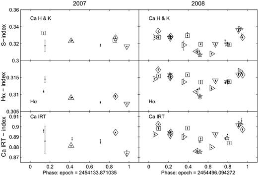
The variation in the Ca ii H&K lines (upper), Hα (middle) and Ca ii IRT (lower) spectral lines during 2007 (left) and 2008 (right) for HD 35296. The index was measured for each spectrum, and then combined in sets of four, coinciding with a cycle of four sub-exposures as explained in Section 3.1. The average of these four indices was determined with the error bar being the minimum and maximum values for that set. The rotational period used was 3.48 d. The observing run covered ∼4.3 rotations in 2007 and ∼7.7 rotations in 2008. The symbols represent the respective rotations: ‘.’ only = first, ‘⋄’ = second, ‘□’ = third, ‘▵’ = fourth, ‘▿’ = fifth, ‘⊲’ = sixth, ‘⊳’ = seventh and ‘☆’ = eighth rotation.
HD 35296: average activity indices using the Ca ii H&K, Hα and Ca ii IRT spectral lines. The error estimate is based on the range of values during each observing run.
| Index | 2007 | 2008 |
|---|---|---|
| S-index1 | 0.323 ± 0.008 | 0.322 ± 0.016 |
| NHα | 0.310 ± 0.004 | 0.314 ± 0.004 |
| NCaIRT | 0.887 ± 0.011 | 0.891 ± 0.015 |
| Index | 2007 | 2008 |
|---|---|---|
| S-index1 | 0.323 ± 0.008 | 0.322 ± 0.016 |
| NHα | 0.310 ± 0.004 | 0.314 ± 0.004 |
| NCaIRT | 0.887 ± 0.011 | 0.891 ± 0.015 |
4.2 AAT Hα activity index for HD 29615
The Hα spectral line was used as a chromospheric indicator for HD 29615. A similar approach, as explained in Section 4.1, was applied to the AAT data. The overlapping sections of the AAT spectra were removed and the continuum checked against a synthetic spectrum obtained from the POLLUX data base. In all cases, the continuum near the Hα spectral line closely matched the synthetic spectra. Equation (2) was then used to determine the Hα-index for HD 29615. Fig. 2 shows how this Hα-index varied over the rotation period of HD 29615. The error bars indicate the range of the measurement during a cycle of four sub-exposures, as explained in Section 3.1. This supports the variable nature of the mid-level chromosphere, first observed by Waite et al. (2011a).
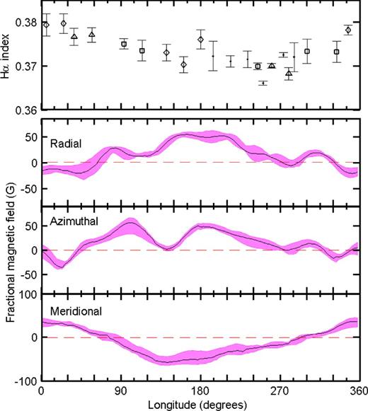
The top panel represents the variation in the Hα-index as a function of longitude for HD 29615 (see Section 4.2). The observing run covered ∼3.5 rotations. The symbols represent the respective rotations: ‘.’ = first, ‘⋄’ = second, ‘□’ = third and ‘▵’ = fourth rotation. The bottom three panels represent the variation in magnetic field strength for each configuration as a function of longitude (see Section 6.1). The shaded regions show the variation in the strength at each longitude as determined by varying vsin i, inclination angle, Ωeq and ΔΩ within the limits of their respective accuracy. The epoch was set to MHJD = 55165.011060 with a rotational period of 2.34 d.
5 IMAGE RECONSTRUCTION
Surface images of these moderately rotating stars were generated through the inversion of a time series of LSD profiles of Stokes I (brightness images) or Stokes V (magnetic images). The ZDI code used was that of Brown et al. (1991) and Donati & Brown (1997). Because this inversion process is an ill-posed problem where an infinite number of solutions are possible when fitting to the noise level, this code implements the Skilling & Bryan (1984) maximum-entropy optimization that produces an image with the minimum amount of information required to fit the data to the noise level.
5.1 Brightness image of HD 29615
Brightness images were not reconstructed for HD 35296 as the vsin i of 15.9 km s−1 is below the usual limit for Doppler imaging (DI). In contrast, the observed intensity profiles for HD 29615 contained sufficient information for both mapping and a measurement of differential rotation using spot features.
A two-temperature model, one being the temperature of the quiet photosphere while the second is that of the cool spots, has been used to reconstruct the brightness image for HD 29615. Synthetic Gaussian profiles were used to represent the profiles of both the spot and photosphere. Unruh & Collier Cameron (1995) showed that the use of these synthetic profiles provides brightness maps that are very similar to those maps created by using profiles from slowly rotating stars of commensurate temperature. Hence, many authors now adopt this approach (e.g. Petit et al. 2004b; Marsden et al. 2005, 2006, 2011a,b; Waite et al. 2011b). Using the relationship between photospheric and spot temperature provided by Berdyugina (2005), the spot temperature of HD 29615 was estimated to be 3920 K.
The imaging code was used to establish the values of a number of basic parameters, including the star's projected rotational velocity, vsin i, and radial velocity, vrad. This was achieved by systematically varying each parameter in order to minimize the reduced-χ2 (|$\chi ^2_{{\rm r}}$|) value (e.g. Marsden et al. 2005; Jeffers & Donati 2008). These key stellar parameters were determined with initially vrad and then vsin i. This sequence was repeated each time additional parameters, such as inclination or differential rotation parameters, were modified as a result of the imaging process.
The inclination angle for HD 29615 was estimated using the bolometric corrections of Bessell, Castelli & Plez (1998) and was confirmed using the imaging code. This value was determined to be 65|$^{+5}_{10}$|°. The minimum angle of ∼50° assumed a stellar radius of 1.2 R⊙ (Messina et al. 2010). A linear limb-darkening coefficient of 0.62 was used (Sing 2010). The full set of parameters that gave the minimum |$\chi ^2_r$| value of 0.45 are shown in Table 1 and were adopted when producing the final DI map as shown in the top-left panel of Fig. 3. A |$\chi ^2_{{\rm r}}$| value less than 1 is possible as the SNR calculated for the LSD Stokes I profiles are underestimated (e.g. Petit et al. 2004b; Marsden et al. 2011a). Nevertheless, this has no impact on the final brightness maps. The maximum-entropy fits to the Stokes I LSD profiles for HD 29615 with the measured surface differential rotation incorporated into the analysis are shown in Fig. 4. Deviations of the model profile from the observed profile are shown in the dynamic spectrum displayed in Fig. 5. To produce this dynamic spectrum, each observed LSD profile was normalized, and then subtracted from the associated normalized model profile with the residual profile being plotted as the dynamic spectrum. The scale of this dynamic spectrum is ± 4 × 10⁻³ or ≈ 0.4 per cent of the intensity of the line profile. The small residuals indicate that the majority of the large-scale features can be accurately modelled. However, there is a consistent mismatch between the modelled and original data as evidenced by a brighter band near the red wing of the dynamic spectrum. This indicates that the modelled data have not incorporated information from the wings of the original line profiles. This is advantageous in that modelling of that part of the line profile may have led to spurious banding in the resulting image (Unruh & Collier Cameron 1995).
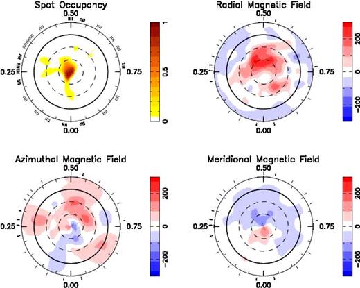
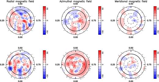
The maximum-entropy brightness and magnetic image reconstructions for HD 29615. These maps are polar projections extending down to −30°. The bold lines denote the equator and the dashed lines are +30° and +60° latitude parallels. The radial ticks indicate the phases at which this star was observed and the scale of the magnetic images is in gauss. Differential rotation, as measured using the Stokes I and V profiles, respectively, has been incorporated into the reconstruction of the maps. The spot map has a spot coverage of 2.6 per cent while the global magnetic field strength is 81.6 G. The epoch was set to MHJD = 55165.011060 with a rotational period of 2.34 d.
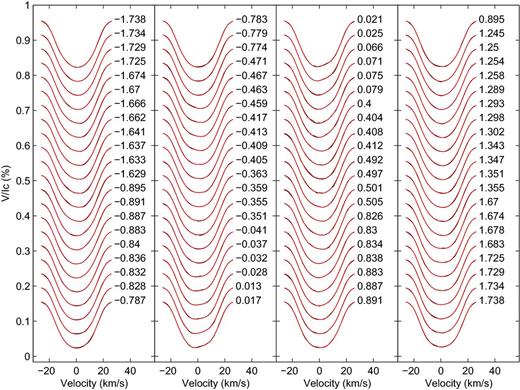
The maximum-entropy fits to the Stokes I LSD profiles for HD 29615 with the measured surface differential rotation incorporated into the analysis. The red lines represent the modelled lines produced by the DI process whereas the black lines represent the actual observed LSD profiles. Each successive profile has been shifted down by 0.020 for graphical purposes. The rotational cycle at which the observation took place is indicated to the right of each profile. The epoch was set to MHJD = 55165.011060 with a rotational period of 2.34 d.
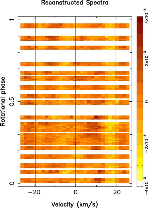
Dynamic spectrum of the residual plot for the Stokes I LSD profiles for HD 29615. Each LSD profile was normalized and subtracted from the associated normalized model profile.
5.2 Magnetic images
The magnetic topology was determined for both HD 35296 and HD 29615 using ZDI. ZDI requires high-SNR data as the polarization signature is typically less than 0.1 per cent of the total light intensity (Donati et al. 1997). The Stokes V data were used to reconstruct radial, azimuthal and meridional fields coinciding with the three vector fields in spherical geometry. The modelling strategy of Donati & Brown (1997) was used to construct the magnetic field topology on both stars. ZDI only measures the large-scale magnetic field as the small-scale magnetic fields cannot be recovered as the positive and negative magnetic fields within the resolution element are likely to cancel each other out. The mapping procedure involved uses the spherical harmonic expansions of the surface magnetic field, as implemented by Donati et al. (2006). The maximum spherical harmonic expansion ℓmax = 11 was selected for HD 35296 while ℓmax = 14 was used for HD 29615. These were the minimum values where any further increase did not produce any difference in the magnitude and topology of the magnetic field recovered.
The magnetic maps for HD 29615 are shown in Fig. 3 while the associated fits between the modelled data and the actual LSD profiles are shown in Fig. 6. The |$\chi ^2_{{\rm r}}$| value of the magnetic models for HD 29615 was 1.25, showing that the fit accuracy was very close to reaching the noise level of the data.

The maximum-entropy fits to the Stokes V LSD profiles for HD 29615 with the measured surface differential rotation incorporated into the analysis. The black lines represent the observed Zeeman signatures, while the red lines represent the modelled lines. Each successive profile has been shifted down by 0.002 for graphical purposes. The minimum |$\chi ^2_{{\rm r}}$| value was set to 1.25. The rotational phases at which the observations took place are indicated to the right of each profile. The error bars to the left of each profile are ±0.5σ. The epoch was set to MHJD = 55165.011060 with a rotational period of 2.34 d.
The magnetic maps for HD 35296 for the 2007 and 2008 data sets are shown in Fig. 7 with the associated fits between the modelled data and the actual profiles shown in Fig. 8. The LSD profile taken on 2007 February 02 of HD 35296 was excluded from the mapping process due to the relatively poor SNR. Including these data made no difference to the resulting magnetic maps and field configuration but did make a marginal degradation of the total magnetic field strength (by 0.1 G). In each case, the minimum |$\chi ^2_{{\rm r}}$| value of the magnetic models was set to 1.0.
Magnetic imaging of the large-scale field for HD 35296 from both the 2007 (top series) and 2008 (bottom series) observing runs. These maps are polar projections, as explained in Fig. 3. The 2007 global magnetic field was 13.4 G whereas the 2008 field was 17.9 G. The epoch was set to MHJD = 54133.871035 for the 2007 data and MHJD = 54496.094272 for the 2008 data, with a rotational period of 3.48 d.
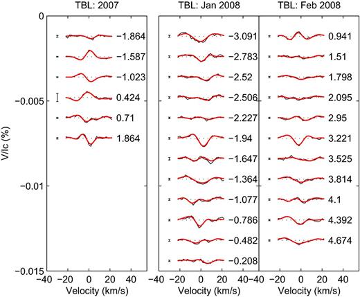
The maximum-entropy fits to the LSD profiles for HD 35296 during 2007 (left-hand panel) and 2008 (right-hand panel), with differential rotation incorporated into the analysis. The observed Zeeman signatures are shown in black while the fit to the data is shown as red lines. The rotational cycle and ±0.5σ error bars of each observation are shown next to each profile. Each profile has been shifted down by 0.0012 for clarity. The minimum |$\chi ^2_{{\rm r}}$| value used was 1.0. The LSD profile obtained on 2007 February 02 was excluded from the mapping process due to its relatively low SNR. The rotational period used was 3.48 d.
The full set of parameters used to produce these maps, including differential rotation (see Section 5.3), are listed in Table 1. Due to the length of time between the observing runs for HD 35296, the phases for the 2007 run were calculated using an epoch of the Modified Heliocentric Julian Date (where MHJD = HJD − 2400000.0) of 54133.871035 whereas the 2008 run used an epoch of MHJD = 54496.094272. This 2008 epoch was selected as it was close to the mid-point of the observing run, but was an integer number of rotations since the mid-point of the 2007 run based on the 3.48 d period.
5.3 Differential rotation
Using the magnetic signatures, HD 35296 has an equatorial rotational velocity, Ωeq, of 1.804 ± 0.005 rad d− 1 with a rotational shear, ΔΩ, of 0.22|$^{+0.04}_{-0.02}$| rad d− 1. Using the brightness features, HD 29615 has an equatorial rotational velocity, Ωeq, of 2.68|$_{-0.02}^{+0.06}$| rad d− 1 with a rotational shear, ΔΩ, of 0.07|$_{-0.03}^{+0.10}$| rad d− 1. Using the magnetic features, HD 29615 has an equatorial rotational velocity, Ωeq, of 2.74|$_{-0.04}^{+0.02}$| rad d− 1 with a rotational shear, ΔΩ, of 0.48|$_{-0.12}^{+0.11}$| rad d− 1 (see Table 1).
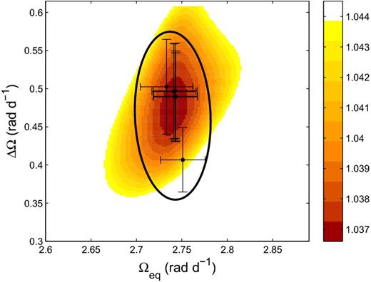
The errors for the differential rotation measurements were calculated by individually varying stellar parameters such as spot occupancy (for Stokes I: ±10 per cent) or global magnetic field (for Stokes V: ±10 per cent), inclination angle (±5° for HD 35296 and +5° and −10° for HD 29615) and vsin i (±0.1 km s−1) and determining the minimum Ωeq–ΔΩ pair from each of the reduced-χ2 landscapes generated. Figs 9 and 10 show the reduced-χ2 landscape for the optimum set of parameters, as listed in Table 1. Superimposed on these are the individual Ωeq–ΔΩ pairs derived from this variation of stellar parameters, with the error bars being 1σ errors in the paraboloid fit. The final ellipse was generated to encompass all the differential rotation values. The true error bars may be slightly larger than this due to intrinsic spot evolution during the data collection (e.g. Morgenthaler et al. 2012). The differential rotation parameters determined for HD 35296 for the 2008 observing run were used in the mapping process for the 2007 data as no differential rotation was able to be determined for this data set due to the limited number of exposures.
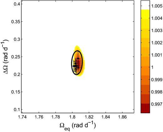
Differential rotation using Stokes V: HD 35296 in 2008. The contour plot is a 1σ projection using the optimum set of parameters, as listed in Table 1. The darker regions correspond to lower reduced-χ2 values. Superimposed on this grid is the error ellipse (thick line) that encompasses a range of Ωeq–ΔΩ pairs determined by varying such parameters as vsin i, magnetic field strength and inclination. Each data point is the result of paraboloid fit of the reduced-χ2 landscape for each individual differential rotation value. The error bars on each data point are 1σ errors in the paraboloid fit.
Differential rotation using Stokes V: HD 29615. The contour plot is a 1σ projection using the optimum set of parameters, as listed in Table 1. Superimposed on this grid is the error ellipse (thick line) encompassing the respective Ωeq–ΔΩ pairs, as explained in Fig. 9. The error bars on each data point are 1σ errors in the paraboloid fit.
6 DISCUSSION
HD 35296 and HD 29615 are two moderately rapidly rotating young Sun-like stars that display rotational variation in their chromospheric activity. In this paper, we have determined the surface topology of both stars revealing complex magnetic fields and high levels of surface differential rotation.
6.1 Chromospheric activity
Chromospheric activity was determined using the Ca ii H&K, Ca ii IRT and Hα spectral lines for HD 35296 while only the Hα line was used for HD 29615 as the spectral range of SEMPOL did not extend far enough into the respective regions to permit monitoring of the Ca ii diagnostic lines. Table 4 shows the average activity indices in 2007 and 2008 for HD 35296. The average S-index was 0.322 ±0.016 while the average Hα-index, NHα, 0.312 ± 0.006 and the average Ca ii IRT index, NCaIRT, was 0.889|$_{-0.013}^{+0.017}$|. Fig. 1 demonstrates the variable nature of the activity of HD 35296. In 2007, the chromosphere was more homogeneous with respect to phase. The large error bar at phase ∼ 0.15 is the result of a poor SNR observation. The amplitude of the modulation in the Ca ii H&K and Hα indices is less than that observed in 2008. This would indicate that HD 35296 is more active during the 2008 epoch. In addition, the error bars on each of the data points do not overlap indicating that the chromosphere not only varied as a function of rotation, but also from one rotation to the next. This is clearly observed in all three chromospheric diagnostic lines. The conclusion is that the chromosphere of HD 35296 is highly variable over a one-month interval of approximately eight stellar rotations.
S-index measurements are also available from Baliunas et al. (1995), where data were obtained between 1966 and 1991. The average S-index from the Baliunas sample is 0.33 ± 0.02 and the log R′HK is −4.36 ± 0.04. Mount Wilson data were not available from 1991 onwards but fortunately Lowell observatory started a long-term Ca ii H&K monitoring programme where HD 35296 was observed from 1994 to 2008 (Hall et al. 2009). All available S-index values scaled to the Mount Wilson system are shown in Fig. 11. HD 35296 exhibits a gradual decrease in its S-index from 1966 to 1980 and shows a relatively flat trend from 1980 onwards. Interestingly, during the low-activity period the S-index does exhibit small variations. The long-term variations also indicate a probable long cyclic period which was also determined by Baliunas et al. (1995). No error estimates are available for the Lowell catalogue.

6.2 Brightness and magnetic maps
The results presented in this paper show that HD 35296 and HD 29615 are young, Sun-like stars whose moderately rapid rotation has led to very complex large-scale surface magnetic field topology. As discussed in Section 5, brightness images were not produced for HD 35296 due to its relatively low vsin i with the LSD intensity profiles not being sufficiently deformed by any surface features present to recover reliable spot information using DI. The brightness map for HD 29615, in Fig. 3 (top-left panel), shows a dominant polar spot. This polar spot is slightly off-centred with features extending to ∼60° latitude for phases between, ϕ, 0.0 and 0.5, but not evident for ϕ = 0.5–1.0. While the polar spot is very prominent, there appears limited spot coverage at mid- to lower latitudes with a small number of features observed at ϕ ∼ 0, 0.25–0.3 and 0.55–0.65. The features at ϕ ∼ 0 and ∼0.25 may not be reliable as the dynamic spectrum shown in Fig. 5 displays a dark diagonal band moving from the blue wing to the red wing. This indicates that the modelled data may have incorporated spots at this phase that were not present in the original data and hence could not accurately constrain the latitude of these two features. Unruh & Collier Cameron (1997) note that spectroscopy extracts the higher latitude features but cannot discriminate lower latitude features at latitudes ≲ 30°. However, the paucity of spots at mid- to lower latitudes is dissimilar to other more rapidly rotating solar-type stars like He 699 (V532 Per, SpType: G2-3V; Jeffers, Barnes & Collier Cameron 2002), HD 106506 (SpType: G1V; Waite et al. 2011b) and HD 141943 (SpType: G2; Marsden et al. 2011a) that appear to have spots covering all latitudes and phases.
The magnetic maps for HD 29615, in Fig. 3, show azimuthal, meridional and radial magnetic field structures. The azimuthal magnetic field is strongly positive although not a complete ring of field, unlike that observed on other solar-type stars such as HD 106506 (Waite et al. 2011b) and HD 141943 (Marsden et al. 2011a). The radial field is also strongly positive at higher latitudes, from approximately +30° to the pole. The maps for HD 35296 from 2007 and 2008 are shown in Fig. 7. Like HD 29615, HD 35296 displays a predominantly positive azimuthal magnetic field in both 2007 and 2008 while the radial and meridional fields show mixed polarity across the surface.
When using Stokes V without Stokes I, Q, U, there is crosstalk between the three magnetic field configurations, although the azimuthal field is the most robust with limited crosstalk. At high latitudes, ZDI can recover all three field components but at lower latitudes, in particular for stars with inclination angles greater than 50°, the crosstalk is from the meridional to radial field component (Donati & Brown 1997). This crosstalk appears stronger for HD 35296 when compared with HD 29615. This could be due to either a weaker magnetic field or fewer phases for each rotation for HD 35296 thereby affecting the code's ability to distinguish between the radial and meridional field components, particularly at lower latitudes. Rosén & Kochukhov (2012) have observed when using all four Stokes IQUV parameters, the crosstalk between the components is significantly reduced. However, the linear polarization states (Stokes Q and U parameters) are significantly weaker than the Stokes V and are extremely difficult to observe on active cool stars such as HD 29615 and HD 35296 (e.g. Wade et al. 2000; Kochukhov et al. 2004).
6.3 Latitude dependence of the magnetic fields
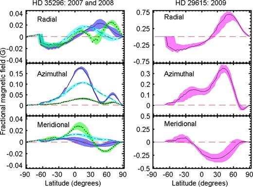
Variation of the respective magnetic field orientations for HD 35296 (left series of panels) and HD 29615 (right series of panels). The shaded regions show the variation in the strength at each latitude point as determined by varying vsin i, inclination angle, Ωeq and ΔΩ within the limits of their respective accuracy (see Section 5.3). Considering HD 35296, the solid line with the dark blue shading is for 2008 data while the dotted line with the green shading is for the 2007 data. The dot–dashed line with cyan shading represents the 2008 data with reduced number of profiles approximately matching the number of profiles and phase of the 2007 data. The period used for HD 35296 was 3.48 d while the period used for HD 29615 was 2.34 d.
To test this, we reduced the number of profiles in the 2008 data set, to match the same number of profiles and phase as that obtained in 2007. This had an impact on the strength of the global magnetic field (17.9 G reduces to 11.9 G) and the latitudinal distribution of the respective fields. The azimuthal field remained strongly positive, as shown in Fig. 12 (dot–dashed line with cyan colour). However, the radial field no longer shows a strong positive peak at ∼70° latitude when compared with using the full number of profiles, although it does remain positive at these mid-latitudes. As a further test, maps were produced from the first two rotations, middle four rotations and final two rotations. This demonstrated the robust nature of the azimuthal magnetic field, although fewer profiles meant that the imaging code could not adequately recover the latitude of each feature. Nevertheless, the mid-latitude reversal in the radial field from 2007 to 2008 may well be real. The evidence is tantalizing but more data would be required before any definitive conclusion can be drawn regarding any changes in the mid-latitude field polarity of HD 35296.
Comparing HD 35296 with HD 29615, it appears that the dominant azimuthal fields are restricted to the equatorial regions for HD 35296 whereas the similar fields dominate at higher latitudes for HD 29615. Both HD 35296 and HD 29615 have similar latitudinal distributions in the meridional and radial fields. Thus, both of these young, Sun-like stars with similar masses and vsin i have similar magnetic field configurations.
6.4 Magnetic field configurations
Large-scale magnetic fields on the Sun are considered to arise from the interplay between the poloidal and toroidal components in what is commonly referred to as the α–Ω dynamo (Babcock 1961). In the Sun, the toroidal component is understood to be confined to the interface between the radiative core and the convection zone (e.g. Charbonneau & MacGregor 1997; MacGregor & Charbonneau 1997). However, in solar-type stars, the toroidal component may manifest itself in the form of strong azimuthal magnetic fields on, or near, the surface of the star (e.g. Donati et al. 2003a; Petit et al. 2004b). Additionally, Petit et al. (2008) infer that a rotation period lower than ∼12 d is necessary for the toroidal magnetic energy to dominate over the poloidal component. Both of these moderately rapidly rotating stars appear to have a large azimuthal component. These results are consistent with observations of more rapidly rotating stars exhibiting similarly strong azimuthal magnetic fields such as AB Doradus (SpType: K0V), LQ Hydrae (SpType: K0V) and HR 1099 (SpType: K2:Vnk; Donati et al. 2003a), HD 171488 (SpType: G2V; Marsden et al. 2006; Jeffers & Donati 2008; Jeffers et al. 2011), HD 141943 (SpType: G2; Marsden et al. 2011b) and HD 106506 (SpType: G1V; Waite et al. 2011b). Observations of these strong surface azimuthal magnetic fields on active stars have been interpreted by Donati et al. (2003a) as a result of the underlying dynamo processes being capable of generating fields directly in the subsurface region (e.g. Dikpati et al. 2002) and could be distributed throughout the whole convection zone (e.g. Lanza, Rodonò & Rosner 1998).
The magnetic field on HD 35296 was predominantly poloidal in 2007, with ∼82|$_{-1}^{+2}$| per cent of the total magnetic energy. By 2008, the field had reorganized itself to an ∼50:50 per cent poloidal–toroidal configuration. This is shown in Table 5 and in Fig. 7. Again there are two plausible reasons for this. One is that the magnetic topologies had significantly changed. Alternatively, simply using fewer profiles may be responsible for the observed changes. Reducing the number of profiles, as explained in Section 6.3, had only a minor effect on the balance of the poloidal–toroidal field configuration in 2008. This is shown in Table 5, where the full data set produced a poloidal–toroidal ratio of 50:50 per cent while the reduced data set produced a ratio of 48 to 52 per cent. Higher cadence data would be required to support the conclusion that the global magnetic field topology had significantly evolved during the course of one year on HD 35296. The second star, HD 29615, was observed to be strongly poloidal with 75|$_{-5}^{+6}$| per cent of the magnetic energy being held in this configuration. Of this, 58 per cent of the poloidal component is dipolar (ℓ = 1). This is similar to other stars such as HD 76151 (SpType: G3V; Petit et al. 2008), τ Bootis (SpType: F6IV; Farés et al. 2009) and ξ Bootis (SpType: G8V; Morgenthaler et al. 2012) which are also strongly poloidal with complex fields with predominantly dipolar fields. Table 5 gives a full listing of the various components for both HD 35296 and HD 29615.
Magnetic quantities derived from the set of magnetic maps for HD 35296 and HD 29615. Both the poloidal and toroidal components are listed along with the relative weightings in each geometry. The errors are variation bars, as described in Section 5.3.
| Bmean | Geometry | Energy1 | Dipole2 | Quad.2 | Oct.2 | Higher2 | Axi.2 | Axi.1 |
|---|---|---|---|---|---|---|---|---|
| (G) | (per cent) | (per cent) | (per cent) | (per cent) | order (per cent) | (per cent) | (per cent) | |
| HD 35296: 2007 data | ||||||||
| 13.4|$^{+0.8}_{-0.4}$| | Poloidal | 82|$^{+2}_{-1}$| | 20|$^{+1}_{-4}$| | 7|$^{+1}_{-1}$| | 12|$^{+0}_{-2}$| | 61|$^{+4}_{-1}$| | 7|$^{+7}_{-2}$| | 6|$^{+5}_{-2}$| |
| Toroidal | 18|$^{+1}_{2}$| | 33|$^{+1}_{-11}$| | 14|$^{+2}_{-1}$| | 5|$^{+3}_{-0}$| | 48|$^{+9}_{-2}$| | 72|$^{+1}_{-10}$| | 13|$^{+1}_{-2}$| | |
| HD 35296: 2008 data | ||||||||
| 17.9|$^{+0.7}_{-1.3}$| | Poloidal | 50|$^{+2}_{-3}$| | 7|$^{+1}_{-2}$| | 12|$^{+1}_{-1}$| | 8|$^{+2}_{-0}$| | 73|$^{+2}_{-4}$| | 13|$^{+3}_{-3}$| | 7|$^{+1}_{-2}$| |
| Toroidal | 50|$^{+3}_{-2}$| | 53|$^{+6}_{-1}$| | 6|$^{+4}_{-1}$| | 3|$^{+1}_{-1}$| | 38|$^{+1}_{-9}$| | 76|$^{+5}_{-0}$| | 38|$^{+4}_{-1}$| | |
| HD 35296: 2008 data with reduced number of profiles to match the 2007 data set | ||||||||
| 11.9|$^{+0.0}_{-1.0}$| | Poloidal | 48|$^{+0}_{-4}$| | 25|$^{+2}_{-4}$| | 16|$^{+9}_{-0}$| | 16|$^{+0}_{-6}$| | 43|$^{+2}_{-3}$| | 13|$^{+0}_{-6}$| | 6|$^{+0}_{-3}$| |
| Toroidal | 52|$^{+4}_{-0}$| | 71|$^{+8}_{-2}$| | 12|$^{+4}_{-4}$| | 4|$^{+1}_{-2}$| | 13|$^{+0}_{-3}$| | 87|$^{+4}_{-0}$| | 46|$^{+4}_{-0}$| | |
| HD 29615: 2009 data | ||||||||
| 81.6|$^{+20}_{-15}$| | Poloidal | 75|$^{+6}_{-5}$| | 58|$^{+7}_{-13}$| | 10|$^{+3}_{-2}$| | 13|$^{+3}_{-5}$| | 19|$^{+19}_{-0}$| | 66|$^{+2}_{-12}$| | 49|$^{+6}_{-10}$| |
| Toroidal | 25|$^{+5}_{0}$| | 34|$^{+0}_{-8}$| | 18|$^{+6}_{-3}$| | 10|$^{+3}_{-1}$| | 38|$^{+9}_{-3}$| | 67|$^{+3}_{-7}$| | 17|$^{+5}_{-2}$| | |
Notes.1This is a fraction (in per cent) of the total magnetic energy available.
2This is a fraction (in per cent) of the respective poloidal or toroidal field energy.
Listed also is the fraction of the poloidal or toroidal magnetic energy in the dipolar (ℓ = 1), quadrupolar (ℓ = 2), octupolar (ℓ = 3) and higher order (ℓ ≥ 4) components as well as the fraction of energy stored in the axisymmetric component (m = 0).
6.5 Differential rotation
Differential rotation was measured for HD 35296 and HD 29615. The differential rotation of HD 35296, using Stokes V, was measured for the 2008 data using the χ2 minimization technique, as described in Section 5.3. Using the magnetic signatures, HD 35296 has an equatorial rotational velocity, Ωeq, of 1.804 ± 0.005 rad d− 1 with rotational shear, ΔΩ, of 0.22|$^{+0.04}_{-0.02}$| rad d− 1. Differential rotation was not observed on the 2007 data due to the limited number of profiles obtained. This ΔΩ value is consistent with similar observations of other F-type stars by Reiners (2006) and Ammler-von Eiff & Reiners (2012); however, Reiners (2006) found no evidence of differential rotation using the Fourier transform method of line profile analysis on HD 35296. Another star that exhibits this discrepancy is the pre-main-sequence binary star HD 155555 (SpType = G5IV+K0IV) when Dunstone et al. (2008) measured differential rotation on both components while Ammler-von Eiff & Reiners (2012) could not detect differential rotation. Reiners (2006) conducted a direct comparison between the Fourier transform method and DI using HD 307938 (R58) in IC 2602. Marsden et al. (2005) used DI to measure a shear of ΔΩ = 0.025 ± 0.015 rad d− 1. Using the Fourier transform method, the threshold for solid-body rotation, q2/q1, is 1.76, where q1 and q2 are the first two zeros of the line profile's Fourier transform. Reiners (2006) argued that for a star with a large polar spot and small shear (such as R58), the spot has more influence on q2/q1 than small deviations from solid-body rotation. This does not answer the question why HD 35296's differential rotation was measured using ZDI but not Fourier transform method. Reiners (2006) measured q2/q1 = 1.75 (for HD 35296), only marginally less than solid-body rotation, yet this work measured a rotational shear, ΔΩ, of 0.22|$^{+0.04}_{-0.02}$| rad d− 1. One would expect this to give a q2/q1 ∼1.50 to 1.60. This disparity in measured differential rotation could be real, or just reflects the fact that this work is based on Stokes V whereas the value of Reiners (2006) was derived from Stokes I data which often give lower values, as shown by the results for HD 29615. Alternatively, the Stokes I LSD profiles of HD 35296 were not sufficiently deformed by spots to produce a detailed map whereas their presence may have affected the measurement in the Fourier domain.
The differential rotation measurement for HD 29615, using the magnetic features, indicates an equatorial rotational rate Ωeq = 2.74|$_{-0.04}^{+0.02}$| rad d− 1 and shear ΔΩ = 0.48|$_{-0.12}^{+0.11}$| rad d− 1. This rotational shear is relatively large although Reinhold, Reiners & Basri (2013) have measured larger rotational shear on active Kepler stars with temperatures commensurate with HD 29615 (see fig. 15 of that work). In contrast, the spot features provide a different value, namely Ωeq = 2.68|$_{-0.02}^{+0.06}$| rad d− 1 and ΔΩ of 0.07|$_{-0.03}^{+0.10}$| rad d− 1 (see Fig. 13). Donati et al. (2003b) noted that in some early K-dwarf stars, the level of differential rotation measured from brightness features is usually lower when compared with the levels measured when using magnetic features. Their interpretation of this variation is that the brightness features and the magnetic features are anchored at different depths within the convection zone of the star. This could also be the case here, though the difference in ΔΩ that we measure for HD 29615 is more extreme than previously observed for other stars. An alternative explanation may be offered by the work of Korhonen & Elstner (2011). Using dynamo calculations, they suggest that large starspots do not necessarily follow the actual differential rotation of the star, but have more solid-body-like behaviour, whereas the true surface differential rotation is only recovered if small magnetic features are added to the simulations. In addition, the paucity of low-level spot features could affect the differential rotation measurements. The differing measurements of differential rotation should be treated with caution until further Stokes I and V data are obtained for this star.
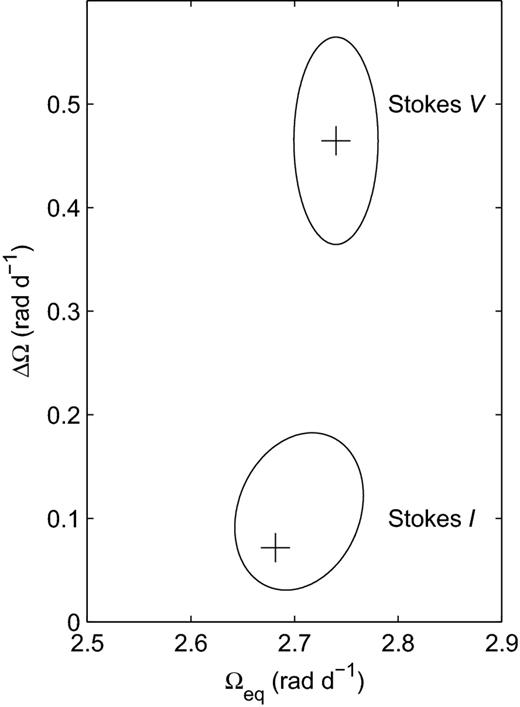
Differential rotation using Stokes I and V for HD 29615, including the associated variation ellipses (as explained in Section 5.3). The brightness (spot) features produce an equatorial rotational velocity, Ωeq, of 2.68|$_{-0.02}^{+0.06}$| rad d− 1 with rotational shear, ΔΩ, of 0.07|$_{-0.03}^{+0.10}$| rad d− 1. Using the magnetic features observed, HD 29615 has an equatorial rotational velocity, Ωeq, of 2.74 |$_{-0.04}^{+0.02}$| rad d− 1 with rotational shear, ΔΩ, of 0.48|$_{-0.12}^{+0.11}$| rad d− 1.
6.6 Surface differential rotation, rotation rate and convection zone depth
Barnes et al. (2005) showed a relationship between differential rotation (ΔΩ) and temperature, with increasing shear as a result of increasing temperature. Recent studies of G-dwarf stars such as HD 171488 (Marsden et al. 2006; Jeffers & Donati 2008; Jeffers et al. 2011) and HD 141943 (Marsden et al. 2011b) show significant levels of differential rotation beyond those observed by Barnes et al. (2005). HD 29615, like HD 171488, has extreme levels of rotational shear with a ΔΩ = 0.48|$_{-0.12}^{+0.11}$| rad d− 1. HD 171488 has a 1.33 d rotation period with a vsin i = 38 km s−1 whereas HD 29615 has a rotational period of 2.34 d with a vsin i = 19.6 km s−1. Given that both HD 171488 and HD 29615 have similar photospheric temperatures and age, it appears that rotation rate has limited effect on rotational shear, thereby supporting the observations by Barnes et al. (2005).
Küker et al. (2011), using theoretical models, demonstrated that the extreme surface shear of stars such as HD 171488 (and by implications HD 29615) can only be explained with a shallow convection zone. HD 171488 has a convection zone depth (CZD) of 0.206 R⋆ (0.233 R⊙; Jeffers et al. 2011) yet the CZD for HD 29615 was estimated to be 0.252 ± 0.011 R⋆, as determined from the stellar evolution models of Siess et al. (2000). The estimate for HD 29615 was based on the V − I colour index (van Leeuwen 2007) and the absolute magnitude, as determined from the maximum visual magnitude measured by the Hipparcos space mission. O'Neal, Saar & Neff (1996) concluded that on some heavily spotted stars, the observed maximum V magnitude underestimates the brightness of the unspotted star by ∼0.3–0.4 mag. For example, HD 106506 (Waite et al. 2011b) had a visual magnitude of ∼8.54 but the unspotted magnitude was determined to be 8.38 (using the imaging code). As there was limited knowledge of the fractional spottedness of many of the stars that had their differential rotation already determined by other authors, it was decided to use the maximum visual magnitude listed in the Hipparcos data base with the caveat that this possibly leads to an overestimate of the true CZD. This measurement for HD 29615 places additional constraints on the conclusion of the theoretical work of Küker et al. (2011) that extreme levels of differential rotation require a shallow convection zone.
7 CONCLUSIONS
From the results presented in this paper, HD 35296 and HD 29615 are both Sun-like stars whose moderately rapid rotation has led to very complex surface magnetic fields that exhibit high levels of chromospheric activity and surface differential rotation. This variation in the chromospheric activity, with rotational phase, was evidenced by modulation of the Ca ii H&K, Ca ii IRT and Hα spectral lines (HD 35296) and Hα emission (HD 29615). High levels of differential rotation were measured. The differential rotation on HD 29615 showed a significant discrepancy in shear values between spot and magnetic features. This is an extreme example of a variation also observed for other lower mass stars. There are indications that the magnetic field of HD 35296 appears to have undergone a minor reorganization of its field from 2007 to 2008 thereby demonstrating the evolving nature of the magnetic topology on this star. We conclude that the dynamo operating on both of these stars is similar to that of other more active, rapidly rotating stars and is most likely a distributed dynamo operating throughout the convection zone.
Thanks must go to the staff of the TBL and the AAT in their assistance in taking these data. This work has only been possible due to the brilliance of the late Meir Semel, from LESIA at Observatoire de Paris-Meudon. Sadly Meir passed away during 2012 but his memory and influence on spectropolarimetry will live on. The authors appreciate the time and dedication of the anonymous referee in producing constructive comments that has significantly improved this paper. This project has, in part, been supported by the Commonwealth of Australia under the International Science Linkages programme. SVJ and SBS acknowledge research funding by the Deutsche Forschungsgemeinschaft (DFG) under grant SFB 963/1 project A16. This project used the facilities of SIMBAD and Hipparcos. This research has made use of NASA's Astrophysics Data System.
