


Abstract
We present the results of an ensemble of SPH simulations that follow the evolution of pre-stellar cores for 0.2 Myr. All the cores have the same mass, and start with the same radius, density profile, thermal and turbulent energy. Our purpose is to explore the consequences of varying the fraction of turbulent energy, δsol, that is solenoidal, as opposed to compressive; specifically, we consider δsol = 1, 2/3, 1/3, 1/9 and 0. For each value of δsol, we follow 10 different realizations of the turbulent velocity field, in order also to have a measure of the stochastic variance blurring any systematic trends. With low δsol(<1/3), filament fragmentation dominates and delivers relatively high-mass stars. Conversely, with high values of δsol(>1/3) disc fragmentation dominates and delivers relatively low-mass stars. There are no discernible systematic trends in the multiplicity statistics obtained with different δsol.
1 INTRODUCTION
Understanding the origin of the stellar initial mass function (IMF; e.g. Kroupa 2001; Chabrier 2003, 2005) is one of the main unresolved problems in star formation. Because the physics regulating star formation (i.e. self-gravity, hydrodynamics, radiative transfer, magnetism, etc.) is highly non-linear, general cases can only be studied with numerical simulations. An intrinsic feature of the initial conditions for such simulations is the imposed turbulent velocity field, and since this velocity field is the source of the density fluctuations that spawn protostars, it is important to be clear about how it is defined.
Simulations of star formation usually follow one of two approaches. The first approach involves the simulation of isolated pre-stellar cores, i.e. the small (R ∼ 0.1 pc), dense (ρ ≳ 3 × 10− 20 g cm− 3) clumps of gas with sub-sonic or mildly trans-sonic internal turbulence, in which individual stars or small sub-clusters form (e.g. Bate 1998, 2000; Horton, Bate & Bonnell 2001; Matsumoto & Hanawa 2003; Goodwin & Whitworth 2004; Delgado-Donate, Clarke & Bate 2004a; Delgado-Donate et al. 2004b; Goodwin, Whitworth & Ward-Thompson 2004, 2006; Walch et al. 2009, 2010; Federrath et al. 2010b; Girichidis et al. 2011; Walch, Whitworth & Girichidis 2012). This approach has the advantage that individual simulations can be performed at high resolution with modest computational resource. Consequently, good statistics can be obtained by performing multiple realizations. However, it is still important to ensure that the initial conditions mimic reality as closely as is possible (e.g. Lomax et al. 2014).
The second approach involves the simulation of the much larger, less dense and more massive molecular clouds with highly supersonic internal turbulence, in which pre-stellar cores form (e.g. Klessen, Heitsch & Mac Low 2000; Bate 2009, 2012, 2014; Federrath & Klessen 2012). This approach has the advantage that the evolution includes both the formation of cores, and interactions between them, but it is not always feasible to perform more than one realization, and it remains to be seen if the initial conditions on this scale are critical.
In this paper, we consider the mildly trans-sonic turbulent velocity fields used to initiate simulations of individual pre-stellar cores. Specifically, we explore the effect of changing the fraction of turbulent energy, δsol, that is solenoidal as opposed to being compressive. Techniques for measuring the ratio of solenoidal to total turbulent energy have recently been developed (Brunt & Federrath 2014), but have not yet been widely applied. The values of δsol invoked in numerical simulations are seldom explicitly justified. The most common choices are δsol = 2/3 (thermal mixture, e.g. Walch et al. 2012; Lomax et al. 2014) and δsol = 1 (purely solenoidal, e.g. Bate 2009, 2012, 2014).
Previous numerical work on highly supersonic turbulence on molecular cloud scales (e.g. Federrath & Klessen 2012) indicates that compressive turbulence can deliver star formation rates up to 10 times higher than solenoidal turbulence. Numerical simulations of very massive cores with M = 100 M⊙ and R = 0.1 pc (Girichidis et al. 2011) also show that compressive turbulence accelerates the onset of star formation relative to solenoidal turbulence. Here, we study this issue on the much smaller scale of the pre-stellar cores typically seen in nearby star-forming regions (e.g. Ophiuchus), where the turbulence is a lot less vigorous.
In Section 2, we detail the initial conditions used for the simulations. In Section 3, we describe the numerical method and the constitutive physics. In Section 4, we present the results, and in Section 5 we summarize our conclusions.
2 INITIAL CONDITIONS
All the simulations presented here start with a spherical core having total mass M = 3 M⊙, radius R = 3000 au and non-thermal velocity dispersion σnt = 0.44 km s−1. These values are similar to those of the SM1 core in the Oph-A clump within the L1688 (Ophiuchus) cloud.1 The initial background temperature is set to 10 K.
2.1 Modified random turbulent velocity field
2.1.1 Standard random turbulent velocity field
2.1.2 Modifications to the longest wavelength modes
2.1.3 Helmholtz decomposition
2.1.4 Particle velocities
Having defined all the velocity modes, we use the fast Fourier transform library FFTW (Frigo & Johnson 2005) with kmax = 64 to compute a gridded velocity field |$\boldsymbol {v}(\boldsymbol {x})$| on −2R ≤ x1, x2, x3 ≤ +2R, and the velocities from the central eighth of the volume are then mapped on to the SPH particles.
2.2 Density profile
Many observations (e.g. Alves, Lada & Lada 2001; Harvey et al. 2001; Kirk, Ward-Thompson & André 2005; Lada et al. 2008; Roy et al. 2014) suggest that the critical Bonnor–Ebert sphere provides a good fit to the column-density profile of a pre-stellar core, even if the core is not in hydrostatic equilibrium. We therefore set the core density profile to |$\rho (\xi )=\rho _{c}\,{e}^{-\psi (\xi )}$|, where |$\rho _{c}$| is the central density, ψ(ξ) is the isothermal function and ξ is the dimensionless radius, i.e. ξ = 6.451(r/3000 au).
2.3 Parameter space
3 NUMERICAL METHOD
Core evolution is simulated using the seren ∇h-SPH code (Hubber et al. 2011), with η = 1.2 (so a particle typically has 57 neighbours). Gravitational forces are computed using a tree, and the Morris & Monaghan (1997) formulation of time-dependent artificial viscosity is invoked. In all simulations, the SPH particles have mass msph = 10−5 M⊙, so the opacity limit (∼3 × 10⁻³ M⊙) is resolved with ∼300 particles. Gravitationally bound regions with density higher than ρsink = 10−9 g cm−3 are replaced with sink particles (Hubber, Walch & Whitworth 2013). Sink particles have radius rsink ≃ 0.2 au, corresponding to the smoothing length of an SPH particle with density equal to ρsink. The equation of state and the energy equation are treated with the algorithm described in Stamatellos et al. (2007).
Radiative feedback from sinks is also included. Each sink has a variable luminosity which follows the episodic accretion model described in Stamatellos, Whitworth & Hubber (2011b, also used in Stamatellos, Whitworth & Hubber 2012; Lomax et al. 2014). In this model, highly luminous, short-lived accretion episodes are separated by ∼104 yr of low-luminosity quiescent accretion (during which matter collects in the inner accretion disc until it is hot enough to become thermally ionized and couple to the magnetic field; then the magnetorotational instability delivers efficient outward angular momentum transport and the matter is dumped on to the star).
4 RESULTS
Each core is evolved for 0.2 Myr. This is roughly the predicted time between core–core collisions in Ophiuchus (André et al. 2007). The simulations do not include any mechanical feedback from sinks (e.g. outflows), so the star formation efficiency is high, roughly 0.8 < η < 1.0. Previous work (e.g. Matzner & McKee 2000; Federrath et al. 2014) demonstrates that outflows and jets can reduce star formation efficiency significantly.
4.1 Modes of fragmentation
As a core collapses, turbulence and self-gravity organize the matter into filaments. These filaments usually behave in one of two ways: (i) they feed material from the periphery of the core into its centre, forming a central star, or (ii) they fragment independently to form multiple stars, which then congregate in a small cluster near the centre of the core. An example of case (i) is shown in Fig. 1 and an example of case (ii) is shown in Fig. 2. In the sequel, we refer to this initial mode of star formation as filament fragmentation.
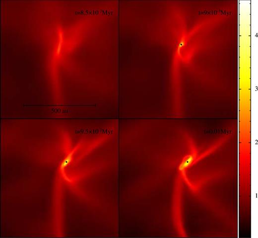
False-colour column-density images on the central 820 au × 820 au of the (x, y)-plane, from the simulation with |${\cal I}_{\rm seed}=3$| and δsol = 2/3, at times |$t=0.85,0.90,0.95\,{\rm and }\,1.00\times 10^4\,\mathrm{{\rm yr}}$|. The colour scale gives the logarithmic column density in units of g cm−2. Sink particles are represented by black dots. This is an example of filament fragmentation, where the filaments serve to deliver matter from the periphery of the core into the centre. Further evolution of this case is shown in Fig. 3.
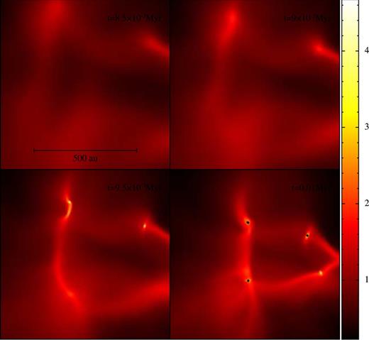
False-colour column-density images on the central 820 au × 820 au of the (x, y)-plane, from the simulation with |$\mathcal {I}_{\rm seed}=3$| and δsol = 0, at times t = 0.85, 0.90, 0.95 and 1.00 × 10⁴ yr. The colour scale gives the logarithmic column density in units of g cm−2. Sink particles are represented by black dots. This is an example of filament fragmentation, where the individual filaments fragment independently to produce an ensemble of stars. Further evolution of this case is shown in Fig. 4(a).
Once filament fragmentation has occurred, the remaining matter in the core envelope tries to accrete on to the star or cluster near the centre. If this matter has sufficient angular momentum, it forms circumstellar or circumsystem discs. Discs which are sufficiently massive (Toomre 1964) and are able to cool sufficiently fast (Gammie 2001) fragment to produce additional stars (e.g. Stamatellos & Whitworth 2008, 2009a,b; Stamatellos et al. 2011a). An example of this process is shown in Fig. 3. In the sequel, we refer to this second mode of star formation as disc fragmentation.
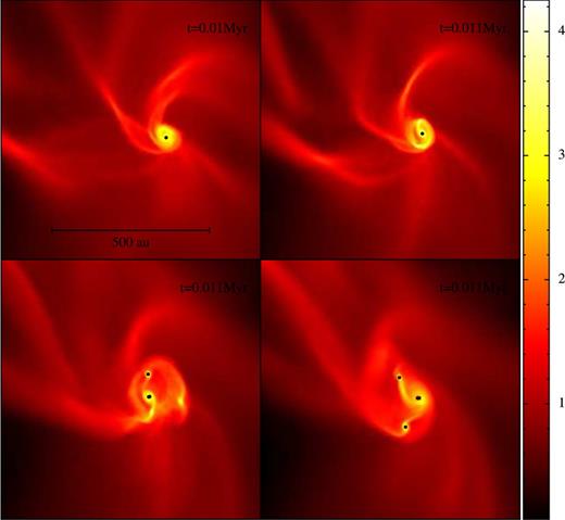
False-colour column-density images on the central 820 au × 820 au of the (x, z)-plane, from the simulation with |$\mathcal {I}_{{\rm seed}}=3$| and δsol = 2/3, at times t = 1.00, 1.05, 1.10 and 1.15 × 10⁴ yr. The colour scale gives the logarithmic column density in units of g cm−2. Sink particles are represented by black dots. This is an example of disc fragmentation. Further evolution of this case is shown in Fig. 4(d).
4.2 Influence of δsol on the dominant mode of fragmentation
Table 1 lists the number of stars that form by filament fragmentation, Nff, and the number that form by disc fragmentation, Ndf The distinction between the two modes is made by inspecting the simulation frames by eye. This table highlights the need to invoke multiple realizations with different random seeds, since, with a given δsol, the results can vary dramatically with |$\mathcal {I}_{\rm seed}$|. For example, with δsol = 1/9, only one star forms when |$\mathcal {I}_{\rm seed}=5$|, whereas 12 stars form when |$\mathcal {I}_{\rm seed}=10$|. This is because most of the turbulent energy is in large-scale modes which are defined by only a few wavevectors, and so the outcome is very sensitive to the random amplitudes of these modes.
The number of sinks formed by filament fragmentation, Nff, and by disc fragmentation, Ndf, in each simulation. Column 1 gives the random seed. Columns 2 and 3 give the number of sinks formed by filament fragmentation and by disc fragmentation when δsol = 0. Similarly, columns 4 and 5, 6 and 7, 8 and 9 and 10 and 11 give the same quantities when, respectively, δsol = 1/9, 1/3, 2/3 and 1. The second from last row gives total number of stars over all random seeds. The last row gives the relative fraction of stars formed via filament and disc fragmentation.
| δsol = 0 | δsol = 1/9 | δsol = 1/3 | δsol = 2/3 | δsol = 1 | ||||||
|---|---|---|---|---|---|---|---|---|---|---|
| |$\mathcal {I}_{\rm seed}$| | Nff | Ndf | Nff | Ndf | Nff | Ndf | Nff | Ndf | Nff | Ndf |
| 1 | 6 | 1 | 5 | 1 | 2 | 8 | 3 | 6 | 2 | 6 |
| 2 | 4 | 0 | 2 | 4 | 4 | 0 | 4 | 0 | 1 | 12 |
| 3 | 7 | 1 | 6 | 0 | 3 | 1 | 4 | 10 | 1 | 13 |
| 4 | 5 | 0 | 6 | 1 | 3 | 1 | 2 | 6 | 1 | 3 |
| 5 | 5 | 0 | 1 | 0 | 1 | 7 | 3 | 11 | 2 | 6 |
| 6 | 5 | 0 | 4 | 1 | 5 | 1 | 2 | 3 | 2 | 1 |
| 7 | 6 | 1 | 6 | 1 | 4 | 6 | 4 | 4 | 1 | 9 |
| 8 | 3 | 0 | 2 | 2 | 2 | 2 | 2 | 2 | 2 | 4 |
| 9 | 4 | 2 | 4 | 4 | 1 | 8 | 2 | 9 | 1 | 8 |
| 10 | 4 | 0 | 4 | 8 | 2 | 5 | 2 | 9 | 1 | 5 |
| Total | 49 ± 7 | 5 ± 2 | 40 ± 6 | 22 ± 5 | 27 ± 5 | 39 ± 6 | 28 ± 5 | 60 ± 8 | 14 ± 4 | 67 ± 8 |
| Fraction | 0.91 ± 0.04 | 0.09 ± 0.04 | 0.65 ± 0.06 | 0.35 ± 0.06 | 0.41 ± 0.06 | 0.59 ± 0.06 | 0.32 ± 0.05 | 0.68 ± 0.05 | 0.17 ± 0.04 | 0.83 ± 0.04 |
Fig. 4 shows the early stages of star formation with |$\mathcal {I}_{\rm seed}=3$| and different values of δsol. In Fig. 4(a), where δsol = 0, seven stars form by filament fragmentation, and then a single star by disc fragmentation. In Fig. 4(e), where δsol = 1, a single star forms by filament fragmentation, then 13 by disc fragmentation. Figs 4(b), (c) and (d) show how the number of stars formed by filament fragmentation tends to decrease, and the number of stars formed by disc fragmentation to increase, with increasing δsol. This trend is seen more clearly in Fig. 5 where the results are averaged over all values of |$\mathcal {I}_{\rm seed}$|. The average fraction of stars formed from a core by filament fragmentation decreases monotonically from ∼0.9 when δsol = 0 to ∼0.2 when δsol = 1. Conversely, the average fraction of stars formed from a core by disc fragmentation increases monotonically from ∼0.1 when δsol = 0 to ∼0.8 when δsol = 1. This is because predominantly compressive fields (low δsol) are characterized by shocks, and these are conducive to filament formation. Conversely, predominantly solenoidal fields (high δsol) are characterized by shearing motions, and these generate the angular momentum required for the formation of discs.
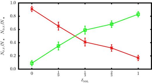
The fraction of stars formed by filament fragmentation (red ×s) and disc fragmentation (green |$\Box$|s) for different values of δsol, averaged over all values of |$\mathcal {I}_{\rm seed}$|. The error bars give the Poisson counting uncertainties.
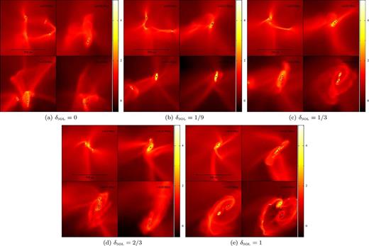
False-colour column-density images on the central 820 au × 820 au of the (x, y)-plane, from the simulations with |$\mathcal {I}_{\rm seed}=3$| and different values of δsol, at times t = 1.00, 1.25, 1.50 and 1.75 × 10⁴ yr. The colour scale gives the logarithmic column density in units of g cm−2. Sink particles are represented by black dots.
Table 1 also indicates that the total number of stars formed per core increases slightly with increasing δsol. When δsol = 0, a core spawns on average ∼5 stars; when δsol = 1, a core spawns on average ∼8 stars.
4.3 Influence of δsol on the stellar mass distribution
Fig. 6 shows the distribution of stellar masses formed with different values of δsol, integrated over all values of |$\mathcal {I}_{\rm seed}$|. Fig. 7 shows how the corresponding medians and interquartile ranges vary with δsol. We see that, as δsol is increased, the median decreases monotonically, from ∼0.6 M⊙ when δsol = 0, to ∼0.3 M⊙ when δsol = 1. For reference, Fig. 6 also shows the Chabrier (2005; hereafter C05) IMF (dashed red curve), and Fig. 7 shows the corresponding median and interquartile range (full and dashed horizontal red lines). However, we stress that we should not expect to reproduce the overall distribution of stellar masses observed in nature with simulated cores of a single mass, radius and non-thermal velocity dispersion, as treated here. We are simply seeking to establish what trends, if any, might derive from changing the mix of solenoidal and compressive modes in the imposed turbulent velocity field.
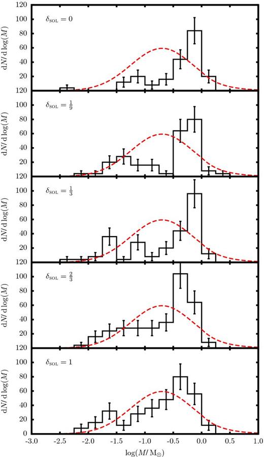
The black histograms show un-normalized stellar mass distributions, integrated over all values of |$\mathcal {I}_{\rm seed}$|, for different values of δsol. The error bars give the Poisson counting uncertainties. The red dashed lines show the Chabrier (2005) IMF, scaled to the area of the δsol = 1 histogram.
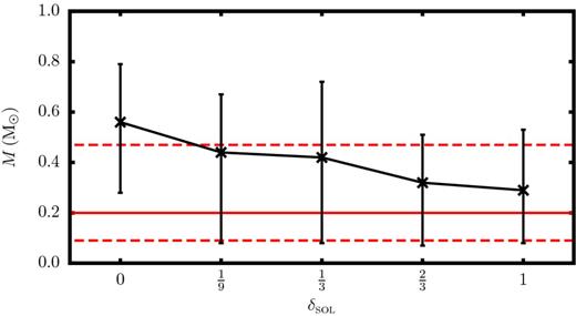
The black ×s give the median stellar mass, and the vertical black bars give the corresponding interquartile range, for different values of δsol, integrated over all values of |$\mathcal {I}_{\rm seed}$|. The solid and dashed horizontal red lines give the median and IQR for the Chabrier (2005) IMF.
The decrease in median mass that results from increasing δsol can be attributed directly to the shift from filament fragmentation when δsol is low to disc fragmentation when δsol is high. When δsol is low, compressive turbulent modes create filaments, and these can be very effective at feeding matter from the periphery of the core, into the centre, where it forms a relatively massive star. Conversely, when δsol is high, solenoidal turbulent modes create discs around existing stars, and these discs tend to fragment to produce large numbers of low-mass companion stars.
4.4 Multiplicity statistics
4.4.1 Multiplicity frequency
Multiplicity frequencies and pairing factors, for different values of δsol, integrated over all values of |$\mathcal {I}_{\rm seed}$|. Uncertainties on mf are given by |$\Delta {\rm mf}=\sqrt{{\rm mf}\,(1-{\rm mf})/(N_{{\rm sys}})}$| where Nsys is the total number of systems. Uncertainties on pf are assumed to satisfy Δpf > pf Δmf/mf (see footnote 3 for discussion).
| δsol = 0 | |$\delta _{\rm sol} = \frac{1}{9}$| | |$\delta _{\rm sol} = \frac{1}{3}$| | |$\delta _{\rm sol} = \frac{2}{3}$| | δsol = 1 | |
|---|---|---|---|---|---|
| |$N_ {sys}$| | 32 | 34 | 51 | 61 | 55 |
| mf | 0.28 | 0.32 | 0.20 | 0.23 | 0.29 |
| Δmf | 0.08 | 0.08 | 0.06 | 0.05 | 0.06 |
| pf | 0.63 | 0.82 | 0.29 | 0.42 | 0.49 |
| Δpf | >0.18 | >0.20 | >0.08 | >0.10 | >0.10 |
4.4.2 Orbital properties
The number of multiple systems formed in the simulations is too small to allow us to consider in detail how the distributions of orbital properties vary with δsol. There is some tenuous evidence that, as δsol increases, the orbital eccentricities increase and the mass ratios decrease – in other words, more compressive turbulence promotes more circular orbits and more closely matched companion masses – but this is a very weak result. However, we can examine the combined distributions of semimajor axis a, mass ratio q and eccentricity e. Fig. 8 shows the distribution of a, q and e alongside analytic fits. The parameters of these fits are given in Table 3. These distributions include all the orbits of hierarchical systems.

Histograms showing the distribution of orbital properties integrated over all simulations (i.e. all δsol and |$\mathcal {I}_{\rm seed}$|). The top panel shows the distribution of |$\log _{_{10}}(a/{\rm au})$|, where a is the semimajor axis. The middle panel shows the distribution of mass ratios, q. The bottom panel shows the distribution of eccentricities, e. The red dashed lines are analytical fits to the data; fitting parameters are given in Table 3.
Fitted multiplicity parameters integrated over all simulations (i.e. all δsol and |$\mathcal {I}_{\rm seed}$|). μa and σa are the mean and standard deviation of |$\log _{_{10}}(a/{\rm au})$|, where a is the semimajor axis. γ is the mass ratio distribution parameter dN/dq ∝ qγ. ϵ is the eccentricity distribution parameter dN/de ∝ (1 − e)ϵ. γ and ϵ are calculated using maximum likelihood estimation.
| μa | σa | γ | ϵ |
|---|---|---|---|
| 0.7 ± 0.1 | 1.0 ± 0.1 | 1.6 ± 0.2 | 1.6 ± 0.2 |
| μa | σa | γ | ϵ |
|---|---|---|---|
| 0.7 ± 0.1 | 1.0 ± 0.1 | 1.6 ± 0.2 | 1.6 ± 0.2 |
The semimajor axes range from 0.2 to 2000 au. The lower limit is set by the resolution of the simulations (i.e. the radius of a sink particle). The upper limit is compatible with observations of young embedded populations (e.g. Taurus, Ophiuchus, etc.; King et al. 2012a,b).
If we fit the distribution of mass ratios with a power law of the form dN/dq ∝ qγ, we obtain γ = 1.6 ± 0.2, implying a strong preference for companions of comparable mass. Young embedded populations also show a preference for companions of comparable mass, but it is somewhat weaker, viz. 0.2 ≲ γ ≲ 1 (Duchêne & Kraus 2013). To establish whether the observations could be fit more closely with a specific value of δsol would require a much larger ensemble of simulations.
If we fit the distribution of eccentricities with a reverse power law of the form dN/de ∝ (1 − e)ϵ, we obtain ϵ = 1.6 ± 0.2, implying a preference for low eccentricity, similar to the preferentially circular orbits of field M-dwarfs (see Duchêne & Kraus 2013, fig. 4).
5 DISCUSSION AND CONCLUSIONS
5.1 Limitations
First, we stress that the work reported here is a numerical experiment, not an attempt to capture all the processes that occur in real pre-stellar cores. In particular, we have simulated cores with a single mass, single radius, single non-thermal velocity dispersion and single density profile. The only parameters varied are the fraction of turbulent energy that is solenoidal, δsol, and the random seed that delivers different realizations, |${\cal I}_{\rm seed}$|. Therefore, the results cannot be applied to all pre-stellar cores. Indeed, the results reported by Lomax et al. (2014) suggest that cores with masses ≪1 M⊙ tend to form single stars, whilst cores with ≳1 M⊙ tend to form discs and filaments which fragment into multiple stars. The results presented here relate to the latter case.
Secondly, we have not included magnetic fields in the simulations. The three-dimensional structure of a core's magnetic field is extremely difficult to extract from observations, and the evolution of the magnetic field requires the treatment of non-ideal MHD effects, along with the detailed ionization chemistry of the matter. It is therefore beyond the scope of this investigation.
5.2 Implications for star formation
δsol can only be determined observationally if one has the detailed three-dimensional velocity field, or if one has the detailed one-dimensional velocity field and a model, for example, assumed statistical isotropy of the velocity field (see Brunt & Federrath 2014). On the scale of cores, one does not have this information (because of instrumental limitations, selection effects and confusion), and one cannot make these assumptions.
The turbulent velocity field in a core is largely determined by the flows that create it. If a core is created by turbulent fragmentation (e.g. Padoan & Nordlund 2002; Hennebelle & Chabrier 2008, 2009) and there is a large inertial range between the scale at which the turbulent energy is injected (say by galactic shear) and the scale of the core, δsol is likely to approach its thermal value, i.e. 2/3, and in this case disc fragmentation should be important. However, in reality there is probably not a clear division between the scale of energy injection and the inertial range leading to core formation; rather, turbulent energy is injected on many scales, including some that are smaller than, or comparable with, the core scale. In particular, when (if) a core condenses directly out of a shell swept up by an expanding nebula (H ii region, stellar-wind bubble or supernova remnant), there may be a predominance of compressive turbulent energy, a very small inertial range and hence a low value of δsol, not so much disc fragmentation, and not so many low-mass stars.
5.3 Comparison with similar work
Girichidis et al. (2011) present adaptive mesh refinement simulations on scales intermediate between the molecular clouds simulated by, for example, Bonnell, Clark & Bate (2008), and the cores treated in this work. They find that star formation occurs 25 per cent earlier (with respect to the start time of the simulation) when the velocity field is purely compressive, as opposed to solenoidal. They do not report an increase in the number of low-mass stars or brown dwarfs formed when the turbulence is purely solenoidal. This may be because their minimum resolvable length scale is tens of au, which is insufficient to capture the dynamics of disc fragmentation.
5.4 Summary
We have shown that the collapse and fragmentation of a core is influenced by the fraction of turbulent energy that is solenoidal, δsol, and hence – by default – by the fraction that is compressive. Specifically, as δsol is increased from 0 (purely compressive) to 1 (purely solenoidal), the proportion of stars that form by filament fragmentation decreases and the proportion that form by disc fragmentation increases; at the same time the number of stars formed increases, and their mean mass decreases. The formation of massive circumstellar discs requires δsol > 1/3. With the limited number of simulations that we have performed, we have been unable to establish any robust systematic trends in the multiplicity statistics that derive from varying δsol.
OL and APW gratefully acknowledge the support of a consolidated grant (ST/K00926/1) from the UK STFC. We also thank the considerate and constructive comments from the referee. This work was performed using the computational facilities of the Advanced Research Computing @ Cardiff (ARCCA) Division, Cardiff University. All false-colour images have been rendered with splash (Price 2007).
Using 1.3-mm dust continuum observations, Motte, Andre & Neri (1998) estimate that SM1 has a mass of 3.2 M⊙ and an azimuthally averaged full width at half-maximum of 3600 au. André et al. (2007) measure the velocity width of the N2H+ (1−0) line and estimate that the three-dimensional non-thermal velocity dispersion is 0.45 km s−1.
Strictly speaking, a power law exponent of −4 (Burgers turbulence) is only appropriate for highly supersonic turbulence (see Federrath 2013). At sonic and trans-sonic speeds, the exponent is likely to be between −4 and −11/3 (Kolmogorov turbulence). However, with both exponents, the turbulent energy is strongly concentrated at the longest wavelengths, and so the precise choice of exponent is not critical.
mf depends only on two numbers, S and |$B+T+Q+\cdots =(N_ {sys}-S)$|. In contrast, pf depends on S, B, T, Q, etc.; if we count up to sextuples, then six numbers. The higher the order of the system being counted, |${\cal O}$|, the smaller the number of systems and hence the higher the fractional Poisson uncertainty. However, these systems are given higher weight in the numerator of pf, i.e. |$w_{_{\cal O}}=({\cal O}-1)$|, so their individual uncertainties are compounded in a way that they are not in mf.
