


Abstract
We report the discovery of an ∼1.5 × 10⁻⁴ Hz (∼2 h) X-ray quasi-periodic oscillation (QPO) in the active galaxy MS 2254.9−3712, using an ∼70 ks XMM–Newton observation. The QPO is significantly detected (∼3.3σ) in the 1.2–5.0 keV band only, connecting its origin with the primary X-ray power-law continuum. We detect a highly coherent soft lag between the 0.3–0.7 keV and 1.2–5.0 keV energy bands at the QPO frequency and at a frequency band in a 3:2 ratio, strongly suggesting the presence of a QPO harmonic. An iron Kα reverberation lag is found at the harmonic frequency, indicating the reflecting material subtends some angle to the primary continuum, which is modulated by the QPO mechanism. Frequency-resolved spectroscopy reveals the QPO and harmonic to have a hard energy dependence. These properties of the QPO variability, together with the current black hole mass estimate, MBH ∼ 4 × 10⁶ M⊙, are consistent with the QPO originating from the same process as the high-frequency QPO phenomenon observed in black hole X-ray binaries. Principle component analysis reveals the spectral variability in MS 2254.9−3712 is similar to that of the active galaxy RE J1034+396, a source which also displays an X-ray QPO. This suggests a distinct spectral-variability pattern for accreting black holes when in a state where QPOs are present.
1 INTRODUCTION
Black hole X-ray binaries (BHBs; |${M_{{\rm BH}}}\sim 10 {\,\mathrm{M}_{{\odot}}}$|) display both low-frequency (∼0.1–30 Hz) and high-frequency (∼40–450 Hz) quasi-periodic oscillations (LFQPOs; HFQPOs) in their X-ray power spectra (PSD; see e.g. Remillard & McClintock 2006 for a review). HFQPOs are the fastest coherent features observed in accreting BHs and their high frequencies suggest an origin in the innermost regions of the accretion flow. Understanding this phenomenon will then provide important information on the BH mass and spin as well as the structure of the strongly-curved space–time close to the event horizon (e.g. Milsom & Taam 1997; Nowak et al. 1997; Stella, Vietri & Morsink 1999; Wagoner 1999; Abramowicz & Kluźniak 2001; Rezzolla et al. 2003; Das & Czerny 2011).
A scale invariance of the accretion process (e.g. Shakura & Sunyaev 1973; Mushotzky, Done & Pounds 1993) implies that QPOs should also be present in active galactic nuclei (AGN; |${M_{{\rm BH}}}\gtrsim 10^{6} {\,\mathrm{M}_{{\odot}}}$|). For a BH mass ratio MBHB/MAGN = 10−5, the expected frequency of LFQPOs in AGN is fLFQPO ≳ 10−5 (i.e. time-scales of ≳100 ks). LFQPOs are therefore not expected to be easily detected in AGN with existing data (see Vaughan & Uttley 2005). The analogous HFQPOs in AGN are expected to occur at fHFQPO ≳ 5 × 10⁻³ Hz (i.e. time-scales of ≳200 s), well within the temporal passband of e.g. XMM–Newton. If detected in AGN, the longer periodicity means, we can study the QPO on the level of individual periods, given sufficient data quality, providing a better window into the HFQPO phenomenon across the BH mass scale.
QPOs have been notoriously difficult to detect in AGN, with many early ‘detections’ disfavoured due to an inadequacy in modelling the underlying broad-band noise (Vaughan 2005; Vaughan & Uttley 2006; González-Martín & Vaughan 2012 and references therein). An ∼200 s QPO (most likely an HFQPO) was detected in the tidal disruption event Swift J164449.3+573451 (Reis et al. 2012). Recently, an ∼3.8 h QPO was reported in 2XMM J123103.2+110648 (Lin et al. 2013). The low BH mass (|${M_{{\rm BH}}}\sim 10^{5} {\,\mathrm{M}_{{\odot}}}$|) and 50 per cent rms variability (typically ≳15 per cent for LFQPOs in BHBs; e.g. Remillard & McClintock 2006) led the authors to associate this with the LFQPO phenomenon. The first robust AGN HFQPO detection came from the Seyfert galaxy RE J1034+396, with an ∼1 h periodicity (Gierliński et al. 2008). Recently, we showed that the QPO is present in five years of XMM–Newton observations of RE J1034+396 (Alston et al. 2014b, hereafter A14). The frequency of the QPO has remained constant in this time, although it is now only detected in the 1.0–4.0 keV band. This strengthens the association of the QPO with the primary (hot, optically thin) Comptonizing corona, as observed in BHBs (e.g. Remillard & McClintock 2006).
Accreting BHs display hard lags at low frequencies – where variations in harder energy bands are delayed with respect to softer energy bands (Miyamoto & Kitamoto 1989; Nowak et al. 1999a,b; Vaughan et al. 2003b; McHardy et al. 2004; Arévalo, McHardy & Summons 2008; Kara et al. 2013a; Alston, Done & Vaughan 2014a; Lobban, Alston & Vaughan 2014). The leading model for the origin of the hard lags is the radial propagation of random accretion rate fluctuations through a stratified corona (e.g. Lyubarskii 1997; Churazov, Gilfanov & Revnivtsev 2001; Kotov, Churazov & Gilfanov 2001, Arévalo & Uttley 2006).
A switch from hard (propagation) lags at lower frequencies to soft (reverberation) lags at higher frequencies has now been observed in ≳20 AGN (e.g. Fabian et al. 2009; Emmanoulopoulos, McHardy & Papadakis 2011; Zoghbi, Uttley & Fabian 2011; Alston, Vaughan & Uttley 2013; Cackett et al. 2013; De Marco et al. 2013a; Kara et al. 2013b; Alston et al. 2014a). A consistent picture is emerging where the soft lag represents the reverberation signal as the primary X-ray emission is reprocessed by the inner accretion disc itself (e.g. Fabian et al. 2009, see Uttley et al. 2014 for a review). Further evidence for this scenario comes from the corresponding detection of high-frequency iron Kα lags (e.g. Zoghbi et al. 2012, 2013; Kara et al. 2013c) and Compton hump reverberation lags above 10.0 keV observed with NuSTAR (Zoghbi et al. 2014; Kara et al. 2015). High-frequency soft lags have also been observed in an ultraluminous X-ray source (Heil & Vaughan 2010; De Marco et al. 2013b) and one hard state BHB (Uttley et al. 2011).
The time lags of HFQPOs in BHBs have also been studied, with Cui (1999) finding a hard lag in the 67 Hz QPO in GRS 1915+105. Recently, Méndez et al. (2013) performed a systematic study of HFQPO time lags in a sample of four BHBs. They found a hard lag in all QPOs with the exception of the 35 Hz QPO in GRS 1915+105 which displays a soft lag that increases with increasing energy separation. The physical meaning of these HFQPO time lags is still uncertain. However, they provide an extra diagnostic for identifying HFQPOs and for understanding their physical origin.
In this paper, we present the significant detection of a QPO in the AGN MS 2254.9−3712 and explore several aspects of the QPO spectral variability. MS 2254.9−3712 is a nearby (z = 0.039; Stocke et al. 1991), X-ray bright (log (LX) = 43.29 erg s−1; Grupe et al. 2004) and ‘unabsorbed’ (NH < 2 × 1022 cm−1; Grupe et al. 2004) radio quiet (Shields et al. 2003) narrow line Seyfert 1 (NLS1) galaxy [FWHM(Hβ) ∼ 1500 km s−1; Grupe et al. 2004].
The central BH mass in MS 2254.9−3712 derived from the empirical RBLR − λLλ(5100 Å) relation (e.g. Kaspi et al. 2000) is |${M_{{\rm BH}}}\sim 4 \times 10^{6}$| (Grupe et al. 2004, 2010). The BH mass derived from the |${M_{{\rm BH}}}{\rm -}\sigma$| relation (Tremaine et al. 2002) using σ(O iii) is estimated as |${M_{{\rm BH}}}\sim 10^{7}$| (Shields et al. 2003). The Eddington rate estimated from λLλ(5100 Å) is |$L_{\rm Bol}/ {L_{\rm Edd}}= 0.24$| (Grupe et al. 2004, 2010). However, Wang (2003) suggests MS 2254.9−3712 is accreting at super-Eddington rate (|${\dot {M}} / {\dot{m}_{\rm Edd}} > 1$|). They found that super-Eddington accretion can lead to a limit relation between the BH mass and the FWHM of the broad lines, indicating that super-Eddington accretors radiate close to their Eddington luminosity, but accrete above the Eddington limit (see also Collin & Kawaguchi 2004).
The structure of this paper is as follows: in Section 2, we describe the observations and data reduction; in Section 3, we present the power spectral analysis and QPO identification. We explore the time delays, frequency-dependent energy spectra and principle component analysis (PCA) in Section 4. In Section 5, we discuss these results and the QPO identification.
2 OBSERVATIONS AND DATA REDUCTION
We make use of the single ∼70 ks XMM–Newton observation of MS 2254.9−3712 from 2005 (oBS ID: 0205390101). For the timing analysis in this paper, we use both the EPIC-pn (European Photon Imaging Camera; Strüder et al. 2001) and EPIC-MOS data. These observations were taken in small window mode. The MOS data are split into three exposures, of which we make use of exposure 3 only with duration 62 ks. We processed the observation data files following standard procedures using the XMM–Newton Science Analysis System (sas v13.5.0), using the most recent calibration files as of 2014 October. We processed the data using the filtering conditions PATTERN = 0–4 (<=12 for MOS) and FLAG = 0 (#XMMEA_EM for MOS). We extract source light curves from a 20 arcsec circular region. The background was taken from a large rectangular region on the same chip, approximately 15 times larger than the source region and placed away from the chip edges. Various background regions were also used in the following analysis, and the choice of background region was found to have no significant effect on the results.
For the PSD analysis in Section 3, we filtered soft proton flares using a threshold of 0.5 count s−1 in the 10.0–12.0 keV background light curve. We linearly interpolate across any gaps less than 500 s and add Poisson noise. This background rate cut removes the period of high background flaring at the start of the observation giving 58 ks of high-quality data where the EPIC-pn and EPIC-MOS overlap. This ensures the highest signal-to-noise ratio (S/N) light curves in the PSD analysis, which is most sensitive to uncorrelated (Poisson) noise. After accounting for the flares at the beginning of the observation, the interpolation fraction is negligible in the remaining 58 ks.
For the remaining analysis in Section 4 onwards, we filter the data for soft proton flares using a threshold of 2 count s−1 in the 10.0–12.0 keV background light curve. Again, we linearly interpolate across any short gaps and add Poisson noise, although the interpolation fraction was negligible using this rate cut. This rate cut allows for the full 70 ks of EPIC-pn data to be used in the cross-spectral analysis in Section 4, enabling us to probe to lower frequencies and increasing the frequency resolution.
The resulting full background subtracted source light curves (with Δt = 200 s for plotting purposes) for several energy bands are shown in Fig. 1 (blue), as well as the background light curve (grey). We show only the 1.2–5.0 keV MOS band for illustrative purposes. With a mean count rate of 1.35 count s−1 in the 0.3–10.0 keV band, pile-up is negligible in this observation. A binsize Δt = 100 s is used in the timing analysis throughout.
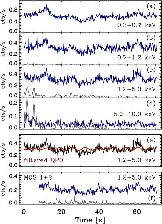
Background-subtracted source (blue) and background (grey) EPIC-pn light curves for the 0.3–0.7 keV (a), 0.7–1.2 keV (b), 1.2–5.0 keV (c) and 5.0–10.0 keV (d) bands. A binsize of Δt = 200 s is used for plotting purposes. The QPO filtered 1.2–5.0 keV band light curve (red) and original (black) are shown in panel (e). A bandpass filter with width ±20 per cent the QPO frequency was applied, see Section 3 for details. Panel (f) shows the combined EPIC-MOS 1+2 background-subtracted source (blue) and background (grey) 1.2–5.0 keV band light curves.
3 ENERGY-DEPENDENT POWER SPECTRUM
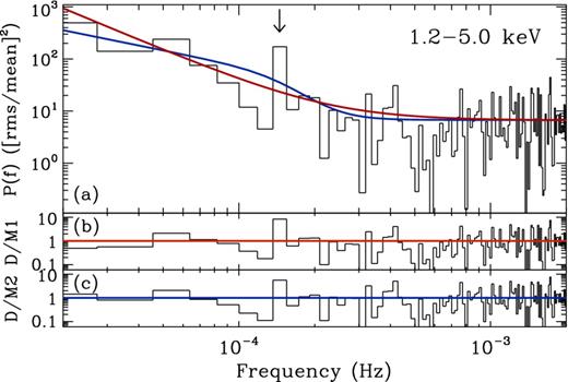
The PSD was estimated using the standard method of calculating the periodogram (e.g. Priestley 1981; Percival & Walden 1993), with an [rms/mean]2 normalization (e.g. Vaughan et al. 2003b). Motivated by the PSD analysis in A14, we estimated the periodogram in four energy bands; 0.3–0.7, 0.7–1.2, 1.2–5.0 and 5.0–10.0 keV. The PSD of the 1.2–5.0 keV band is shown in Fig. 2. The energy bands were chosen in order to investigate the association of a QPO feature with a particular spectral component, whilst maintaining a high S/N PSD.
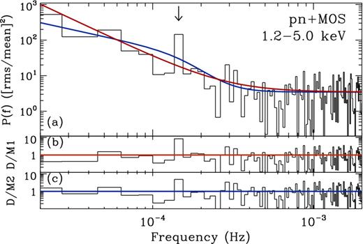
The 1.2–5.0 keV band PSD and model fits are shown in panel (a), for model 1 (red) and model 2 (blue). The data/model residuals for models 1 and 2 are shown in panels (b) and (c), respectively.
We fitted the PSDs with simple continuum models and searched for significant data/model outliers using the maximum likelihood method of Vaughan (2010, hereafter V10). The fitting procedure distinguishes between continuum models before testing the preferred continuum model for deficiencies that indicate the presence of a significant narrow coherent feature. In this way, we are sensitive to QPOs that are constrained to one frequency bin width. The details of the model fitting are given in A14 and we refer the reader to V10 (and references therein) for a full discussion.
A likelihood ratio test (LRT) statistic (equation 22 of V10) was used to select between the continuum models, H0 and H1 (e.g. Protassov et al. 2002; V10). Following V10, the null-hypothesis model H0 was rejected using the criterion pLRT < 0.01, which the simulation results of V10 suggest is a conservative estimate.
Once the preferred continuum model has been selected, the presence of narrow coherent features is investigated using two test statistics. Markov chain Monte Carlo simulations were used to find the test statistic distribution and the associated posterior predictive p-value (ppp). The overall model fit is assessed using the summed square error, TSSE (equation 21 of V10), which is analogous to the traditional chi-square statistic. A small pSSE indicates an inadequacy in the continuum modelling. Significant outliers are investigated using |$T_{\rm R} = {\rm max}_j \hat{R}_j$|, where |$\hat{R} = 2I_{j} / \hat{S}_j$| and Ij is the observed periodogram and Sj is the model power spectrum at frequency νj. A small pR indicates that the largest outlier is unusual under the best-fitting continuum model and the presence of a QPO is inferred.
In model 2, νbend was originally set to a value 1.5 × 10⁻⁴ Hz from the best-fitting value found in González-Martín & Vaughan (2012, hereafter GMV12). The prior distributions on all model parameters have a 3σ dispersion around the mean level (see V10, section 9.4). The results of the PSD fitting are shown in Table 1, along with the 68.3 per cent (1σ) confidence intervals on model parameters.
Results of model fits to the pn+MOS PSDs. Column (1) shows the energy range, column (2) shows the ppp for the LRT between the null hypothesis and alternative hypothesis. Columns (3) and (4) show the ppp for TSSE and TR, respectively. Column (5) shows the ratio Rj = 2Ij/Sj, where j is the QPO frequency, fQPO = 1.5 × 10⁻⁴ Hz and (6) is the absolute rms at fQPO. Columns (7)–(10) show the best-fitting model parameters with their 68.3 per cent confidence intervals. For Model 2, column (8) shows the αhigh parameter.
| En band | pLRT | pSSE | pR | Rj | rms(fQPO) | log(N) | α | log(νbend) | Pnoise |
|---|---|---|---|---|---|---|---|---|---|
| (keV) | (per cent) | (Hz) | |||||||
| (1) | (2) | (3) | (4) | (5) | (6) | (7) | (8) | (9) | (10) |
| Model 1 | |||||||||
| 0.3–0.7 | 0.1762 | 0.7750 | 0.2182 | 5 | 3 | |$-9.2^{+1.1}_{-1.2}$| | |$2.6^{+0.4}_{-0.3}$| | – | |$0.75^{+0.04}_{-0.04}$| |
| 0.7–1.2 | 0.1196 | 0.0435 | 0.0748 | 9 | 4 | |$-8.5^{+1.3}_{-1.5}$| | |$2.4^{+0.4}_{-0.3}$| | – | |$1.07^{+0.05}_{-0.05}$| |
| 1.2–5.0 | 0.0012 | 0.0010 | 0.0010 | 18 | 6 | |$-9.2^{+1.2}_{-1.3}$| | |$2.5^{+0.4}_{-0.3}$| | – | |$0.85^{+0.04}_{-0.04}$| |
| Model 2 | |||||||||
| 0.3–0.7 | 0.2270 | 0.7760 | 0.7828 | 5 | 3 | |$-2.2^{+0.3}_{-0.4}$| | |$4.6^{+0.4}_{-0.7}$| | |$-4.09^{+0.10}_{-0.15}$| | |$0.76^{+0.04}_{-0.03}$| |
| 0.7–1.2 | 0.6448 | 0.0452 | 0.0757 | 6 | 4 | |$-2.5^{+0.4}_{-0.4}$| | |$4.1^{+0.6}_{-0.7}$| | |$-3.92^{+0.11}_{-0.15}$| | |$1.06^{+0.04}_{-0.05}$| |
| 1.2–5.0 | 0.5230 | 0.0252 | 0.0384 | 10 | 6 | |$-2.7^{+0.4}_{-0.4}$| | |$4.9^{+0.7}_{-0.7}$| | |$-3.74^{+0.24}_{-0.25}$| | |$0.85^{+0.03}_{-0.04}$| |
The 1.2–5.0 keV band is the only energy band to display a significant outlier at ∼1.5 × 10⁻⁴ Hz (pSSE = 0.001; pR = 0.001), with Model 1 preferred (pLRT = 0.0012). Fig. 2 shows the best-fitting models to the 1.2–5.0 keV band. Despite Model 1 being preferred, the p-values of Model 2 are moderately low (pSSE = 0.03; pR = 0.03), indicating the outlier at ∼1.5 × 10⁻⁴ Hz is unusual under the best-fitting Model 2. In Appendix A, we show the individual pn and MOS 1.2–5.0 keV PSDs.
The best-fitting models to the 0.3–0.7, 0.7–1.2 keV bands are shown in Figs 3 and 4, respectively. Although no formally significant outlier was detected in these two bands, some structure in the PSD can be seen at ∼1.5 × 10⁻⁴ Hz. The 5.0–10.0 keV band PSD is dominated by Poisson noise and hence we do not show it here.
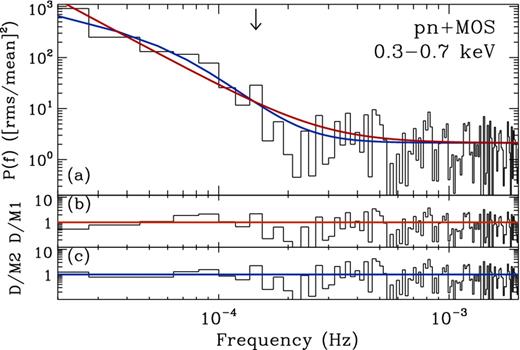
The 0.3–0.7 keV band PSD and model fits are shown in panel (a), for model 1 (red) and model 2 (blue). The data/model residuals for models 1 and 2 are shown in panels (b) and (c), respectively.
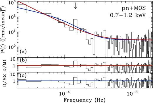
The 0.7–1.2 keV band PSD and model fits are shown in panel (a), for model 1 (red) and model 2 (blue). The data/model residuals for models 1 and 2 are shown in panels (b) and (c), respectively.
The QPO at ∼1.5 × 10⁻⁴ Hz is confined to one frequency bin, making the QPO highly coherent. The quality factor Q = ν/Δν is ∼8. The QPO rms fractional variability for each band is given in column 6 of Table 1. A value of 6 per cent is observed in the 1.2–5.0 keV band. If we assume the narrow outliers at ∼1.5 × 10⁻⁴ Hz in the two softer bands also indicate the presence of a QPO, then we observe an increase in the QPO rms with increasing energy band.
The QPO does not appear as apparent in the light curve compared to those observed in BHBs or the 1.0–4.0 keV band in RE J1034+396 (see A14 fig. 1). To illustrate the QPO, we apply a bandpass filter to the 1.2–5.0 keV light curve, with a frequency width ±30 per cent of the QPO frequency. This removes the variations outside of the filter window, allowing the variations on the time-scale of the filter bandpass to be seen. The filtered light curve is plotted in Fig. 1 panel (e), where the quasi-periodic nature of the light curve is now apparent. We note here, however, that a narrow filter applied to a pure noise signal will also produce a quasi-sinusoidal time series, except the amplitude of the oscillation will be greatly reduced. The deviation from a quasi-periodic signal in the 1.2–5.0 keV light curve is most likely due to the red noise nature of the broad-band noise which contributes a substantial amount of power at low frequencies (see Fig. 2). These long time-scale trends then wash out the quasi-periodic signal. The amplitude of the broad-band noise below the observed QPO in the 1.0–4.0 keV band in RE J1034+396 is much smaller than in MS 2254.9−3712, and hence why the QPO is apparent in the light curve of RE J1034+396 (see A14 fig. 1).
4 THE FREQUENCY-DEPENDENT VARIABILITY
4.1 The cross-spectrum
In this section, we explore the cross-spectral products (PSDs, coherence and time delays) between the 1.2–5.0 keV band and the two softer bands. In this way, we can study the frequency-dependent correlations between the QPO and any components dominating at softer energies (see Uttley et al. 2014 for a review). In this section and in the remaining analysis, we use the 70 ks EPIC-pn observation only (see Section 2 for details). This allows us to probe down to lower frequencies and provides more data for any segment averaging and frequency binning.
Following the method outlined in Vaughan & Nowak (1997), we calculate the cross-spectrum values in M non-overlapping time series segments, then average over the M estimates at each Fourier frequency. To improve the S/N in the resulting cross-spectra, we averaged over neighbouring frequency bins, with each bin increasing geometrically by a factor of 1.15 in frequency. In the following analysis, we use a segment length of 35 ks and dt = 20 s. The segment size and frequency binning are chosen in order to maximize the number of data points in each frequency bin whilst maintaining a sufficient frequency resolution to pick out any interesting features in the cross-spectral products.
Fig. 5 panel (a) shows the PSD for the 0.3–0.7 keV (black) and 1.2–5.0 keV (grey) bands. The 1.2–5.0 keV shows the QPO at ∼1.5 × 10⁻⁴ Hz (open symbol). The binned 1.2–5.0 keV band also shows tentative evidence for a 3:2 harmonic at ∼2 × 10⁻⁴ Hz (open symbol). From herein, we refer to this frequency as the harmonic.
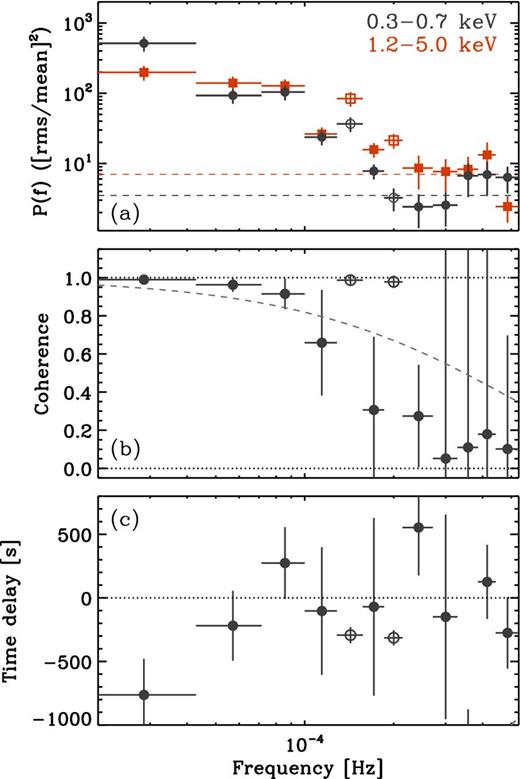
Cross-spectral products for the 0.3–0.7 and 1.2–5.0 keV bands. The data are binned as described in Section 4.1. Panel (a) shows the PSDs with Poisson noise level estimates from the best-fitting models described in Section 3. Panel (b) shows the Poisson-noise corrected coherence between the two bands. The dashed line is the function γ2(f) = exp (−f/5 × 10−4 Hz). Panel (c) shows the time delays, where a positive value indicates a hard band lag. The open symbols highlight the estimates at the QPO and harmonic frequencies.
From the cross-spectrum, we get the coherence γ2 (or squared coherency) between the two bands (e.g. Bendat & Piersol 1986). The coherence gives a measure of the linear correlation between the two bands, i.e. how much of one band can be predicted from the other. It is defined between [0,1], where 1 is perfectly coherent and 0 is perfectly incoherent. Fig. 5 panel (b) shows the coherence between the 0.3–0.7 and 1.2–5.0 keV bands. The coherence of the broad-band noise component is high (∼1) at low frequencies and decreases with increasing frequency. This pattern is typically observed in Seyferts (e.g. Alston et al. 2013). At the QPO and harmonic frequencies, we see ∼ unity coherence (open symbols), which sits above the falling broad-band noise coherence. Following Vaughan, Fabian & Nandra (2003a), we illustrate this by overlaying the function γ2(f) = exp (−f/5 × 10−4 Hz) in Fig. 5 panel (b). This describes the coherence of the broad-band noise fairly well, whilst the coherence at the QPO and harmonic frequencies are clearly distinct from this component.
From the cross-spectrum, we also obtain a phase lag estimate at each frequency, ϕ(f), which is transformed into the corresponding time lag τ(f) = ϕ(f)/(2πf), with errors estimated following (Bendat & Piersol 1986; Vaughan & Nowak 1997). We have previously performed extensive Monte Carlo simulations to check this method produces reliable error estimates when the contribution of Poisson noise is large (see Alston et al. 2013, 2014a). Fig. 5 panel (c) shows the frequency-dependent time lags between the 0.3–0.7 and 1.2–5.0 keV bands, where we follow the convention of using a positive time lag to indicate a hard band lag. A hard lag at low frequencies is typically seen in variable Seyferts (e.g. De Marco et al. 2013a). No significant hard lags in MS 2254.9−3712, but do see an ∼3σ negative (hereafter soft lag) at the lowest frequency. A highly significant (∼5σ) soft lag is also seen at the QPO and harmonic frequencies (open symbols).
We also measure the cross-spectral products between the 0.7–1.2 and 1.2–5.0 keV bands, but we do not show it here. The coherence between the two bands is ∼1 up to ∼3 × 10⁻⁴ Hz (i.e. above the harmonic frequency), above which the Poisson noise dominates. No significant lag is found at the QPO or harmonic frequency.
4.2 Time delays as a function of energy
A related technique is to study the time delays at a particular frequency as a function of energy. The lag-energy spectrum can be calculated by estimating the cross-spectrum between a comparison energy band versus a broad (in energy) reference band (e.g. Zoghbi et al. 2011; Alston et al. 2014a). If the comparison energy band falls within the reference band it is subtracted from the reference band, in order to have no correlated errors. We use the 0.3–5.0 keV band as the reference band due to its high S/N. We compute the lag-energy spectrum at a range of frequencies, including the broad-band noise (0.7–1.0 × 10⁻⁴ Hz), QPO (1.3–1.6 × 10⁻⁴ Hz) and harmonic and (1.8–2.1 × 10⁻⁴ Hz), and show these in Fig. 6. A positive lag value indicates the average band lag compared to the broad reference band.
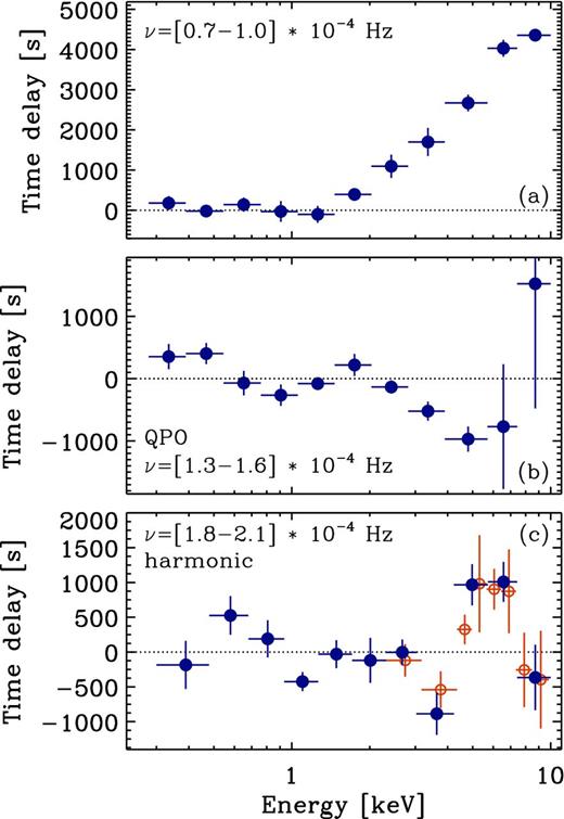
The lag-energy spectrum for the noise (0.7–1.0 × 10⁻⁴ Hz), QPO (1.3–1.6 × 10⁻⁴ Hz) and harmonic (1.8–2.1 × 10⁻⁴ Hz) frequencies. The open circles in panel (a) are the same data but with higher energy resolution.
The broad-band noise in panel (c) shows a lag that increases log-linearly between ∼1.0 and 10.0 keV. This trend is observed at low frequencies in BHBs (e.g. Miyamoto & Kitamoto 1989; Nowak et al. 1999a) and AGN (e.g. Papadakis, Nandra & Kazanas 2001; Vaughan et al. 2003b; McHardy et al. 2004; Arévalo et al. 2008; Kara et al. 2013c; Alston et al. 2014a; Lobban et al. 2014). The lag-energy spectrum shows zero lag between 0.3 and ∼1 keV.
The QPO lag-energy spectrum in Fig. 6 panel (b) shows, on average, the softer bands lagging behind the harder bands. This is consistent with soft lag seen between the lag-frequency spectrum in Fig. 5 panel (c). A similar lag-energy shape is observed at high frequencies in several Seyfert 1s (e.g. Kara et al. 2013c; Alston et al. 2014a). Many of these sources also display a lag between the primary continuum (e.g. 1.0–4.0 keV) and the iron Kα band at 6.4 keV. In the QPO lag-energy spectrum, the error bars are large above ∼5 keV and no clear lag in the iron Kα band is seen, hence we bin over from 5.0–10.0 keV. This is most likely due to the low number of cross-spectral estimates being averaged in this frequency band.
The lag-energy spectrum for the harmonic frequency is shown in Fig. 6 panel (c). A significant (≳4σ) lag is observed between the ∼1–4 keV continuum band and the ∼5–7 keV band, which contains the iron Kα band. To show the iron Kα lag is not sensitive to the choice of energy binning we compute the lag-energy spectrum at higher resolution (open symbols), which clearly follow the same shape. Despite the PSD being dominated by Poisson noise above 5 keV, we are able to pick out a significant lag at energies higher than this due to the significant power in the broad reference band and the high coherence between the energy bands.
The average lag between the 0.3–0.7 and 1.2–5.0 keV bands is soft, consistent with the lag-frequency spectrum at the harmonic frequency in Fig. 5 panel (c). A dip in the lag-energy spectrum at 3–4 keV compared to the remaining bands can also be seen at the harmonic in panel (c). This feature has now been observed in the high-frequency lag-energy spectra of several NLS1s (e.g. Kara et al. 2013a), but is yet to be explained.
4.3 Frequency-dependent energy spectrum
Using frequency-resolved rms-spectra, we investigate the energy dependence of the variability at different time-scales (e.g. Edelson et al. 2002; Markowitz, Edelson & Vaughan 2003; Vaughan et al. 2003b). We calculate the rms in a given energy band by integrating the noise subtracted PSD (using an rms normalization) over the frequency range of interest (i.e from 1/T to 1/2Δt). This gives the rms-spectrum in absolute units. The fractional rms-spectrum is obtained by dividing the rms-spectra by the mean count rate in each energy band. Following Poutanen, Zdziarski & Ibragimov (2008), we calculate errors using Poisson statistics. Energy bands are made sufficiently broad such that no time bins have zero counts.
We compute the rms-spectra in three frequency bands; 1.4–4.3 × 10⁻⁵ Hz (noise), 1.3–1.6 × 10⁻⁴ Hz (QPO) and 1.9–2.1 × 10⁻⁴ Hz (harmonic). Fig. 7 shows the rms-spectra in absolute units (panel a) and fractional units (panel b). The noise has a soft spectral shape, whereas the QPO and harmonic are both spectrally hard. This same dependence of spectral shape with frequency is observed in the NLS1 galaxies PG 1244+026 and RE J1034+396, which are also believed to be accreting close to the Eddington rate (Middleton et al. 2009; Middleton, Uttley & Done 2011; Jin et al. 2013).
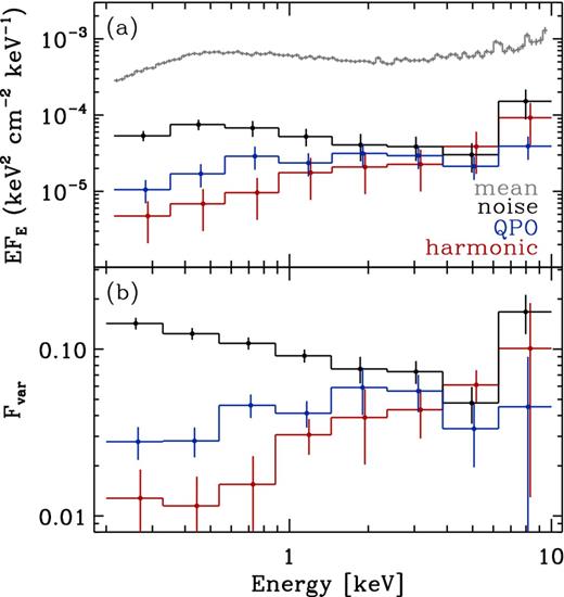
The frequency-resolved variability spectrum for the low-frequency noise (1.4–4.3 × 10⁻⁵ Hz), QPO (1.3–1.6 × 10⁻⁴ Hz) and harmonic (1.9–2.1 × 10⁻⁴ Hz) frequencies. Panel (a) shows the absolute rms-spectra as well as the mean (time-averaged) energy spectrum unfolded to a PL with index 0 and normalization 1 (i.e. ‘fluxed’ spectra). Panel (b) shows the fractional rms-spectrum (Fvar = rms/mean).
The time-averaged spectrum is also shown in Fig. 7 panel (a). We obtain a good fit to the data (χ2 = 773/784 degrees of freedom) with a spectral model consisting of two absorbed PL and a neutral reflection component pexmon (Nandra et al. 2007). The spectral index of the PL components are 2.84 ± 0.04 and 1.43 ± 0.06, respectively, consistent with the values reported in Bianchi et al. (2009). We use tbabs (Wilms, Allen & McCray 2000) for the total absorption and find a value of NH = 1.7 × 1020 cm−2, consistent with the value of neutral absorption from Willingale et al. (2013). The XMM–Newton RGS spectrum shows no signatures of ionized absorption. We fit the absolute rms-spectra at each frequency with a single absorbed PL, with NH fixed as above. The spectral index of the low-frequency noise is 2.7 ± 0.1, consistent with the soft component in the mean spectrum. The spectral index of the QPO and harmonic are 2.0 ± 0.1 and 1.5 ± 0.2, respectively. The spectral index of the harmonic is consistent with the hard PL required in the time-averaged spectrum. The smooth energy dependence of the QPO and harmonic variability suggests the QPO process is indeed present in the softer energy bands, despite the non-detection of the QPO in the PSD.
A related method for studying the variable energy spectra at a given time-scale is covariance spectra (Wilkinson & Uttley 2009). Using a high S/N reference band, the correlated variability is picked out in a given comparison band, thus improving the S/N of the variability spectrum compared to rms-spectrum. The covariance spectra can also be used to investigate the correlated variability between a given energy band and the remaining individual energy bands.
We compute the covariance spectra in the Fourier domain (Uttley et al. 2011, 2014; Cassatella, Uttley & Maccarone 2012) in the same frequency bands used for the rms-spectra. We use two reference energy bands to compute the covariance spectra; 0.3–0.7 and 1.2–5.0 keV. The covariance spectra from both reference bands are identical to the rms-spectra shown in Fig. 7. The same is true for any reference band investigated. This is unsurprising given the ∼ unity coherence observed between the soft and hard energy bands in Section 4.1.
4.4 Principle component analysis
A complementary way to investigate the spectral variability is PCA (e.g. Vaughan & Fabian 2004; Parker et al. 2014a). PCA decomposes a data set into a set of orthogonal eigenvectors, or principal components (PCs; Kendall 1975). When applied to X-ray data, the variability of the source spectrum is broken down into a set of variable spectral components. If the source variability consists of a linear sum of uncorrelated and spectrally distinct physical components then an exact description of the physical components is obtained. Whereas rms and covariance spectra are somewhat model dependent, in principle, PCA produces the individual variable spectral components in a model-independent way.
Fig. 8 shows the two PCA components. The majority of the variability is dominated by a component (PC1) that increases linearly with increasing energy band above ∼1 keV. The second component (PC2) accounts for ∼5 per cent of the variability and has a soft spectral shape. Fig. 8 also shows the first two PCA components for RE J1034+396 (from Parker et al. 2015). The primary PCA components are practically identical in shape and amplitude. The second PCA components both show a similar soft spectral dependence, however, RE J1034+396 is softer below ∼2.0 keV and is spectrally harder above ∼3 keV. Typical NLS1s (e.g. MCG–6–30–15; Parker et al. 2014a) have a PC1 which can be described by a soft PL (Parker et al. 2015). Their PC2 is due to spectral pivoting, and higher order PCs are associated with ionized reflection. The PCA of absorption-dominated Seyfert 1s also has a distinct spectral variability shape (e.g. NGC 1365; Parker et al. 2014b).

The first (top) and second (bottom) PCs for MS 2254.9−3712 and RE J1034+396. PC1 contains ∼90 per cent of the variability in each source and PC2 ∼5 per cent. The shapes of the PCs are remarkably similar in each source and are themselves different to the two primary PCs see in other Seyferts (Parker et al. 2015).
5 DISCUSSION AND CONCLUSIONS
We have presented an analysis of the energy-dependent variability in the Seyfert 1 galaxy MS 2254.9−3712, based on an ∼70 ks XMM–Newton observation. We found a significant (∼3.3σ) QPO at ∼1.5 × 10⁻⁴ Hz in the PSD of the 1.2–5.0 keV band. The QPO is coherent, Q ∼ 8, and has an rms of ∼6 per cent. No significant QPO is observed in softer energy bands, although there is evidence in the PSD for some structure at the QPO frequency.
A highly coherent soft lag is seen between the 1.2–5.0 and 0.3–0.7 keV bands at the QPO frequency and at the frequency ∼2 × 10⁻⁴ Hz. This strongly suggests the presence of a harmonic QPO component in a frequency ratio 3:2, although does not constitute a detection. The coherence of the broad-band noise is high at low frequencies and drops off at higher frequencies. The highly coherent soft lag suggests that the weak periodic feature seen in the 0.3–0.7 keV is actually the reprocessed hard QPO emission.
An iron Kα lag is seen at the harmonic frequency. If this frequency is indeed related to the QPO, then this is the first time this reverberation signature responding to a QPO modulation has been reported in the literature. An iron Kα reverberation lag responding to the QPO process was first observed in RE J1034+396 (Markevičiūtė et al., in preparation) making this feature unique to these two sources.
A soft lag is observed at the QPO frequency in MS 2254.9−3712 but the data are insufficient to detect a clear iron Kα lag at this frequency. If it is really absent at the QPO frequency, then the lack of an iron Kα reverberation lag suggests some geometrical dependence to the QPO and harmonic components: the disc can only respond to the harmonic oscillation, but not the QPO.
The variability of the QPO and harmonic has a hard energy dependence and are associated with the hard PL spectral component. No significant lag is observed between the 0.7–1.2 and 1.2–5.0 keV bands at any frequency. This could be due to the same spectral component, modulated by the QPO process at higher frequencies, dominating the spectrum across these energies. The X-ray and broad-band energy spectrum will be investigated in detail in a follow-up paper.
The similarities in the PCA of MS 2254.9−3712 and RE J1034+396 indicate the same variability process is occurring in these two sources. The primary PCA component in both sources has a hard spectral shape. The QPO is also preferentially detected at harder energies, indicating the QPO has an intrinsically hard spectral shape. Parker et al. measured the PCA in a sample of 26 objects and found the PCA of RE J1034+396 to be different to other well-studied Seyfert 1s. They performed extensive simulations to account for the wide range of spectral variability. However, the hard shape of the primary PCA component in RE J1034+396 could not be reproduced. This suggests the QPO variability is modulating the spectral components in a different way to the variability process dominating in other Seyfert 1s.
5.1 Comparison with previous results
GMV12 analysed the 0.2–2.0, 2.0–10.0 and 0.2–10.0 keV PSD of MS 2254.9−3712 and searched for the presence of QPOs. They reported no significant QPO in these energy bands. Our lack of significant detection in the 0.3–0.7 and 0.7–1.2 keV bands is consistent with their results. Our detection of a significant QPO in the 1.2–5.0 keV band is most likely due to the 5.0–10.0 keV being dominated by Poisson noise, thus affecting the detectability of the QPO over the broader energy band. Indeed, we repeated our analysis using the energy bands of GMV12 and find no significant QPOs.
GMV12 found very weak preference for Model 2. However, their best-fitting parameters were very unusual for this model (e.g. αhigh ∼ −8 for the 0.2–2.0 keV band). Our value of αhigh ∼ −4.5 is marginally consistent with the mean slope of ∼3.1 found for 15 sources with a strongly detected bend in GMV12. Our larger value could be indicating the presence of the QPO is distorting the continuum modelling. Our choice of higher quality data selection is most likely responsible for the different best-fitting model parameters found by GMV12.
5.2 Understanding the time delays
An approximately log-linear hard lag is observed at low frequencies (∼9 × 10⁻⁵ Hz) where the broad-band noise dominates. This is consistent with the observed time lags at low frequencies in BHBs and AGN, which are currently best explained by the model of radial propagation of random accretion rate fluctuations through a stratified corona (e.g. Arévalo & Uttley 2006). At the lowest frequencies investigated (∼3 × 10⁻⁵ Hz) a tentative soft lag is observed. This soft lag at very low frequencies has only been observed in a handful of Seyferts: the low-flux observations of NGC 4051 (Alston et al. 2013), MCG–6–30–15 (Kara et al. 2014) and NGC 1365 (Kara et al. 2015). The origin of this low-frequency soft lag is still unclear, and whether the same mechanism is responsible in the three sources it has been detected in so far.
Zoghbi & Fabian (2011) detected a soft lag at the QPO frequency in RE J1034+396, and found the soft lag to be broader in frequency than the QPO. We observe the QPO and soft lag in MS 2254.9−3712 to have the same frequency width (see Fig. 5). A14 found evidence for a QPO harmonic component in RE J1034+396. The broader lag observed in RE J1034+396 may then be due to the lag at the harmonic frequency, but the current data are insufficient to individually resolve this feature.
The time lags at the HFQPO frequencies in a sample of BHBs were presented by Méndez et al. (2013). With the exception of the 35 Hz QPO in GRS 1915+105, all of the lags detected were hard lags, different to what we observe in MS 2254.9−3712. The sign of the observed lag in accreting BHs could be due to the relative fluxes of the intrinsic and lagging components (e.g. the primary PL and soft reflection). Indeed, Alston et al. (2013) found a strong dependence on the lag direction with source flux in the NLS1 galaxy NGC 4051, with the flux changes dominated by changes in the primary continuum normalization (e.g. Vaughan et al. 2011). Alternatively, the sign of the observed lag may be due to some other system parameter, such as inclination. It is also possible that the hard lags observed by Méndez et al. (2013) are in fact the same lagging process seen above 10 keV in AGN with NuSTAR, which are inferred as the Compton hump lagging the primary continuum (Kara et al. 2014; Zoghbi et al. 2014).
5.3 QPO identification
In this section, we discuss the identification of the QPO in terms of LF or HF type. HFQPOs in BHBs typically have a fractional rms ∼5 per cent (Remillard & McClintock 2006). The 6 per cent QPO rms in MS 2254.9−3712 is consistent with the value observed in BHB HFQPOs, and the ∼8 per cent observed in RE J1034+396 (A14). A Q ≳ 2 is typically observed in HFQPOs in BHBs (e.g. Casella et al. 2004), consistent with our value of Q ∼ 8. HFQPOs in BHBs are observed to display harmonic components in their power spectra, with an integer ratio of 3:2 (e.g. Remillard et al. 2002, 2003; Remillard & McClintock 2006). We find strong evidence for the presence of a harmonic component with ratio 3:2, which strongly suggests this is an HFQPO in MS 2254.9−3712.
The QPO in MS 2254.9−3712 displays many similar timing properties to the HFQPO in RE J1034+396 (Middleton et al. 2011) and Swift J164449.3+573451 (Reis et al. 2012). The QPO in these two sources are also dominated by the hard X-ray component, suggesting a similar origin to the QPO in MS 2254.9−3712. The current best estimate of the mass of RE J1034+396 is |${M_{{\rm BH}}}\sim 1 {--}4 \times 10^{6}$| (Bian & Huang 2010). The factor ∼2 in QPO frequency observed in these two AGN is then consistent with the factor ∼2 in BH mass, if the QPO is caused by the same process which then scales linearly with BH mass.
HFQPOs are a common feature of the very high/intermediate state (steep PL state) in BHBs (e.g. Remillard & McClintock 2006). These states are also characterized by mass accretion rates at or near Eddington (e.g. Nowak 1995; van der Klis 1995). The BHB GRS 1915+105 displays HFQPOs at 35 and 67 Hz when in a super-Eddington state (e.g. Morgan, Remillard & Greiner 1997; Cui 1999; Belloni et al. 2006; Ueda, Yamaoka & Remillard 2009; Middleton & Done 2010). Wang (2003) has suggested that MS 2254.9−3712 is a super-Eddington accretor. RE J1034+396 (Middleton et al. 2011) and Swift J164449.3+573451 (Reis et al. 2012) are also believed to be accreting at or around Eddington. It is then natural to associate MS 2254.9−3712 to the high accretion rate states of BHBs, arguing in favour of an HFQPO in this source.
The HFQPO fundamental ν0 in BHBs approximately follows the relation of |$\nu _0 = 931({M_{{\rm BH}}}/{\,\mathrm{M}_{{\odot }}})^{-1}$| Hz, where ν0 is the unobserved QPO fundamental (Remillard & McClintock 2006). If the QPO we detect at ∼1.5 × 10⁻⁴ Hz is the harmonic 2ν0, then we estimate |${M_{{\rm BH}}}\sim 6 \times 10^{6} {\,\mathrm{M}_{{\odot}}}$|. This is consistent with the value |${M_{{\rm BH}}}\sim 4 \times 10^{6} {\,\mathrm{M}_{{\odot}}}$| determined from the RBLR–λLλ(5100 Å) relation (Grupe et al. 2004).
De Marco et al. (2013a) found a close relation between the soft lag frequency and BH mass in a sample of Seyfert 1s. Assuming the same reverberation process is occurring in MS 2254.9−3712, the frequency of the QPO soft lag would then indicate |${M_{{\rm BH}}}\sim 2 \times 10^7 {\,\mathrm{M}_{{\odot}}}$|. This is consistent with the higher BH mass estimate |${M_{{\rm BH}}}\sim 10^{7} {\,\mathrm{M}_{{\odot}}}$| (Shields et al. 2003), suggesting an HFQPO in MS 2254.9−3712. Alternatively, if the low-frequency soft lag is caused by the same reverberation process seen in De Marco et al. (2013a), a mass of |${M_{{\rm BH}}}\sim 10^8 {\,\mathrm{M}_{{\odot}}}$| is inferred, again consistent with an HFQPO.
LFQPOs have been observed up to ∼30 Hz in BHBs (Remillard & McClintock 2006). If the time-scale of this process scales linearly with BH mass, then we estimate an upper limit of |${M_{{\rm BH}}}< 1 \times 10^6 {\,\mathrm{M}_{{\odot}}}$|. Harmonic components to LFQPOs are often reported in BHBs; however, the frequencies are related by the ratio 2:1. The QPO in 2XMM J123103.2+110648 (Lin et al. 2013) is only detected below ∼2 keV and no evidence for a hard PL component is seen. The QPO rms in this source is ∼25–50 per cent, which is consistent with the rms of LFQPOs in BHBs. When LFQPOs are present in BHBs, the broad-band noise component has a flat shape, with α ∼ 1 (e.g. Remillard & McClintock 2006). This is inconsistent with the shape of the broad-band noise observed in MS 2254.9−3712, making it unlikely to be an LFQPO.
This source currently lacks a reverberation mapping mass estimate (e.g. Peterson 2004) which is required before the exact QPO mechanism can be robustly identified. From the arguments above, we propose the QPO observed in MS 2254.9−3712 is indeed the same as the HFQPO phenomenon observed in several BHBs. The origin of HFQPOs is still highly uncertain, but it is clear that it must be a physical process occurring in the direct vicinity of the BH. A long observation of MS 2254.9−3712 is required to independently confirm the presence of the QPO and harmonic component. If indeed the observed iron Kα reverberation is responding to the QPO process, this will allow us to understand both these processes in better detail, and provide an important constraint for any theoretical model for the origin of HFQPOs.
We thank the anonymous referee for constructive feedback that helped improve the manuscript. WNA, ACF and EK acknowledge support from the European Union Seventh Framework Programme (FP7/2013–2017) under grant agreement no. 312789, Strong Gravity. This paper is based on observations obtained with XMM–Newton, an ESA science mission with instruments and contributions directly funded by ESA Member States and the USA (NASA).
REFERENCES
APPENDIX A: PN AND MOS POWER SPECTRA
The PSDs of MS 2254.9−3712 presented in Section 3 are from the combined pn and MOS data. Here, we show the 1.2–5.0 keV band PSD for the individual instruments (pn; Fig. A1 and MOS 1+2; Fig. A2). The PSDs were computed as described in Section 3 using the 58 ks ‘clean’ light curves with Δt = 100 s.
The 1.2–5.0 keV band PSD and model fits to the pn data are shown in panel (a), for model 1 (red) and model 2 (blue). The data/model residuals for models 1 and 2 are shown in panels (b) and (c), respectively.
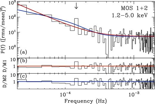
The 1.2–5.0 keV band PSD and model fits to the MOS data are shown in panel (a), for model 1 (red) and model 2 (blue). The data/model residuals for models 1 and 2 are shown in panels (b) and (c), respectively.
Both the pn and MOS 1.2–5.0 keV band PSDs display an outlier at ∼1.5 × 10⁻⁴ Hz. Model 1 is the preferred continuum model in both data, with pLRT = 0.002 and 0.024 for the pn and MOS, respectively. For Model 1, the pn only PSD gave pSSE = 0.004 and pR = 0.01, whereas the fit to the MOS PSD gave pSSE = 0.028 and pR = 0.006. Both these data indicate the presence of a significant outlier. Despite Model 1 being preferred, the p-values of Model 2 are moderately low, with pSSE = 0.01; pR = 0.04 for the pn, and pSSE = 0.033; pR = 0.005 for the MOS. This indicates the outlier at ∼1.5 × 10⁻⁴ Hz is also unusual under the best-fitting Model 2.
